ABSTRACT

Balancing agricultural needs with the need to protect biodiverse environments presents a challenge to forestry management. An imbalance in resource production and ecosystem regulation often leads to degradation or deforestation such as when excessive cultivation damages forest biodiversity. Lack of information on geospatial biodiversity may hamper forest ecosystems. In particular, this may be an issue in areas where there is a strong need to reassign land to food production. It is essential to identify and protect those parts of the forest that are key to its preservation. This paper presents a strategy for choosing suitable areas for agricultural management based on a geospatial variation of Shannon's vegetation diversity index (SHDI). This index offers a method for selecting areas with low levels of biodiversity and carbon stock accumulation ability, thereby reducing the negative environmental impact of converting forest land to agricultural use. The natural forest ecosystem of the controversial 1997 Ex-Mega Rice Project (EMRP) in Indonesia is used as an example. Results showed that the geospatial pattern of biodiversity can be accurately derived using kriging analysis and then effectively applied to the delineation of agricultural production areas using an ecological threshold of SHDI. A prediction model that integrates a number of species and families and average annual rainfall was developed by principal component regression (PCR) to obtain a geospatial distribution map of biodiversity. Species richness was found to be an appropriate indicator of SHDI and able to assist in the identification of areas for agricultural use and natural forest management.

Keywords:
species diversity; ecological impact values; forest planning and zoning; geospatial biodiversity mapping; principal component regression

Introduction

FAOSTAT (FAO, 2010Food and Agriculture Organization of the United Nations [FAO]. 2010. Global Forest Resources Assessment 2010. FAO, Rome, Italy. (FAO Forestry Paper, 163). Available at: http:// countrystat.org/home.aspx?c=FOR [Accessed Mar 20, 2013]
http://countrystat.org/home.aspx?c=FOR... ) indicated that forest conservation continues to be a significant ecological problem particularly in the tropical/subtropical forest biomes of South and Southeast Asia, Eastern and Southern Africa, and South America, and the temperate forest biome of Mongolia in East Asia. Agriculture is the most significant factor in worldwide deforestation (Kissinger et al., 2012Kissinger, G.; Herold, M.; De Sy, V. 2012. Drivers of Deforestation and Forest Degradation: A Synthesis Report for REDD+ Policymakers. Lexeme Consulting, Vancouver, Canada.). Unfortunately, deforestation for agricultural purposes is not always successful and can result in serious damage to the biodiversity of forest ecosystems while failing to achieve the proposed increase in agricultural production. A valid measurement of the biodiversity of forests is needed to build a framework for shaping public policies that steer or legislate economic activities towards maintaining overall biophysical sustainability (Smith, 1996Smith, F. 1996. Biological diversity, ecosystem stability and economic development. Ecological Economics 16: 191-203.). Such policies, particularly in under-developed countries are controversial as they require constraint of cropland expansion into forest areas, yet countries where this is an issue often see such expansion as key to regional/international food security (Krause et al., 2013Krause, M.; Lotze-Campen, H.; Popp, A.; Dietrich, J.P.; Bonsch, M. 2013. Conservation of undisturbed natural forests and economic impacts on agriculture. Land Use Policy 30: 344-354.). In order to address such subjects, many studies have focused on the reconciliation of conficts between land use changes and biodiversity (Wessels et al., 2003Wessels, K.J.; Reyers, B.; Jaarsveld, A.S. van; Rutherford, M.C. 2003. Identification of potential conflict areas between land transformation and biodiversity conservation in north-eastern South Africa. Agriculture, Ecosystems & Environment 95: 157-178.; Bawa et al., 2007Bawa, K.S.; Joseph, G.; Setty, S. 2007. Poverty, biodiversity and institutions in forest-agriculture ecotones in the Western Ghats and Eastern Himalaya ranges of India. Agriculture, Ecosystems & Environment 121: 287-295.; Henle et al., 2008Henle, K.; Alardb, D.; Clitherow, J.; Cobb, P.; Firbank, L.; Kull, T.; McCracken, D.; Moritz, R.F.A.; Niemelä, J.; Rebane, M.; Wascher, D.; Watt, A.; Young, J. 2008. Identifying and managing the conflicts between agriculture and biodiversity conservation in Europe: a review. Agriculture, Ecosystems & Environment 124: 60-71.; Prober and Smith, 2009Prober, S.M.; Smith, F. P. 2009. Enhancing biodiversity persistence in intensively used agricultural landscapes: a synthesis of 30 years of research in the Western Australian wheat belt. Agriculture, Ecosystems & Environment 132: 173-191.; Underwood, 2011Underwood, J.G. 2011. Combining landscape-level conservation planning and biodiversity offset programs: a case study. Environmental Management 47: 121-129.; Sandker et al., 2012Sandker, M.; Ruiz-Perez, M.; Campbell, B.M. 2012. Trade-offs between biodiversity conservation and economic development in five tropical forest landscapes. Environmental Management 50: 633-644.), combining efficient agricultural land use with biodiversity conservation. However the successful achievement of such a balance remains a significant challenge (Tscharntkea et al., 2012Tscharntkea, T.; Clougha, Y.; Wanger, T.C.; Jacksond, L.; Motzkea, I.; Perfectoe, I.; Vandermeer, J.; Whitbreadg, A. 2012. Global food security, biodiversity conservation and the future of agricultural intensification. Biological Conservation 151: 53-59.).

Recent research has proposed offsetting the costs of biodiversity protection and environmental services with an evaluation of the benefits to local people (Ferraro, 2001Ferraro, P. 2001. Global habitat protection: limitations of development interventions and a role for conservation performance payments. Conservation Biology 15: 990-1000.; Clements et al., 2013Clements, T.; Rainey, H.; An, D.; Rours, V.; Tan, S.; Thong, S.; Sutherland, W.J.; Milner-Gulland, E.J. 2013. An evaluation of the effectiveness of a direct payment for biodiversity conservation: the Bird Nest Protection Program in the Northern Plains of Cambodia. Biological Conservation 157: 50-59.), economic-based biodiversity value (Roy and Tomar, 2000Roy, P.S.; Tomar, S. 2000. Biodiversity characterization at landscape level using geospatial modelling technique. Biological Conservation 95: 95-109.) and ecological thresholds for biodiversity conservation (Huggett, 2005Huggett, A.J. 2005. The concept and utility of ecological thresholds in biodiversity conservation. Biological Conservation 124: 301-310.). Unfortunately, these methods are geospatially implicit, needing to be tailored to each particular environmental set of circumstances. Therefore, the aim of this study was to evaluate the feasibility of a strategy of differentiating areas in a forest ecosystem suitable for agricultural application and biodiversity conservation in the following sequence: (1) examination of the impact of the Indonesian Ex-Mega Rice Project on vegetational diversity; (2) development of a biodiversity prediction model, using principal component regression; and (3) identification of suitable zones for agricultural use and conservation management, using a moderate alpha diversity threshold.

Materials and Methods

Study site

The province of Central Kalimantan is located between 0°45′ N – 3°30′ S and 110°45′ E – 115°56′ E with altitudinal distribution up to 1800 meters above sea level (Figure 1). This province has about three million hectares of peatland, which is one of the largest unbroken tropical peatland areas in the world. The Indonesian Ex-Mega Rice Project (EMRP) was originally implemented by Indonesian Presidential Decisions (President Keputusan) No. 82,83/1995 in the 1990s to convert an area of around 146 million hectares of peat swamp forest into agriculture settlement, such as rice and palm-oil production (Aldhous, 2004Aldhous, P. 2004. Land remediation: Borneo is burning. Nature 432: 144-146.; Yassir et al., 2010Yassir, I.; Kamp, J. van der; Buurman, P. 2010. Secondary succession after fre in Imperata grassland of East Kalimantan, Indonesia. Agriculture, Ecosystems & Environment 137: 172-182.). Unfortunately, the EMRP led to unexpected consequences such as illegal forest exploitation, forest fire, air pollution, health hazards, lack of irrigation water and food shortage. As a result, the project was cancelled in 1999 (Aldhous, 2004Aldhous, P. 2004. Land remediation: Borneo is burning. Nature 432: 144-146.; Silvius and Diemont, 2007Silvius, M.; Diemont, H. 2007. Deforestation and degradation of peatlands. Peatlands International 2: 32-34.; Miettinen and Liew, 2010Miettinen, J.; Liew, S.C. 2010. Status of peatland degradation and development in Sumatra and Kalimantan. AMBIO 39: 394-401.; Blackham et al., 2014Blackham, G.V.; Webb, E.L.; Corlett, R.T. 2014. Natural regeneration in a degraded tropical peatland, Central Kalimantan, Indonesia: Implications for forest restoration. Forest Ecology and Management 324: 8-15.).

After the failure of the EMRP and following Presidential Instruction 2/2007 many efforts were made to restore numerous ecological, hydrological and biochemical functions and societal values of the peatland forest (Rieley and Page, 2005Rieley, J.O.; Page, S.E. 2005. Wise Use of Tropical Peatlands: Focus of Southeast Asia. ASEAN, Jakarta, Indonesia.; Rieley and Page, 2008Rieley, J.; Page, S. 2008. Master Plan for the Rehabilitation and Revitalisation of the Ex-Mega Rice Project Area in Central Kalimantan. A Joint Initiative of the Goverment of Indonesia and Netherlands. Euroconosult Mott McDonald, Arnhem, Netherlands.; Page et al., 2009Page, S.E.; Hoscilo, A.; Wösten, H.; Jauhiainen, J.; Silvius, M.; Rieley, J.; Ritzema, H.; Tansey, K.; Graham, L.; Vasander, H.; Suwido, L. 2009. Restoration ecology of lowland tropical peatlands in Southeast Asia: current knowledge and future research directions. Ecosystems 12: 888-905.; Miettinen and Liew, 2010Miettinen, J.; Liew, S.C. 2010. Status of peatland degradation and development in Sumatra and Kalimantan. AMBIO 39: 394-401.). Although the EMRP proved to be a notable failure, it still may be used as a typical example of how a geospatially explicit analysis could be used for zoning the suitable areas for agricultural use and biodiversity conservation.

The EMRP region in Central Kalimantan in 2009 was dominated by naturally healthy and partially degraded forests (38 %). The rest of the area consisted of severely degraded forests (14 %), shrub and grasslands (37 %), and agricultural land (including tree crops, 11 %) (Giesen and Meer, 2009Giesen, W.; Meer, P. van der. 2009. Guidelines for the Rehabilitation of Degraded Peat Swamp Forests in Central Kalimantan. Master Plan for the Conservation and Development of the Ex-Mega Rice Project Area in Central Kalimantan. Euroconsult Mott MacDermott, Jakarta, Indonesia.). The land in the EMRP region was divided into five blocks coded A-E. Only part of the blocks C and D, that are located respectively in the region ranging from 2°22′ S and 113°33′ E to 329′ S and 114°18′ E (Figure 1) and covering 440,000 ha and 139,000 ha, were used in this study. The inventory data was collected by Indonesia's National Forest Inventory (NFI) and offered by the Ministry of Forestry, Indonesia.

Field data system of Indonesia's National Forest Inventory

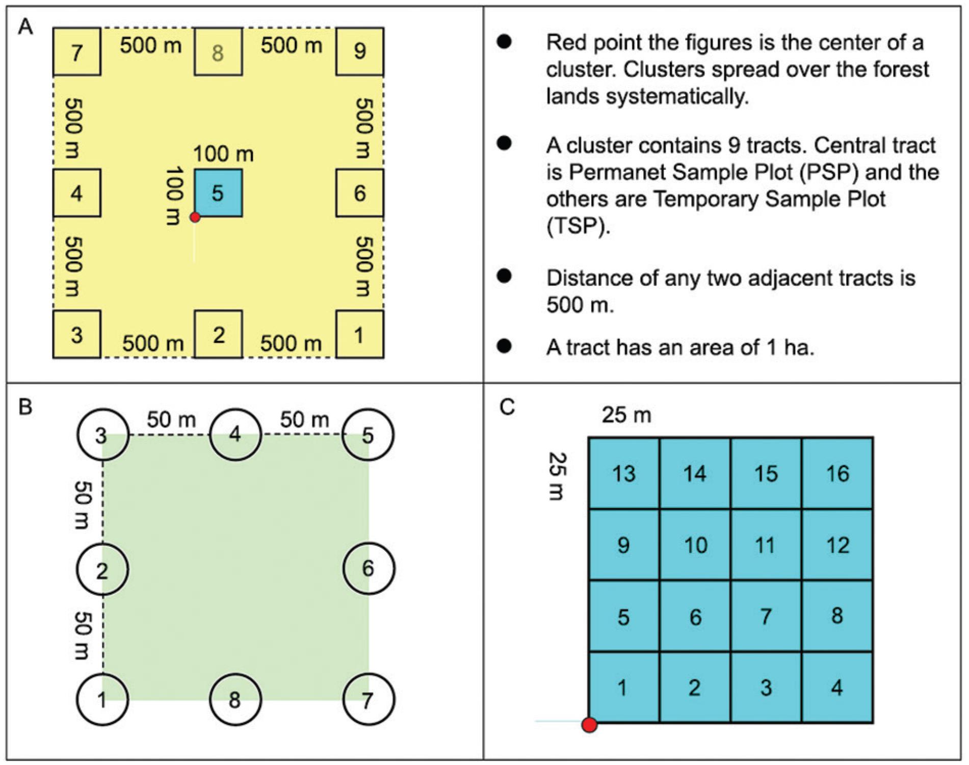
A multi-level systematic sampling method was applied in the NFI project to collect data for the estimation of timber volume, stand condition, species distribution, and species diversity. Firstly, the level one sampling unit was designated in terms of ‘clusters’. These were spread over the forest land systematically in a fixed spacing of 20 × 20 km. Secondly, a cluster was further divided into nine square tracts which were scattered spatially in a 3 × 3 matrix with the distance between the edge of any two adjacent tracts being 500 m (Figure 2A). The central tract was termed as the permanent sample plot (PSP) and the others as temporary sample plots (TSP). Thirdly, eight circle sub-plots were set on the boundary of the TSP for measurement using a point sampling technique (Figure 2B). Finally, the PSP tract was partitioned into 16 record units (RU) (Figure 2C). An inventory was conducted every 5 years. Data measured in the PSP were as follows: diameter of breast height (DBH), local name and name of the species and family. The NFI fieldwork was called Field Data System (FDS) by the Indonesia's Ministry of Forestry. The inventory data have been integrated with Geographical Information Systems (GIS) for use in forest resource management. The FDS data used in this study were from 1990 to 1996 and from 1996 to 2000 thereby representing the periods both before and after the EMRP. The data available for the analysis was from 15 PSPs and 240 RUs in the first period and from 2 PSPs and 32 RUs in the second period.

Explanatory variables and vegetational diversity

Data used for geospatial vegetational diversity mapping can be divided into two categories: biological and physical factors. Biological data in ecological studies are generally collected by forest inventory via ground plots. Based on the FDS data, several biological variables including species, family, frequency (number of individuals), and biomass were applied. The physical factors included meteorological variables such as rainfall, air humidity, monthly mean air temperature, and terrain variables such as elevation, aspect, slope, soil depth, and soil type. These physical variables are directly or indirectly able to influence the recruitment and growth of plants in forest ecosystems (Stanhill, 2011Stanhill, G. 2011. The role of water vapor and solar radiation in determining temperature changes and trends measured at Armagh, 1881-2000. Journal of Geophysical Research 116: D03105.). Meteorological variables were collected from the climate stations and terrain variables were also collected from the NFI project.

Shannon's diversity index (H'), abbreviated SHDI, is of major significance when considering regional vegetation biodiversity in this study. It estimates the uncertainty average in predicting which land cover type selected will be present in the habitat (Nagendra, 2002Nagendra, H. 2002. Opposite trends in response for the Shannon and Simpson indices of landscape diversity. Applied Geography 22: 175-186.). The formula for the determination of SHDI in a specific sample plot is:

where: S is the number of species, N denotes the total number of individuals, n_i stands for the number of individuals for a specific species i in a sample plot, p_i presents the proportion of each species in the samples, and ln is the natural log. The minimum value of SHDI is 0, while the maximum value is not infinite but limited to the combinations of the number of species and individuals at the site. SHDI = 0 indicates that the number of individuals are even equally distributed among all the species at the site.

Generation of geospatially continuous maps using the kriging interpolation method

Most of the biological and physical data were surveyed in geospatially discrete locations by sampling inventory. The observed data were used to determine the SHDI for the sampled plots. Fortunately, geospatial variables are generally highly autocorrelated in spatial arrangement (distance and direction) and thus can be used to predict unknown values from data observed at known locations. The process of prediction is known as geospatial interpolation. Ordinary kriging is one of the geostatistical techniques used for geospatial data interpolation/ optimal prediction (Journel and Huijbregts, 1981Journel, A.G.; Huijbregts, C.J. 1981. Mining Geostatistics. Academic Press, New York, NY, USA.; Isaaks and Srivastava, 1989Isaaks, E.H.; Srivastava, R.M. 1989. An Introduction to Applied Geostatistics. Oxford University Press, New York, NY, USA.; Cressie, 1990Cressie, N. 1990. The origins of kriging. Mathematical Geology 22: 239-252.).

Suppose a geospatial variable V(s) has been sampled at n locations (inventory plots) which spread over a forest landscape we are interested in. The symbol S_idenotes the location containing the spatial (x, y, z) coordinates. The general formula of ordinary kriging model is defined as:

where: V(S_i) is the measured value at the i^th location, w_ian unknown weight for the measured value at the i^thlocation, and

V(s₀) the predicted value for the un-sampled or prediction location S₀, andm is the number of samples which are distributed around that specific location. As shown in Figure 3, the m red-point samples (m ≤n) will be used to predict the value at the blue-point location. The weight, w_i, depends on a model fitted to the measured locations, the distance to the predicted location, and the spatial relationships among the measured values around the predicted location. Ordinary kriging uses a semivariogram to express the spatial variation, which minimizes any inherent error of predicted values that are estimated using spatial distribution (Jensen, 2005Jensen, J.R. 2005. Introductory Digital Image Processing: A Remote Sensing Perspectives. 3ed. Prentice Hall, Upper Saddle River, NJ, USA.). In this study, ordinary kriging is implemented on the SHDI, and also on biological and physical variables that are used for developing the vegetational diversity model.

Biodiversity modelling using principal component regression

An important criterion for selecting a forest area as a suitable candidate for conversion to agricultural use is that where a minimum impact on the nature of the greater forest environment should be the expected outcome. It is necessary to collect detailed vegetation information using intensive crew survey, for example as a minimum, the species and the number of each species in the forest community. Without such inventory data, it is impossible to derive biodiversity and to thus identify specific areas where biodiversity is significant. Therefore, a key purpose of this study is to examine if it is possible to apply environmental factors to the prediction of biodiversity.

Appropriate selection of environmental variables is critical for the performance of biodiversity models (Gillison and Liswanti, 2004Gillison, A.N.; Liswanti, N. 2004. Assessing biodiversity at landscape level in northern Thailand and Sumatra (Indonesia): the importance of environmental context. Agriculture, Ecosystems & Environment 104: 75-86.; Williams et al., 2012Williams, K.J.; Belbin, L.; Austin, M.P.; Stein, J.L.; Ferrier, S. 2012. Which environmental variables should I use in my biodiversity model? International Journal of Geographical Information Science 26: 2009-2047.). Environmental factors such as physical (elevation, slope, aspect, soil characteristics), meterological (temperature, humidity, rainfall) and land use are generally inter-correlated and also play important roles in biodiversity research. If two or more explanatory variables in a multiple regression model present a multicollinearity, the coefficient estimates may change erratically in response to small changes in the model or the data. An example is the cause-effect relationship between the dependent and independent variables being changed inversely. In this case, principal component regression (PCR) is appropriate in order to rule out multicollinearity by a linear combination of optimally weighted observed variables and uncorrelated effects (Jolliffe, 2002Jolliffe, I.T. 2002. Principal Component Analysis. 2ed. Springer, New York, NY, USA.).

PCR is a three-step procedure. In the initial step, principal component analysis (PCA) is applied to transform the possibly correlated kexplanatory variables into a set of linearly uncorrelated kprincipal components. The second step is to select fewer pcomponents which account for at least 80 % of the total variation in the original variables. Finally, an ordinary-least-squares multiple linear regression is carried out to generate a principal regression model,

where: β represents the regression coefficients for the firstp-components Z, and Y is the response variable. β₀stands for the intercept vector and ∊_i presents the error or residual of the estimate. Assessment of the biodiversity model was carried out by examining the deviation of the predicted results from the measured SHDI in the permanent sample plots.

Proposed strategy for the support of spatial decision-making

Briefly the strategy proposed is to implement an evaluation of the impact value of spatial diversity prior to management planning of natural forest ecosystem. Initially it is necessary to collect plot-based data by geo-spatial systematic sampling and ground inventory. Next, plot-based vegetational diversity such as SHDI and alpha diversity index are calculated. Thirdly the two-dimensional distribution map of vegetational diversity of the target forest is derived from kriging or principal component regression methods. Fourthly, a relatively low level of SHDI is suggested as the biodiversity threshold for differentiating areas. Finally, segmentation of the geo-spatial diversity map is implemented to partition agricultural and conservational management zones using the ecological threshold method. For example, if the SHDI of a specific area of land is less than the biodiversity threshold then the specific areas whose zoning code = 1 (the area could be developed) otherwise the zoning code = 0 (the area should be conserved). Thus it is not necessary to collect data for the entire forest area but as a result of our strategy, forest managers or planners will be able to easily identify areas of a forest that should be preserved, as they are significant with regards to biodiversity, and also to identify those areas that are less significant which may be considered for agricultural or other use. It should be noted that a determination of the ecological threshold method in the differentiation of land zoning could change based on a conservative strategy of sustainable forest management.

Results

Geospatial pattern of physical characters in the EMRP site

A significant reduction of the forested area was observed from 236,434 ha to 73,387 ha between the periods of 1990-1996 and 1996-2000, each of them representing a regular inventory span when data were collected and recoded in the FDS system. Inland parts of the areas are dominated by forests with greater soil depth, while the coast is dominated by non-forested areas that can be mangrove, bush/shrub, or swamp. The pattern of land use changes is shown inFigure 4A. Temperature and soil type are basically homogeneous around the study site. The site has an annual mean rainfall ranging from 1450 to 1515 mm and a soil depth between 50 and 1200 cm. The rainfall in the southern area is higher than in the northern area while the soil depth is thicker in the North-western area. The spatial distribution of average annual rainfall and soil depth is shown in Figures 4B and 4C.

Geospatial pattern of biological characters in the EMRP site

Investigation of biological factors in blocks C and D showed that the most abundant vegetation species were the belangiran (Shorea balangeran Burck) during the first period and jambu-jambu (Radermachera lobbii Miq) during the second period. From 1990 to 1996, 250 unique species of vegetation from a total of 35 different families were observed, with the most common (frequency/ number of individuals) being belangiran, malam-malam, meranti and galam. Some species are indicators of peat swamp forest, such as Ramin, Bintangur, Nyatoh, and Meranti, and the most dominant families were Dipterocarpaceae (13 %). The three greatest biomass species were ramin (Gonystylus bancanus Kurz) with 96 Mg ha^-1, tumih (Combretocarpus rotundatus Dans) with 65 Mg ha^-1, and bintangur (Calophyllum pulcherrimum) with 50 Mg ha^-1. The distribution of species by DBH and biomass in the two periods analysed changed dramatically from the periods before to those after the EMRP project (Figure 5). For example, average biomass was reduced from 113.07 to 39.19 Mg ha^-1 due to the project; and the number of species, families, and individuals before the EMRP was 288, 15, and 281 ha^-1 respectively, while these values dropped to 63, 6, and 63 ha^-1 respectively after the EMRP; and the average value of SHDI dropped from 2.58 to 1.45, which indicates a reduction in biodiversity.

In conjunction with the geospatial distribution pattern of the biological factors, Figures 6A, B, C, and D illustrate the kriged map of biomass, family richness (the number of families), species richness (the number of species), and frequency (the number of individuals) of the study, site respectively. A higher spatially heterogeneous pattern existed in the period before the EMRP project while this pattern became more homogeneous in the later period. For example, species richness (Figure 6C) was higher in the northern end of the region, which is covered by peat swamp forest, but later became higher in the southwest part of the region (in general with a smaller range than before), which is dominated by shrub/bush, and contains some dry land crops and secondary mangrove forests.

The geospatially continuous analysis of biological factors plays an important role in characterizing the impacts of reclamation activities in Kalimantan. These two types (original data and assumptions) made by kriging interpolation for other type of land use are shown in Table 1, where the difference found was not significant.

Discussion

Biodiversity impacted by EMRP and suggested implications

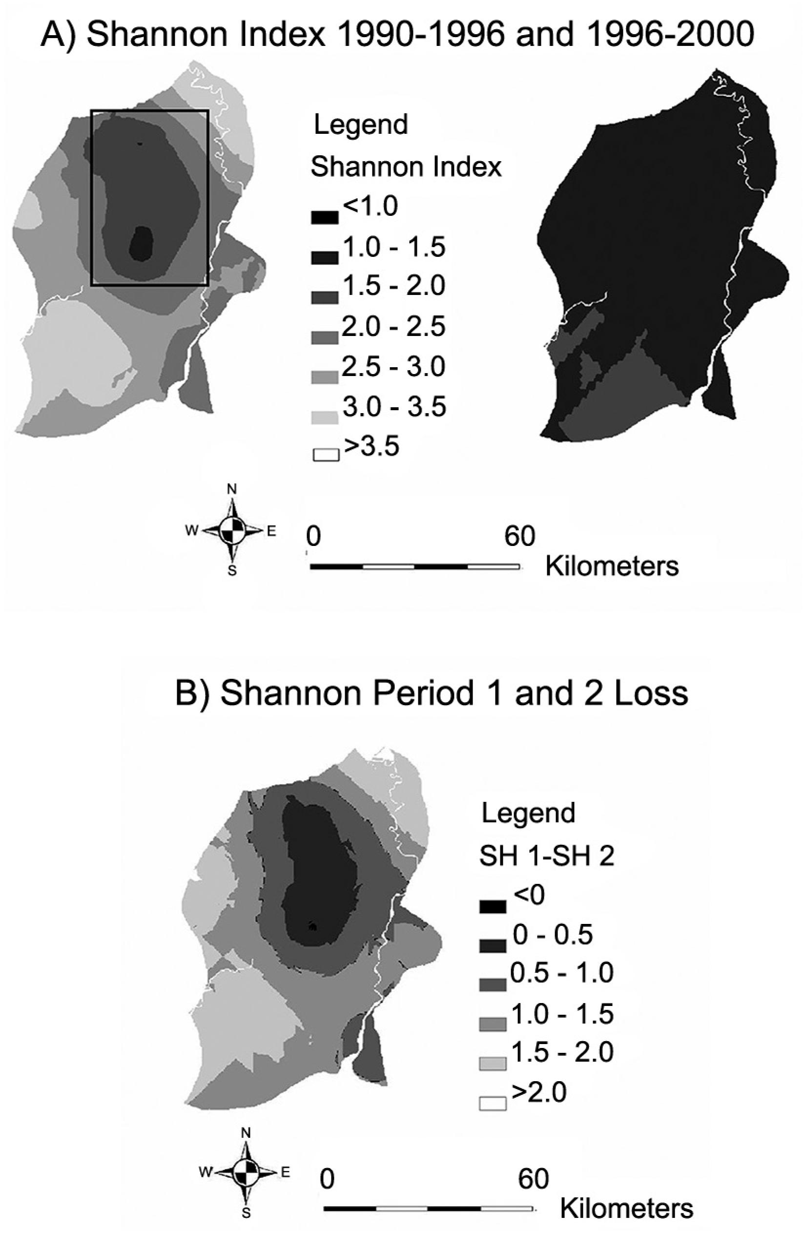
Kriging analysis showed that the distributions of the SHDI changed significantly from a range of 0.8-3.7 in 1990-1996 to 0.4-2.3 in 1996-2000. The average loss of SHDI was between −0.038 and −2.5 per hectare indicating a significant overall loss of biodiversity (Figure 7). The kriging estimation of SHDI yielded a minimum value similar to the diversity in upland areas, while the maximum values are comparable to those of peat secondary forests (Brearley et al., 2004Brearley, F.Q.; Prajadinata, S.; Kidd, P.S.; Proctor, J.; Suriantata, N. 2004. Structure and floristics of an old secondary rain forest in Central Kalimantan, Indonesia, and a comparison with adjacent primary forest. Forest Ecology and Management 195: 385-397.). This may have occurred due to natural disturbances of Indonesian forest prior to 1990; for example, El Niño caused some damage in 1986 and 1987, which though less severe than the disturbances in 1982-1983, 1997, and 2002 (Webster and Palmer, 1997Webster, P.J.; Palmer, T.N. 1997. The past and the future of El Niño. Nature 390: 562-564.), resulted in an increased number of forest fires and impacted the overall biodiversity in Indonesia (Murdiyarso and Lebel, 2006Murdiyarso, D.; Lebel, L. 2006. Local to global perspectives on forest and land fires in Southeast Asia. Mitigation and Adaptation Strategies for Global Change 12: 3-11.).

These projected SHDI maps can help identify the most suitable locations for rehabilitation, conservation, or even those with the best potential for agricultural purposes. For example, the box in Figure 7A shows an area with a smaller value of Shannon's diversity (SHDI < 2.0). In correspondence with Figure 6, this area also appears to have a lower level of species richness and biomass storage. An alternative approach for decision making purposes is, therefore, to consider this low-SHDI area as suitable for agricultural production while regions outside this area should be kept for environmental management, based on the conservation aim of ‘the minimization of the future loss of biodiversity’ defined by Witting and Loeschcke (1995)Witting, L.; Loeschcke, V. 1995. The optimization of biodiversity conservation. Biological Conservation 71: 205-207.. If conservation management had been successfully implemented in these high-SHDI areas, the amount of biomass storage that could have been maintained would have been more than 120 Mg ha^-1 since the 1990s. In other words, if the method proposed in this study could have been implemented prior to the determination of EMRP policy, it may have been possible to establish an appropriate zoning policy in the project areas with beneficial outcomes for both biodiversity and carbon management.

Evaluation of the biodiversity prediction model

As SHDI is determined by the number of species and the number of individuals of each species in the area, its determination would normally require intensive crew survey, which is very expensive. According to the correlation analysis, a significant agreement between biomass stock and the number of individuals and family richness and species richness, in particular SHDI-family richness-species richness, was observed. This underpins the PCR method as a key for estimating the SHDI of forests using these major biological and physical factors. Briefly, the number of species and families, and the average annual rainfall were deployed as variables for principal component analysis; then the first two components which accounted for 88 % of the total variance were used as regressors and the measured SHDI was used as a dependent variable in multiple linear regression analysis. The derived model for estimating Shannon's diversity is:

where: PC1 = 0.685X1 + 0.577X2 – 0.444X3 and PC2 = 0.041X1 + 0.578X2 - + 0.815X3; andX1 is the number of species, X2 represents the number of families, and X3 stands for average annual rainfall. This PCR-based model was evaluated with an R² of 0.77.

A new estimation of SHDI was made using the PCR-based model (Figure 8A) and evaluated using the SHDI map derived by the kriging method with the observed index values. The overall estimation bias was around −0.75 to 0.75 (Figure 8B). By comparing estimates with the observed SHDI, the PCR-based model was evaluated with prediction bias from 0.1 to 1.35 among the 15 FDS plots (Figure 9). A paired t-test was further conducted to examine the difference between the estimated and actual SHDI measured. It was concluded that there is no statistically significant difference (p < 0.05) between these two values.

Using vegetational alpha diversity as an indicator of SHDI for choosing suitable subsets of natural forest lands for agricultural uses

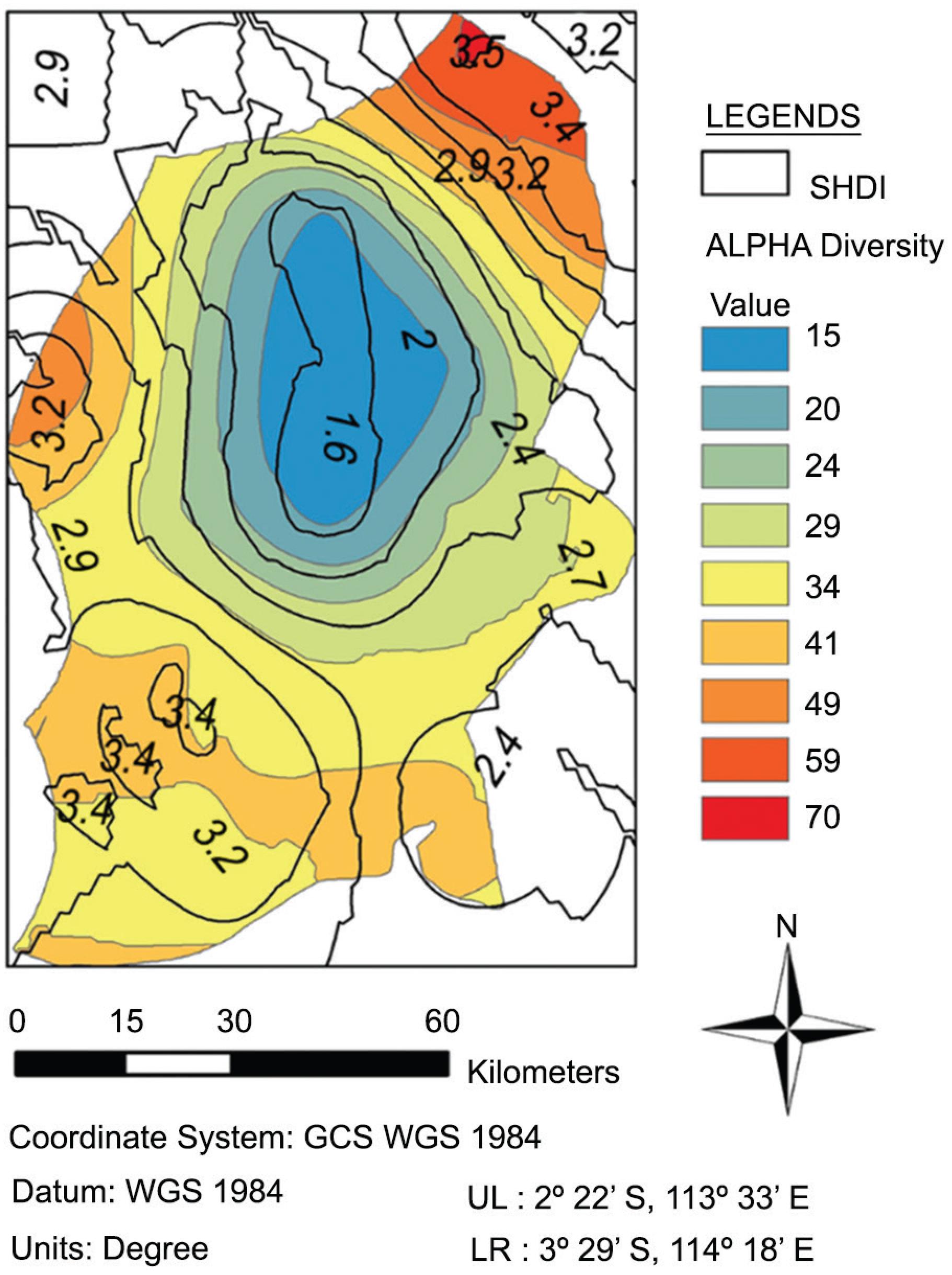
Alpha diversity refers to the number of species (i.e., species richness) within a particular area or ecosystem (Whittaker, 1972Whittaker, R.H. 1972. Evolution and measurement of species diversity. Taxon 21: 213-251.). As shown in Figure 10, the overlay of SHDI and alpha diversity in the study site demonstrates high spatial consistency between these two biodiversity indices. The lower value of SHDI (< 2.0) located at the central position of the site mostly overlaps with the lower value of alpha diversity (< 20) or completely covers the alpha diversity less or equal to 15. This suggests that vegetational alpha diversity could be used as an alternative index for choosing an area of relatively lower priority as regards biological conservation. This kind of relationship between landscape heterogeneity and plant species richness is similar to that seen on the Mexican Pacific coast (Priego-Santander et al., 2013Priego-Santander, Á.G.; Campos, M.; Bocco, G.; Ramírez-Sánchez, L.G. 2013. Relationship between landscape heterogeneity and plant species richness on the Mexican Pacific coast. Applied Geography 40: 171-178.).

If an alpha diversity of 20 is suggested as the ecological threshold for biodiversity conservation, the area suitable for agricultural use is almost equal to 18 % of the whole area of this study site; whereas if a more conservative threshold is suggested, such as an alpha diversity of 15, the developed area could be reduced to 10 %. As a result, around 82-90 % of the EMRP site area could be reserved for natural forest management.

Aspects other than biodiversity factors for balancing agricultural needs and conservation

The conversion of land to a variety of agricultural uses is a significant problem in the tropical, subtropical, and even temperate forest biomes (FAO, 2010Food and Agriculture Organization of the United Nations [FAO]. 2010. Global Forest Resources Assessment 2010. FAO, Rome, Italy. (FAO Forestry Paper, 163). Available at: http:// countrystat.org/home.aspx?c=FOR [Accessed Mar 20, 2013]
http://countrystat.org/home.aspx?c=FOR... ; Kissinger et al., 2012Kissinger, G.; Herold, M.; De Sy, V. 2012. Drivers of Deforestation and Forest Degradation: A Synthesis Report for REDD+ Policymakers. Lexeme Consulting, Vancouver, Canada.). In the case of national/regional inventories which involve both vegetation and wildlife geospatial data, the method proposed in this study is capable of deriving valuable geospatial information for governments to select appropriate areas for changes of use. Beyond the conservative development of forest ecosystem, fragmentation would be a concern as well as biodiversity and agriculture. Preventive maintenance of forest integrity or forest ecosystem connectivity should be a critical point to take into consideration before a determination of native land conversion is made. A piece of low-biodiversity forest should not be suggested as a potential site for agricultural development if the physical or soil properties do not show potential for reasonable agricultural productivity.

Conclusions

This study presented the strategy of applying forest inventory data to create geospatial distribution maps of SHDI and alpha vegetational diversities. Biodiversity heterogeneity of the studied site is, therefore, spatially explicit and can be used as a guide in the planning of forest management for achieving the goals of agricultural use, carbon storage, and biodiversity conservation/ functional biodiversity. Using a relatively lower level of the vegetational diversity (SHDI or alpha diversity) as a threshold criterion for forest development, a smaller subset of forest lands is suggested for agricultural use. This relatively low level of development should not lead to significant forest fragmentation, the resulting landscape combination somewhat resembling a large-scale natural habitat with moderate agricultural patches. As a result, a higher species richness of vegetational diversity and most of the natural forest ecosystem would be maintained sustainably. Alpha diversity can be used in a similar way to SHDI and can thus be directly used to simply derive the geospatial diversity of natural forest ecosystems for decision-making, and provide useful data for forest management and conservation.

References

Edited by

Publication Dates

History