Retrieval of Terrestrial Plant Fluorescence Based on the In-Filling of Far-Red Fraunhofer Lines Using SCIAMACHY Observations

1. Introduction

After chlorophyll molecules in plants absorb light, most of it is used for photosynthesis to convert carbon dioxide to sugars and molecular oxygen, O₂. A fraction of the energy absorbed, however, is re-emitted as fluorescence (Heldt, 2005). As a result of its relationship to photosynthetic efficiency, information on fluorescence can be used to assess the physiological state of the plant. In the last decades chlorophyll (Chla) fluorescence became an increasingly important non-invasive tool to investigate the efficiency of terrestrial or aquatic plant photosynthesis (Papageorgiou and Govindjee, 2004).

Triggered by the introduction of the Fraunhofer Line Discriminator method of Plascyk and Gabriel (1975) passive remote sensing of Chl fluorescence has been identified as a possibility to derive spatially resolved information. Even when the amount of Solar Induced Fluorescence (SIF) is small, it was shown (e.g., Moya et al., 2004; Corp et al., 2006; Campbell et al., 2008; Meroni et al., 2009; Rascher et al., 2009) that it provides valuable physiological information on terrestrial plants.

Chlorophyll fluorescence spectra typically span the spectral range from the red to the near-infrared with two pronounced peaks at around 690 and 740 nm. Within this wavelength range the additive signal emitted as SIF at canopy leaf or vegetation level alters the top of atmosphere (TOA) radiance. This additive signal leads to a proportionally larger fraction of the total upwelling radiance where the radiance is low (i.e., within telluric and solar Fraunhofer absorption lines). Recent investigations by Sanders and de Haan (2013) showed that this can also affect aerosol parameter retrievals in this wavelength range.

Several retrieval approaches have been published over the last few years to retrieve SIF from the data measured by passive remote sensing instruments operating in nadir viewing geometry. These methods use either strong absorption lines like the O₂-A band (e.g., Guanter et al., 2007) or selected stronger Fraunhofer lines like the Potassium (K I) line near 770 nm or the Ca II line near 866 nm (e.g., Joiner et al., 2011, 2012). Frankenberg et al. (2011a) could show that using solely the O₂-A wavelength region would not allow decoupling of spectral information of SIF from other contributing signals as a result of scattering by aerosols or clouds. Later, Frankenberg et al. (2011b), Joiner et al. (2012), Guanter et al. (2013), and Guanter et al. (2014) used a split-window approach (one on the left and one on right wing of the O₂-A band) utilizing more than just one Fraunhofer line to reduce the sensitivity of the retrieval to noise. Joiner et al. (2013) then developed a new approach utilizing a comparatively large window from 712 to 783 nm. However, as mentioned in Section 2.1 this spectral window is highly influenced by H₂O and O₂ absorption features related to the gaseous concentration and air pressure. Therefore, choosing a narrower wavelength range, free of gaseous absorption, could decrease the uncertainties due to these features.

A specific problem of the aforementioned retrieval approaches is the so called zero-offset effect, which has been first discussed by Frankenberg et al. (2011b). The zero-offset effect was defined as the amount of additive radiation not originating from SIF but other (instrumental) sources. It is noteworthy, that the term has been coined for Fourier Transform Spectrometers (FTS, such as GOSAT)- however, in the following we will use it also for grating spectrometers. As pointed out by Joiner et al. (2012, 2013) the instrumental signal non-linearity (GOSAT- Greenhouse gases Observing SATellite), straylight, calibration, dark current effects etc. (GOME-2—Global Ozone Monitoring Experiment II or SCIAMACHY—Scanning Imaging Absorption Spectrometer for Atmospheric CHartographY) can be sources of such additive radiation among other. The effect has been identified as a significant source of error in the retrievals. GOSAT based retrievals have been accompanied by an application of a zero-offset correction proposed by Frankenberg et al. (2011b) quantifying the size of the additive signal in absence of SIF as a function of the average radiance. Originally the authors (Frankenberg et al., 2011b) were considering retrievals over Antarctica or Sahara to quantify the effect due to a non-SIF additive component. Guanter et al. (2013) employed a similar approach but extended it to any vegetation-free region (not only to the above mentioned two) and Joiner et al. (2012) used cloudy pixels over ocean. Both, in Joiner et al. (2012) as well as in Joiner et al. (2013) SIF retrievals based on SCIAMACHY and GOME-2 measurements were implicitly corrected for the zero-offset effect using cloudy earthshine (radiance) reference spectra instead of solar irradiance. However, the result based on GOME-2 data (Joiner et al., 2013) were achieved with 25 spectral principal components from vegetation-free pixels of one day, which could compensate also for the zero-offset effects.

It was shown, that other sources of in-filling such as rotational or vibrational Raman scattering do not play an important role in the Near InfraRed (NIR; Vasilkov et al., 2013) and maximum values will hardly exceed 0.1% in-filling of the solar and telluric absorption lines.

Chlorophyll fluorescence is also used to assess the physiological state of phytoplankton (Falkowski and Kolber, 1995) and also in this field significant advances have been made recently (see for example Wolanin et al., 2015). However, within this study we confine ourselves to terrestrial plant fluorescence and focus on the presentation of:

(i) a new and independent approach for the SIF retrieval, which has generic character and can in principle be applied to all spectrometers measuring in the fluorescence emission wavelength range- even if the underlying feasibility study has been done so far only for SCIAMACHY;

(ii) the compensation of a zero-offset signal by a combination of techniques, which have been used by the above mentioned groups. The correction scheme, which allows also the use of narrow-wavelength-windows is applicable for data from all modern spectrometers. However, this work should be understood as a methods paper and one part of a series of studies detailing the newly developed SIF retrieval method and showing some aspects of its feasibility. Thus, the fact that the spatial resolution of the used SCIAMACHY data is rather low plays a secondary role owing the main goal of this paper. The authors think that this work can provide a new and rather independent view on this new topic which is beneficial as the already established algorithms so far have been published in absence of an independent quantitative quality assessment/validation.

In Section 2 the basic retrieval approach is described, based on a forward model and its inverse solution which are described in Sections 2.1 and 2.2. The model requires a net SIF spectrum at TOA, computed by a radiative transfer model, described in Section 2.3. The compensation of intervening spectral broadband effects is done similarly as in Differential Optical Absorption Spectroscopy (DOAS) using spectral polynomials and has been used before in bio-aquatic studies (such as Vountas et al., 2003, 2007). The used wavelength range is in the near-infrared, in the vicinity of one of the peaks of the emission spectrum of terrestrial plant fluorescence, in particular due to light emission of photo system I. The advantages of using this wavelength range are discussed in section Section 2.3 as well. As it is described in Section 2.4, we have used nadir measurements from the SCIAMACHY instrument aboard on ENVISAT, which provides a data record from the year 2002–2012. The zero-offset correction, which is necessary for the specific SIF retrievals shown in this paper is defined in Section 2.5.

The focus of Section 3 is on the retrieval results based on the method proposed in Section 2 and their comparison to SIF measurements by others: the retrieved SIF results at canopy level were compared and presented together with an updated version of the results from Joiner et al. (2013) in Section 3.2. Finally, conclusions and outlook are given in Section 4.

2. Retrieval Technique and Data

The solar induced fluorescence results in the emission of photons at the top of vegetation layer in the red and near infrared (NIR) spectral ranges. This additive spectral signal is superimposed on to diffuse radiation at canopy layer, resulting in a relative change of the reflected radiation at TOA. The main goal of the retrieval algorithm suggested below is to detect variations of the fluorescence signal using hyper-spectral satellite measurements of the backscattered solar radiation and to provide estimations of the fluorescence emission spectrum at the top of canopy layer.

As an input for the fluorescence retrieval algorithm will be used the Logarithm of Sun-normalized Radiance (LSR)

with I^m and $I_0^m$ being the measured radiance at TOA and extra-terrestrial solar irradiance, respectively, at the wavelength λ. The explicit notation of the dependence of S^m on other parameters such e.g., observation/illumination geometry, geographical coordinates of an instrument footprint, measurement time etc. will be omitted for the sake of clarity.

We remind the reader that the sun-normalized radiance is typically used for the solution of numerous inverse problems based on satellite-borne data because the division of the measured radiance by the solar irradiance leads to the significant decrease of the Fraunhofer line amplitude. The usage of the natural logarithm allows in turn to separate broadband spectral structure caused by the surface reflection and scattering processes in the atmosphere from high-oscillating remaining Fraunhofer structure caused by the filling-in of Fraunhofer lines due to trans-spectral processes or the so called zero-offset effect (Frankenberg et al., 2011b). We emphasize that exactly this remaining spectral structure is the main source of information used to derive the strength of fluorescence in the proposed retrieval technique.

2.1. Forward Model

To solve any inverse problem one needs to formulate the model of the measured quantity or so called forward model (Rodgers, 2000). In the case under consideration we introduce modeled LSR as follows:

where I⁺ is the simulated radiance at TOA influenced by SIF, I₀ is the extra-terrestrial solar irradiance (Kurucz, 1995), and ε_a is an additive signal not induced by SIF (zero-offset; Frankenberg et al., 2011b).

Multiplying the nominator and denominator under the logarithm in Equation (2) by the simulated radiance at TOA in absence of SIF, I⁻(λ), we have

Assuming that the additive component ε_a is significantly smaller than I⁺(λ), we obtain in a linear approximation the following expression for the forward model:

The second term in this expression is an important input for the fluorescence retrieval algorithm and will be called Fluorescence Reference (FR) spectrum, F:

The importance of this term becomes clear accounting for that the TOA radiance influenced by SIF is represented as follows:

where ${F}$_t(λ) is the fluorescence spectrum at TOA. Substituting Equation (6) into Equation (5) and restricting ourselves to an expansion of the logarithm into a Taylor series with linear term (with respect to ${F}$_t), we have

Accounting for that ${F}$_t is much smaller than I⁻, one can see from Equation (7) that the FR spectrum is directly proportional to the fluorescence spectrum at TOA. Moreover, it can be seen that the FR spectrum resembles the inverse solar spectrum and therefore links the strength of observable fluorescence with the amplitude of remaining Fraunhofer structure.

In order to formulate an inverse problem we assume that

• the variation of the fluorescence spectrum ${F}$_t(λ) at TOA can be quantified scaling the FR spectrum;

• the spectral shape of the unknown fluorescence spectrum at TOA, ${{F}}_t^{\prime }(\lambda )$, resembles the shape of an a priori one. Therefore, it can be estimated by scaling the a priori fluorescence emission spectrum, i.e.,

where ${{F}}_t^{\prime }(\lambda )$ is the unknown, and ${F}$_t(λ) the a priori fluorescence spectrum. Accordingly, f is the scaling factor;

• the same scaling factor f is used to estimate unknown fluorescence spectrum at top of canopy layer scaling the a priori one, i.e.,

where ${{F}}_b^{\prime }(\lambda )$ is the unknown and ${F}$_b(λ) is the a priori fluorescence spectrum at top of canopy layer (see Appendix, for details);

• the additive component ε_a(λ) will be approximated as spectrally constant (in the considered wavelength window).

Summing up, the forward model based on Equation (4) and the above mentioned assumption, for the measured radiance at TOA, influenced by unknown fluorescence emission, is adapted and formulated as follows:

The first term in this equation does not contains information about the strength of fluorescence emission but depends on unknown atmospheric and surface parameters such as atmospheric gaseous absorption, aerosol scattering and absorption, as well as surface reflection. Therefore, in order to mitigate the effects of gaseous absorption of unknown strengths as well as the spectral broadband effects of aerosol, molecular scattering and surface reflectance we will confine ourselves to a rather narrow wavelength range where practically no gaseous absorption can be observed. In particular, the suggested fluorescence retrieval algorithm utilizes measurements in the spectral window 748.5–753.0nm (see Section 2.3). Under this assumption the first term in Equation (10), owing to its spectral smoothness, can be approximated by a low order polynomial. Coefficients of the polynomial are fit parameters in the same manner as e.g., for ε_a. Therefore, for different absorption and scattering by aerosols, different polynomial coefficients will be obtained in the fitting process:

where a_i are polynomial coefficients and N is the degree of polynomial. From systematic computations using radiative transfer model we concluded that a third order polynomial can approximate all broadband features in the selected spectral window with sufficient accuracy. Moreover, the analysis of residuals after fitting of measured LSR does not demonstrate any remaining broadband spectral components. Please note that, although N = 3 is used for all polynomials, coefficients a_i vary in different minimization problems. Therefore, different polynomials are distinguished by their subscripts, namely m, C_a, and ε. Thus, the forward model is formulated as follows:

P_m(λ) refers to the third order polynomial fitted in Equation (12). It is noteworthy that our assumptions about scaling of a priori fluorescence spectrum (see Equation 9) and spectrally constant additive component ε_a are fully justified within such narrow spectral range.

2.2. Inverse Problem

The target parameters of the forward model given by Equation (12), i.e., f and ε_a can be obtained solving the following minimization problem:

where S′(λ) is substituted according to Equation (12). Unfortunately the minimization of quadratic form given by Equation (13) does not allow to estimate parameters f and ε_a simultaneously. This becomes obvious considering Equation (7) from which follows that F(λ) ~ 1∕I⁻(λ) ~ 1∕I⁺(λ) ~ 1∕I^m(λ) and, therefore, functions F(λ) and 1∕I⁺(λ) are strongly correlated.

To address this problem we define the linear relationship between F(λ) and 1∕I^m(λ) introducing a factor C_a which can be obtained through the solution of following minimization problem:

Using the obtained linear relationship, $1∕I^m(\lambda )\approx C_{a}F(\lambda )+P_{C_a}(\lambda )$, that was confirmed by numerous numerical simulations, it can be seen that $\epsilon ∕I^m(\lambda )=\epsilon C_{a}F+\epsilon P_{C_a}(\lambda )$. The term $\epsilon P_{C_a}(\lambda )$ is of course a polynomial as well. Consequently, the quadratic form given by Equation (13) can be rewritten as follows:

where the parameter to be retrieved is defined as

and P_ε(λ) compensates for $\epsilon P_{C_a}(\lambda )$ as well. It follows that the parameter ε represents the linear combination of additive component ε_a and fluorescence emission component ε_f = f∕C_a.

The estimation of the additive component ε_a can be achieved solving the minimization problem (Equation 15) for measurements over ground pixels free of SIF because f equals zero in this case. The retrieved results for ε_a for different ground pixels (see Section 2.5, for details) show the clear dependence of additive component on the measured radiance at TOA and can be approximated as

where a, b, and c are coefficients of the parabolic approximation, Ī_m is the measured radiance averaged over spectral window under consideration, i.e.,

λ₁ and λ₂ are the minimal and maximal wavelength of the spectral window used.

Having obtained the approximation of ε_a, the estimation of the scaling factor f is performed solving the minimization problem (Equation 15) for the measurements over ground pixels expected to be influenced by SIF. The retrieved parameter ε allows us in this case to determine the scaling factor f. Indeed, employing Equation (16) we have

where the additive component ε_a is calculated according to Equation (17) using the measured radiance I^m(λ).

The considered approach has been used throughout this study and involves in summary the following steps:

• Retrieval of additive component ε_a solving the minimization problem given by Equation (15) for measurements over ground pixels without impact of SIF.

• Quantification of ε_a, i.e., determination of parabolic approximation coefficients a, b, and c in Equation (17). Since also instrumental effects can contribute to ε_a which can vary faster than natural ones, coefficients of parabolic approximation were created on a daily basis.

• Determination of C_a solving the minimization problem given by Equation (14).

• Retrieval of the component ε solving the minimization problem given by Equation (15) for measurements over ground pixels influenced by SIF.

• Calculation of scaling factor f according to Equation (19) using estimated values of ε, ε_a, and C_a.

• The retrieval results are presented in the form of scaled spectrally averaged fluorescence emission at the top of canopy layer

It is worth to notice that the auxiliary variables C_a and ε could be excluded from the retrieval process. Indeed, the measurement over vegetated pixels can be used to estimate ε_a according to Equation (17) and the estimated value can be subtracted from the measured signal. Using this corrected LSR instead of S′(λ) on the left-hand side of Equation (12), one can see that the right-hand side is free of ${\epsilon }_a∕I^{-}(\lambda )$ and therefore, Equation (12) can be solved directly with respect to the parameter f without considering C_a and ε.

Although this would simplify the retrieval algorithm, our numerical experiments demonstrated that subtraction of the obtained ε_a from the measured radiance, leads to numerical instability of the fitting process. This can be explained by the fact that subtraction of the additive component ε_a decreases the remaining spectral structure of Fraunhofer lines and increases the impact of random errors, which is especially important in the case of the weak fluorescence signal. Taking into account this finding, in this investigation, we employed the retrieval algorithm which includes auxiliary variables C_a and ε.

2.3. Fluorescence Reference Spectra

The creation of a Fluorescence Reference spectrum according to Equation (5) necessitates a radiative transfer model. In this study we have used the well established and tested model SCIATRAN version 3.2 (Rozanov et al., 2014). SCIATRAN is a comprehensive radiative transfer code for the modeling of radiative processes in the terrestrial atmosphere and ocean in the spectral range from the ultraviolet to the thermal infrared including multiple scattering processes, polarization, thermal emission, and ocean-atmosphere coupling.

Throughout this study the scalar version of SCIATRAN has been used, ignoring thermal emission but accounting for multiple scattering processes and Lambertian surface reflection. TOA radiance I⁺ influenced by SIF was calculated using fluorescence emission spectrum ${F}$_b(λ) as a source term in the lower boundary condition of the radiative transfer equation (see Appendix, for details).

The spectral window to perform retrieval of the fluorescence emission and respectively calculate FR spectra has been selected according to the requirement formulated below:

• A sufficient fluorescence signal contribution is needed for accurate retrievals.

• The considered wavelength range is free of surface or telluric absorption features.

• The filling-in of Fraunhofer lines caused by the rotation and vibrational Raman scattering should be as minimal as possible.

Following these requirements, we selected a rather smaller spectral window between λ₁ = 748.5nm and λ₂ = 753.0nm. This window is free of gaseous absorption and located near the second (far-red) peak of fluorescence emission mainly generated by PS1. Although the selected window is ~5nm wide, it contains enough Fraunhofer lines (see Figure 1) which are the main source of information about the strength of fluorescence emission in the considered retrieval algorithm. Moreover numerical experiments show that rotational and vibrational Raman scattering does not play an important role in this spectral range Joiner et al. (2013) and maximum values will hardly exceed ~0.1% in-filling of the considered Fraunhofer lines.

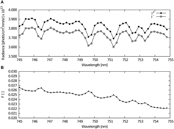
Figure 1. Example of basic radiance spectra used in this study. (A) Radiances I⁺ and I⁻ calculated with and without SIF contribution, respectively; (B) the FR spectrum F calculated according to Equation (5) and radiances shown in (A).

Another advantage of the selected window is that retrieved SIF in this window can be used to estimate Gross Primary Production (GPP). An approximate relationship between GPP and SIF is given e.g., by Frankenberg et al. (2011b), Guanter et al. (2013). The estimations of GPP and plant physiological state have been performed by Daumard et al. (2010) employing a narrow wavelength range nearby the O₂-A absorption band. However, such estimations are relatively complicated and their accuracy highly dependent on the vegetation functional properties and seasonal cycles.

In order to cover the full range of possible scenarios when using satellite-borne measurements we have calculated an ensemble of FR spectra (more than 170,000 scenarios) at high spectral resolution with varying observation/illumination geometries, surface reflectance and Aerosol Optical Depths (AOD). The selection of values and ranges has been done based on a sensitivity study utilizing extensive radiative transfer modeling (Khosravi, 2012). In particular the following values/ranges have been selected:

• viewing zenith angles including 0 and 10–40° on steps of 5°, 7 relative azimuth angles in the range 0–180° (for each 30°), and 7 solar zenith angles 0–40° (each 10°) as well as 60° and 80°;

• Lambertian surface reflectance values (focusing on typical values) in the utilized wavelength range at a step-width of 0.02 in the range 0.02–0.6 and a stepwidth of 0.05 in the range of 0.5–0.9 (in total: 40 values);

• AOD values at 750 nm in the range 0–1.5 (0.01, 0.02, 0.04, 0.08, 0.10, 0.20, 0.40, 0.60, 0.80, 1.00, 1.50).

The spectra were created for global observation conditions of all relevant spectrometers in orbit (or with available data) with needed spectral bands such as GOME, GOME-2, and SCIAMACHY.

The FR spectra were calculated by successive runs of SCIATRAN model at spectral resolution of 0.01 nm, convoluted to the required instrumental resolution using the appropriate instrument slit function, and saved in the form of global database. Gaussian slit function with full width at half maximum of 0.48nm was used in the case of the SCIAMACHY instrument. In order to mitigate impact of unknown in-flight slit function of SCIAMACHY (Burrows et al., 1999) the minimization of the quadratic form given by Equation (14) has been performed employing additionally shift and squeeze spectral correction parameters. Most adequate FR spectra are identified and (multidimensionally) interpolated to the actual satellite measurement conditions.

2.4. Application to SCIAMACHY Measurements

Initially we started this study using data from the satellite instrument SCIAMACHY (SCanning Imaging Absorption spectroMeter for Atmospheric CHartographY). SCIAMACHY is a grating spectrometer on board the ENVIromental SATellite (ENVISAT) (Burrows et al., 1995; Bovensmann et al., 1999). ENVISAT (with an equator crossing time of 10:00 a.m.) was launched in March 2002 to a sun-synchronous polar orbit and contact to this satellite was lost on 8th of April 2012. SCIAMACHY has spectral resolutions in different spectral channels ranging from 0.2 to 1.4 nm and has different spatial resolutions depending on the integration time. Its spectral band pass was divided into eight channels. The satellite instrument measured reflected, backscattered and transmitted solar radiation in four different observation modes: solar (and lunar) occultation mode as well as limb and nadir mode. For this study, nadir measurements from channel four have been utilized. The nominal spatial resolution of the instrument in nadir mode is 60 km across track by 30 km along track which was considered to be sufficient for this study. Unfortunately the selected wavelength range (748.5–753.0nm; see above) is given at lower spatial resolution (due to the increase of integration time), leading to ground pixel sizes of 240 km across by 30 km along track. Accordingly the spatial resolution of the retrievals (shown later) are useful whereever continuous vegetation prevails, such as the large tropical forests in South America and Africa. On the other hand, and as explained above, this study should be understood as a feasibility study specifying the abilities, requirements and limits of the presented method.

SCIAMACHY level 1b data have been used and all relevant corrections/calibration measures have been applied, among them radiometric calibration, straylight correction, correction for the memory effect, polarization and leakage current were the most important.

The global retrieval has been based on SCIAMACHY level 1 nadir data (Vers. 7.04).

2.5. Parameterization of Zero-Offset Effect

Retrieved values of the parameter ε obtained after solution of the minimization problem given by Equation (15) are presented in Figure 2. This figure shows individual retrievals of ε for one day of data as a function of the average radiance Ī_m (see Equation 18) using color codes. Only squares in green color show results retrieved over densely vegetated areas. All other colors and symbols show ε values for regions where SIF can safely be neglected. These results demonstrate that the filling-in of the considered Fraunhofer lines is observed not only in the case of pixels above vegetation but also for pixels above other surface types including cloudy conditions. This confirms that SCIAMACHY's radiance measurements contain an additive radiative component denoted above as ε_a (zero-offset effect).

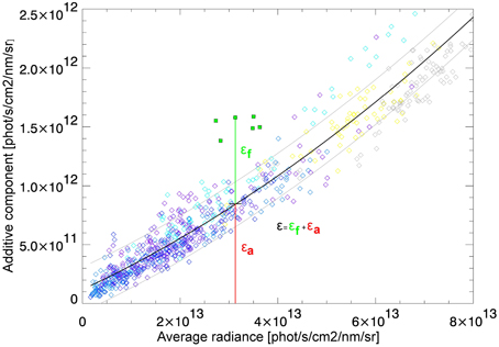
Figure 2. The additive component ε as a function of the average radiance Ī_m (see Equation 18): green symbols, in presence of vegetation; blue, over open ocean; gray, over permanent land ice; yellow, over desert; black solid line is the fitted curve; gray solid lines are ±σ standard deviation curves. All shown retrieval results in absence of vegetation might be affected by cloudiness.

In order to parameterize ε_a let us consider the retrieved ε values over regions free of vegetation. It follows from Figure 2 that they show a rather simple dependence on the measured average radiance and can be approximated by second order polynomial. The fitted curve (black line) along with ±σ standard deviation curves (gray lines) represent the parabolic approximation of retrievals over non-vegetated regions. It can be seen also that the retrieved values of ε over areas with vegetation appear to have a clear contrast and are well separated from the +σ deviation curve.

We consider the function given by Equation (17) as a good approximation in estimating the level of additive signal not induced by SIF but by other sources. Taking into account that according to Equation (19) the accuracy of the scaling factor f determination depends on the accuracy of approximation ε_a, we discuss below the selection technique of non-vegetated pixels which were used to create the most adequate estimations of ε_a.

2.5.1. Regions for Parameterization

In order to better separate the additive component caused by fluorescence, ε_f, from any other additive contribution, ε_a, whether natural or instrumental, we defined regions within which we do not expect any vegetation, thus no contribution by ε_f. For this purpose we selected pixels measured over areas such as oligotrophic open ocean water, desert sand and northern regions of Greenland or whole Antarctica. Additionally, as overcast or partly overcast regions exhibit a large span of brightness levels and a broad spatial extent such scenes were also incorporated in the creation of ε_a parameterization.

Potentially a part of the “natural” additive signal can arise over selected areas due to mineral luminescence from desert (Saharan) sand and rocks (Joiner et al., 2012) as well as due to chlorophyll-a fluorescence in the ocean water which has its peak contribution near 680nm. Although we do not expect significant contribution of chlorophyll-a fluorescence within selected oceanic regions shown in Figure 3 because of the strong liquid water absorption in the NIR spectral range and low concentration of Chl-a in such areas, we investigated the potential impact of chlorophyll-a fluorescence on the filling-in of Fraunhofer lines. Numerous calculations performed with coupled the ocean-atmosphere radiative transfer model SCIATRAN using different realistic assumptions about spectral width and position of this emission band did not show contribution of chlorophyll-a fluorescence within spectral window under consideration.

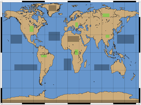
Figure 3. Gray boxes are considered to be non-influenced by plant fluorescence and are used for the determination of ε. Green boxes are expected to contain only ground pixels where ε is dominated by fluorescence. They are only used for demonstration purposes.

Thus, the measurements within gray boxes shown in Figure 3 were used to obtain parameterization of ε_a according to Equation (17). The coefficients a, b, and c of this parameterization were estimated on the daily basis (see next section).

2.5.2. Temporal Aggregation

To achieve a sufficient amount of retrievals to be able to fit a curve for ε_a the retrievals have to be aggregated temporally. One day of SCIAMACHY data led to around 1000 values of ε on average when considering the above defined areas. This allows stable fit results using a second order polynomial. Rarely (less then 20 times in 2008), very high values of ε (larger than 2·10¹³ phot s⁻¹cm⁻²nm⁻¹sr⁻¹) were obtained. We still have not identified the source for these very high values but exclude them in fitting for ε_a.

Figures 4A,B shows two daily examples (for March 1st and September 9th of 2008). The dependence between the average radiance and ε is shown through a corresponding quadratic fit specifying ε_a according to Equation (17). It can be seen that at moderate values of average radiances ε depends nearly linearly on it. The gray solid lines are ±σ standard deviation curves.

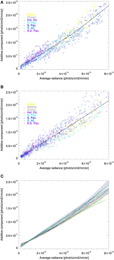
Figure 4. Dependence of the additive radiance component ε_a on the average radiance in the fit window, Ī_m, for one day of data for regions shown in Figure 3. (A) On September 9th, 2008; (B) On March 1st, 2008; (C) All fitted results for 2008- one line per day. The average slope (parameter b in Equation 17) is located at 0.02 and is well confined with ±0.01.

The scatter around the fitted curves increase for larger average radiances. The most important reason for this is the range of validity of the determination of ε and thus ε_a, because when deriving Equation (15) we restricted ourselves to a linear approximation. The lower panel of Figure 4 shows all fitted curves for 2008. Practically all of them are confined within a narrow band of the (gray) standard deviation curves of one of the example curves, such as in Figure 4 a for dark to moderately bright scenes (${Ī}_m<5·10^{13}$ phot s⁻¹cm⁻²nm⁻¹sr⁻¹).

This is giving rise to the assumption that we are confronted with a rather stable offset feature over 1 year and tests for other years confirmed a stable feature over several years.

From Figure 2 it becomes obvious that the retrieval quality of the scaling factor f is driven by the difference of ε and ε_a-values. For many data points this difference will not always be as pronounced. Certainly there are occasions where values of ε_f were above the fitted but below +σ curve. In order to assess how well values of ε_f are separated from ε_a (and corresponding +σ curve) on a global scale we binned all values ε (in absence of vegetation) and plotted the frequency of occurrence ε_f = ε − ε_a(Ī_m) for 1 year of data (2008) making up about 300,000 retrievals. The result is the gray colored distribution of ε_f in Figure 5. As expected the maximal number of occurrence corresponds to ε_f = 0.

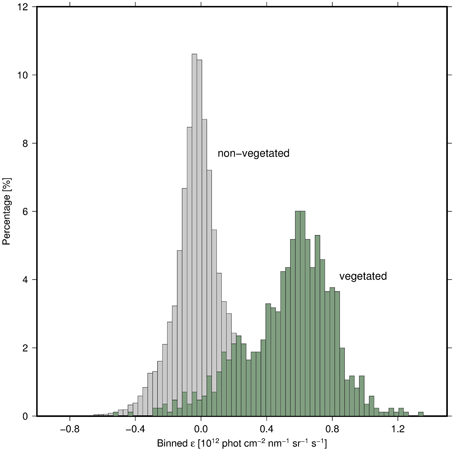
Figure 5. Distributions of ε_f = ε − ε_a(Ī_m) values for vegetated and non-vegetated regions shown by green and gray colors, respectively.

We repeated this exercise for expected fully vegetated regions (ε-retrievals over green-colored regions, Figure 3, for the year 2008 for about 10,000 retrievals). While the (gray) distribution for ε_f was centered around zero, the maximum value of the (green) distribution for ε_f is shifted to about 0.5·10¹² phot s⁻¹cm⁻²nm⁻¹sr⁻¹. In the zone were both distributions are well separated the estimation of f obtained according to Equation (19) is feasible. In the transition zone of both distributions the SIF retrieval is potentially hampered by other origins creating the additive component, such as for example instrumental effects.

3. SIF Retrieval Results and Comparison

As explained in Section 2.2 the SIF emission is retrieved according to Equation (20) in the form of spectrally averaged fluorescence emission spectrum, ${\bar{{F}}}_b^{\prime }$, and is used hereafter as a direct measure of the fluorescent emission strength (FES) expressed in [mW m⁻²sr⁻¹nm⁻¹] at the top of canopy layer.

In contrast to the retrieval of ε_a where the minimization problem given by Equation (15) can be solved using solely measured radiance and irradiance spectra, the retrieval of FES requires the proper selection of a FR spectrum to solve the minimization problem given by Equation (14), determination of a priori fluorescence emission spectrum ${F}$_b(λ) at the top of canopy layer, and auxiliary data to avoid cloud “contamination.”

To satisfy the first requirement the interpolation of FR spectra from the global database (see Section 2.3) was performed over the measurement geometry, surface reflectance, and AOD. Appropriate information about surface reflectance and AOD were obtained according to the database created from Koelemeijer et al. (2003) and given by Kinne et al. (2013), respectively.

The selection of a priori fluorescence emission spectrum has comparatively small impact on the result as stated by e.g., Guanter et al. (2013), Joiner et al. (2013). Studies using simulated data confirm also low sensitivity of the retrieved FES values with respect to variation of a priori fluorescence emission spectrum. Therefore, in the framework of this feasibility study ${F}$_b(λ) has been fixed to one emission spectrum and has been selected through FluorMODgui (Zarco-Tejada et al., 2006) for velvet grass (Holcus lanatus) as measured by Rascher et al. (2009). To properly describe the propagation of fluorescence emission through the atmosphere and interaction with aerosol particles and air molecules, the plant fluorescence radiative effect has been implemented into the SCIATRAN model by adding fluorescence emission spectrum as a source term in the lower boundary condition of the radiative transfer equation (see Appendix, for details).

Cloudy pixels or only partial overcast can have a significant impact on the retrieval of FES. The origin for this problem goes back to the estimation of ε_f (the additive radiative component induced only by SIF). As clouds can increase the brightness of the measured scene strongly, thus leading to an increased level of average radiance (see Figure 2) and ε_a is shifted to the rather unreliable part of the fitted parabola with stronger non-linear behavior and larger scatter of the data points. Therefore, the measurements contaminated by clouds were not involved in the retrieval process. For this purpose the MICROS (MerIs Cloud fRation fOr Sciamachy) cloud fraction data set (Schlundt et al., 2011) was used.

3.1. SIF Retrieval from Sciamachy Observations

Retrieval of FES has been performed for seasonally resolved averages of all available years (2003–2012), gridded to 80 arc minutes. Results were depicted in a color-coded fashion in Figure 6. The seasonal features for global distribution of FES are consistent with our expectation: Larger values of FES are observed over densely vegetated areas and a SIF “belt” is spanning from central Europe over Siberia to Eastern China during summer. This is also consistent with results shown recently in Guanter et al. (2013), Joiner et al. (2013), Guanter et al. (2014). An important aspect is the spatial resolution of our results. Originally each retrieval result is covering an area of 240 × 30km². Especially near the coasts the results are therefore likely to be influenced by water, leading to “diluted” values of FES because of lowered brightness and thus low values of ε_a and no contribution to ε_f by water. Accordingly, we retrieved rather low values of FES near the shores with consequences especially for the retrievals for example over the Indonesian Archipelago.

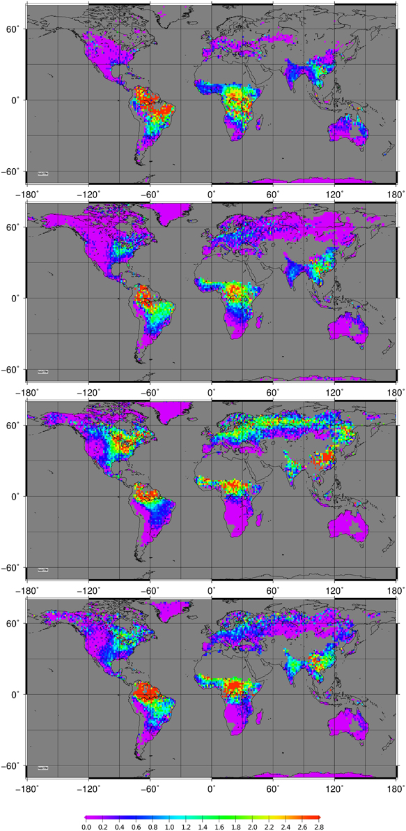
Figure 6. Global values of fluorescent emission strength in [mW m⁻²sr⁻¹nm⁻¹] at the top of canopy layer as seen from SCIAMACHY data. (1. upper) For Northern winter (DJF); (2. upper) For spring (MAM); (3. lower) For summer (JJA) and (bottom) For autumn (SON) months.

Larger variability which we expect over managed agricultural areas in Europe cannot be well resolved at this spatial resolution. The large and well pronounced US “corn-belt” is qualitatively in accordance with Guanter et al. (2014). They derived SIF-based crop GPP estimates which led to 50–75% larger results as from state-of-the-art carbon cycle models, especially in the US corn belt and the Indo-Gangetic Plain. The latter region is not as well pronounced in our results which might also be a consequence of the comparatively low spatial resolution used here and opposed to Guanter et al. (2014) were the spatial resolution of the GOME-2 based SIF retrievals was 80 × 40km².

3.2. Comparison with NASA Fluorescence Data

In this section we compare FES results obtained in the framework of this study with those reported by Joiner et al. (2014) which will be referred to NASA-data. Figure 7 depicts the resultant globally mapped data sets and scatter plot for the year 2009. In order to mitigate the difference in spatial resolution of SCIAMACHY and GOME-2 instruments, NASA-data (version 25) have been binned to the same grid as our retrieval results, namely to 80 arc minutes.

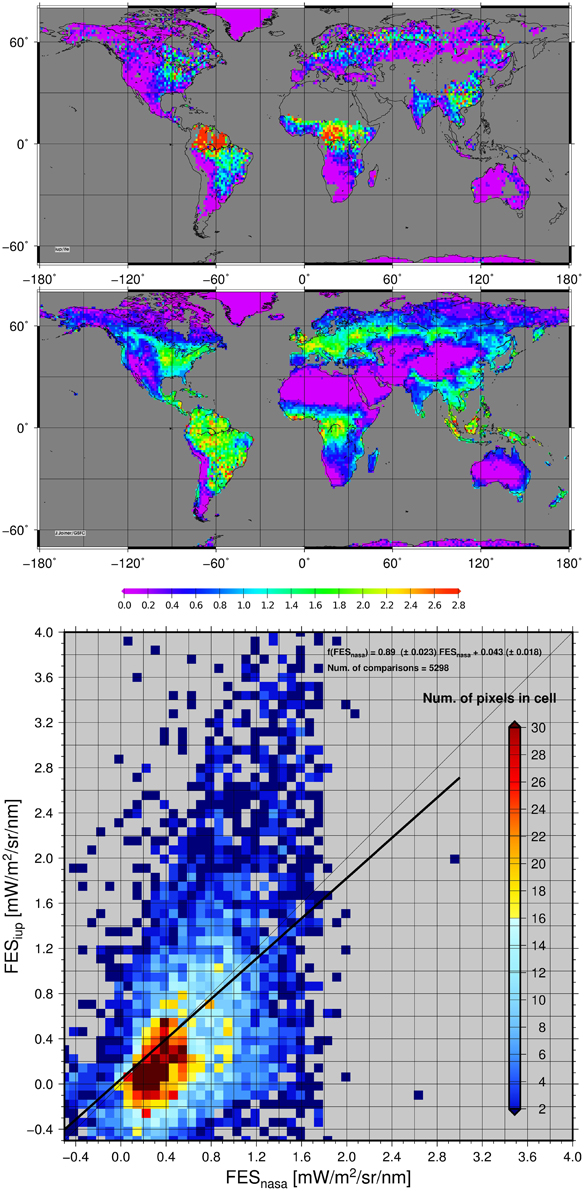
Figure 7. Global values of fluorescent emission strength in [mW m⁻²sr⁻¹nm⁻¹] at the top of canopy layer for the year 2009. Upper: results of this work, Middle: as reported in Joiner et al. (2013) (NASA), Bottom: a scatter (density) plot of both data sets with underlying color code (from dark red: frequent occurrence to dark blue: less occurrences).

Comparing results presented in the maps at upper and middle panels of Figure 7, one can state that typical hot-spots, such as the US-corn belt or the rain forests (and surroundings) are identified by both datasets. It can be seen also that the SCIAMACHY data set appears somewhat more patchy as compare to NASA-data. It can be explained due to the fact that SCIAMACHY achieves in its nadir-mode global coverage at the equator in 6 days whereas GOME-2 in ~1.5 days.

In addition we also performed a gridcell-by-gridcell comparison between the two data sets. The resulting scatter plot (Figure 7, bottom) depicts all gridcell comparisons. It can be seen that NASA values are confined within a narrow data interval with FES values less than ~2 mW m⁻²sr⁻¹nm⁻¹ while ours are ranging up to ~4 mW m⁻²sr⁻¹nm⁻¹. However, even if the scatter appears to be large, most of the values agree well in a range of FES less than ~1.5 mW m⁻²sr⁻¹nm⁻¹ and a linear regression line (black solid line in Figure 7, bottom) is close to the (gray) one-to-one line with regression slope of 0.890±0.023.

Although FES results obtained using SCIAMACHY measurements reproduce main features presented in NASA data set, we cannot expect to have identical results. The main reasons can be summarized as follows:

• In our case FES is averaged between 748.5 and 753.0nm whereas for NASA-data (version 25) the average FES between 734 and 758 nm is reported. The spectral interval used for averaging can lead to the different estimation of FES values. Comparisons with the previously published NASA-data sets (version 14) (Joiner et al., 2013) obtained using for averaging more wider spectral window confirms this suggestion. In particular, FES values of version 14 are larger than version 25 and showed closer agreement with our data especially over regions where our results tend to overestimate the current NASA-data (version 25).

• The low sampling of our retrieval results over certain areas especially over regions where persistent clouds obstruct the view to the canopy layer for longer time-spans. For Venezuela (Northern parts of South America) such conditions lead to gridded (averaged) values which were made up of 5 individual observations only, while in other less cloudy regions (and time spans) easily >30 individual observations were used for averaging 1 year of data.

• Some of the differences between two data sets are attributable to the different spatial resolution and local overpass time (Metop, the satellite carrying GOME-2, has an equator overpass time of 9:30 h, whereas that of ENVISAT carrying SCIAMACHY 30 min earlier).

Concluding we can state that the performed feasibility study confirms that the suggested retrieval algorithm of fluorescence emission strength can be successfully applied in combination with instruments having enhanced spatial resolution as compared to SCIAMACHY.

To the best of our knowledge, none of the recently published satellite-based fluorescence retrievals are quantitatively compared to independent measurements of known quality/accuracy (aka validation). Similarly, the comparison shown above cannot be understood as a validation and final judgment about the data quality needs further investigations.

4. Summary and Conclusions

A novel method for the retrieval of Solar Induced Fluorescence (SIF) has been developed. The method is using a micro-wavelength-window and is accompanied by a correction scheme which has been developed as part of this study to account for additive signals not originated by SIF. The application to 10 years of SCIAMACHY data showed promising results, where global SIF distribution is consistent with expected results and those already published by other authors. A direct comparison of our results with results from Joiner et al. (2014) based on Joiner et al. (2013) exhibited no clear picture. SIF values of our retrieval exhibit a broader value range [0–4 mW m⁻²sr⁻¹nm⁻¹], while Joiner et al.'s results were clearly confined within [0–2 mW m⁻²sr⁻¹nm⁻¹].

The approach presented here is of generic nature and can thus be applied to other data sets as well. We plan to apply the method to GOME-2 level 1 data, as the instrument has a better spatial resolution (in the wavelength range needed) and a better coverage, since this instrument is operated in nadir mode only, opposite to SCIAMACHY. This will also enable to have a direct (pixel-by-pixel) comparison with other authors using GOME-2, such as with Joiner et al. (2013) and Guanter et al. (2014).

Future effort will address the refinement of the input parameters of the retrieval and merge the SIF retrieval results with CO₂ absorption Buchwitz et al. (2005) retrievals to quantify CO₂ assimilation.

Conflict of Interest Statement

The authors declare that the research was conducted in the absence of any commercial or financial relationships that could be construed as a potential conflict of interest.

Acknowledgments

The funding of this work, coming from a DLR/BmWi grant, is gratefully acknowledged (FLUS, FKZ:50EE1260). The authors want to thank J. Joiner for the provision of data and S. Kinne for fruitful discussions.

References

Appendix

It is noteworthy that in the framework of this feasibility study we do not use any radiative transfer model to simulate fluorescence spectrum at the top of canopy (TOC) layer. Taking into account that the main goal of the proposed retrieval algorithm is to estimate the scaling factor of the a priori emission spectrum in the narrow spectral window, the fluorescence emission spectrum at the TOC layer, ${F}$_b(λ), has been selected through FluorMODgui (Zarco-Tejada et al., 2006) for velvet grass (Holcus lanatus) as measured by Rascher et al. (2009).

The terrestrial plant emission spectrum at TOC layer has a characteristic spectral shape such as shown in Figure A1 (for more details refer, for instance to Papageorgiou and Govindjee (2004). At top of atmosphere, however, this spectrum cannot be observed without the influence of gaseous absorbers, aerosol scattering and absorption, molecular scattering and surface reflection. Accordingly, the spectral radiance at TOA carries the spectral imprint of these various features. Among these processes fluorescence plays a comparatively small role, due to its low emission strength.

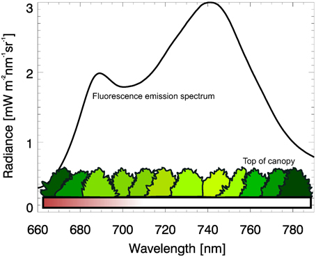
Figure A1. Fluorescence emission spectrum at the top of canopy layer in mW cm⁻²sr⁻¹nm⁻¹ (Rascher et al., 2009).

To properly describe fluorescence emission spectrum at TOA, we consider the propagation of fluorescence emission through the terrestrial atmosphere solving the following radiative transfer equation (RTE):

Details on how to derive this equation can be found among others in Chandrasekhar (1950); Hovenier et al. (2004); Pomraning (1991).

In Equation (21), I(τ, Ω) denotes the intensity of radiation field, τ∈[0, τ₀] is the optical depth changing from τ = 0 at TOA to τ = τ₀ at the bottom of the atmosphere, and the variable Ω: = {μ, φ} represents a pair of angle variables, μ∈[−1, 1] and φ∈[0, 2π]. Here, μ is the cosine of the polar angle ϑ measured from the positive z-axis and φ is the azimuthal angle measured from the positive x-axis in the clockwise direction when looking in the direction of the positive z-axis. The second term in the right-hand side is the scattering source function, where ω(τ) is the single scattering albedo (scattering coefficient divided by the extinction coefficient) and P(τ, Ω, Ω′) is the phase function describing the scattering properties of the medium.

The boundary conditions for RTE given by Equation (21) are formulated as follows: At the top of atmosphere, the incident solar radiation is assumed to be a monodirectional unpolarized light beam with an infinite extension in space. The solar zenith angle, ϑ₀, is defined as an angle between the positive direction of the z-axis and the direction to the Sun. The x-axis of the basic coordinate system is chosen to point away from the Sun. This means that the azimuthal angle of the solar beam is equal to zero (${\phi }_0=0^{°}$). The intensity of the direct solar light is written as I₀ δ(μ−μ₀) δ(φ−φ₀), where δ(μ−μ₀) and δ(φ−φ₀) are the Dirac delta functions Korn and Korn (1968), μ₀ is the cosine of the solar zenith angle, and I₀ is the extra-terrestrial solar irradiance. Throughout this study we have used I₀ according to Kurucz (1995). The upper boundary condition is formulated then as

At the lower boundary of the considered plane-parallel medium, we assume a Lambertian reflecting surface. The lower boundary condition is written then as follows:

where A is the Lambertian albedo, ${F}$_b is the fluorescence emission at TOC layer.

The solution of RTE obtained accounting for the formulated above boundary conditions is denoted as I⁺(τ, Ω). The simulated radiance in absence of SIF, I⁻(τ, Ω), is obtained solving the same RTE but setting in the lower boundary condition ${F}$_b = 0.

References

Bovensmann, H., Burrows, J. P., Buchwitz, M., Frerick, J., Noël, S., Rozanov, V. V., et al. (1999). SCIAMACHY: mission objectives and measurement modes. J. Atmos. Sci. 56, 127–149. doi: 10.1175/1520-0469(1999)056<0127:SMOAMM>2.0.CO;2
Buchwitz, M., Beek, R. D., Noël, S., Burrows, J., Bovensmann, H., Bremer, H., et al. (2005). Carbon monoxide, methane and carbon dioxide columns retrieved from SCIAMACHY by wfm-doas: year 2003 initial data set. Atmos. Chem. Phys. 5, 3313–3329. doi: 10.5194/acp-5-3313-2005
Burrows, J., Holzle, E., Goede, A., Visser, H., and Fricke, W. (1995). Sciamachy- scanning imaging absorption spectrometer for atmospheric chartography. Acta Astronaut. 35, 445–451. doi: 10.1016/0094-5765(94)00278-T
Burrows, J. P., Weber, M., Buchwitz, M., Rozanov, V., Enmayer, A. L.-W., Richter, A., et al. (1999). The global ozone monitoring experiment (GOME): mission concept and first scientific results. J. Atmos. Sci. 56, 151–175. doi: 10.1175/1520-0469(1999)056<0151:TGOMEG>2.0.CO;2
Campbell, P. K. E., Middleton, E. M., Corp, L. A., and Kim, M. S. (2008). Contribution of chlorophyll fluorescence to the apparent vegetation reflectance. Sci. Total Environ. 404, 433–439. doi: 10.1016/j.scitotenv.2007.11.004
Corp, L. A., Middleton, E. M., McMurtrey, J. E., Campbell, P. K. E., and Butcher, L. M. (2006). Fluorescence sensing techniques for vegetation assessment. Appl. Opt. 45, 1023–1033. doi: 10.1364/AO.45.001023
Daumard, F., Champagne, S., Fournier, A., Goulas, Y., Ounis, A., Hanocq, J.-F., et al. (2010). A field platform for continuous measurement of canopy fluorescence. Geosci. Remote Sens. IEEE Trans. 48, 3358–3368. doi: 10.1109/TGRS.2010.2046420
Falkowski, P., and Kolber, Z. (1995). Variations in chlorophyll fluorescence yields in phytoplankton in the world oceans. Aust. J. Plant Physiol. 22, 341–355. doi: 10.1071/PP9950341
Frankenberg, C., Butz, A., and Toon, G. C. (2011a). Disentangling chlorophyll fluorescence from atmospheric scattering effects in O2 a-band spectra of reflected sun-light. Geophys. Res. Lett. 38:L03801. doi: 10.1029/2010GL045896
Frankenberg, C., Fisher, J. B., Worden, J., Badgley, G., Saatchi, S. S., Lee, J.-E., et al. (2011b). New global observations of the terrestrial carbon cycle from gosat: patterns of plant fluorescence with gross primary productivity. Geophys. Res. Lett. 38:L17706. doi: 10.1029/2011gl048738
Guanter, L., Alonso, L., Gomez-Chova, L., Amoros-Lopez, J., Vila, J., and Moreno, J. (2007). Estimation of solar-induced vegetation fluorescence from space measurements. Geophys. Res. Lett. 34:L08401. doi: 10.1029/2007gl029289
Guanter, L., Rossini, M., Colombo, R., Meroni, M., Frankenberg, C., Lee, J.-E., et al. (2013). Using field spectroscopy to assess the potential of statistical approaches for the retrieval of sun-induced chlorophyll fluorescence from ground and space. Remote Sens. Environ. 133, 52–61. doi: 10.1016/j.rse.2013.01.017
Guanter, L., Zhang, Y., Jung, M., Joiner, J., Voigt, M., Berry, J. A., et al. (2014). Global and time-resolved monitoring of crop photosynthesis with chlorophyll fluorescence. Proc. Natl. Acad. Sci. U.S.A. 111, E1327–E1333. doi: 10.1073/pnas.1320008111
Hovenier, J. W., van der Mee, C., and Domke, H. (2004). Transfer of Polarized Light in Planetary Atmospheres. Basic Concepts and Practical Methods. Dordrecht; Boston, MA; London: Kluwer Academic Publishes.
Joiner, J., Guanter, L., Lindstrot, R., Voigt, M., Vasilkov, A. P., Middleton, E. M., et al. (2013). Global monitoring of terrestrial chlorophyll fluorescence from moderate-spectral-resolution near-infrared satellite measurements: methodology, simulations, and application to gome-2. Atmos. Meas. Tech. 6, 2803–2823. doi: 10.5194/amt-6-2803-2013
Joiner, J., Yoshida, Y., Vasilkov, A., Schaefer, K., Jung, M., Guanter, L., et al. (2014). The seasonal cycle of satellite chlorophyll fluorescence observations and its relationship to vegetation phenology and ecosystem atmosphere carbon exchange. Remote Sens. Environ. 152, 375–391. doi: 10.1016/j.rse.2014.06.022
Joiner, J., Yoshida, Y., Vasilkov, A. P., Middleton, E. M., Campbell, P. K. E., Yoshida, Y., et al. (2012). Filling-in of near-infrared solar lines by terrestrial fluorescence and other geophysical effects: simulations and space-based observations from SCIAMACHY and GOSAT. Atmos. Meas. Tech. 5, 809–829. doi: 10.5194/amt-5-809-2012
Joiner, J., Yoshida, Y., Vasilkov, A. P., Yoshida, Y., Corp, L. A., and Middleton, E. M. (2011). First observations of global and seasonal terrestrial chlorophyll fluorescence from space. Biogeosciences 8, 637–651. doi: 10.5194/bg-8-637-2011
Khosravi, N. (2012). Terrestrial Plant Fluorescence as Seen from Satellite Data. Master's thesis, University of Bremen, Inst. of Environmental Physics.
Kinne, S., O'Donnel, D., Stier, P., Kloster, S., Zhang, K., Schmidt, H., et al. (2013). Mac-v1: A new global aerosol climatology for climate studies. J. Adv. Model. Earth Syst. 5, 704–740. doi: 10.1002/jame.20035
Koelemeijer, R. B. A., de Haan, J. F., and Stammes, P. (2003). A database of spectral surface reflectivity in the range 335-772 nm derived from 5.5 years of gome observations. J. Geophys. Res. 108. doi: 10.1029/2002jd002429
Korn, G. A., and Korn, T. M. (1968). Mathematical Handbook for Scientists and Engineers. New York, NY; San Francisco, CA; Toronto, ON; London; Sydney, NSW: McGraw-Hill Book Company.
Kurucz, H. L. (1995). “The solar spectrum: atlases and line identifications,” in Laboratory and Astronomical High Resolution Spectra, ASP Conference Series, Vol. 81, eds A. J. Sauval, R. Blomme, and N. Grevesse (San Francisco, CA), 17–31.
Meroni, M., Rossini, M., Guanter, L., Alonso, L., Rascher, U., Colombo, R., et al. (2009). Remote sensing of solar-induced chlorophyll fluorescence: Review of methods and applications. Remote Sens. Environ. 113, 2037–2051. doi: 10.1016/j.rse.2009.05.003
Moya, I., Camenen, L., Evain, S., Goulas, Y., Cerovic, Z., Latouche, G., et al. (2004). A new instrument for passive remote sensing: 1. measurements of sunlight-induced chlorophyll fluorescence. Remote Sens. Environ. 91, 186–197. doi: 10.1016/j.rse.2004.02.012
Papageorgiou, C., and Govindjee. (2004). Chlorophyll a Fluorescence: A Signature of Photosynthesis. Dordrecht: Springer.
Plascyk, J. A., and Gabriel, F. C. (1975). The fraunhofer line discriminator mkii - an airborne instrument for precise and standardized ecological luminescence measurement. IEEE Trans. 24, 306–313. doi: 10.1109/tim.1975.4314448
Pomraning, G. C. (1991). Linear Kinetic Theory and Particle Transport in Stochastic Mixtures. Singapore; London: World Scientific Publishing.
Rascher, U., Agati, G., Alonso, L., Cecchi, G., Champagne, S., Colombo, R., et al. (2009). Cefles2: the remote sensing component to quantify photosynthetic efficiency from the leaf to the region by measuring sun-induced fluorescence in the oxygen absorption bands. Biogeosciences 6, 1181–1198. doi: 10.5194/bg-6-1181-2009
Rodgers, C. D. (2000). Inverse Methods for Atmospheric Sounding: Theory and Practice. Singapore: World Scientific.
Rozanov, V., Rozanov, A., Kokhanovsky, A., and Burrows, J. (2014). Radiative transfer through terrestrial atmosphere and ocean: software package SCIATRAN. J. Quant. Spectrosc. Radiat. Transf. 133, 13–71. doi: 10.1016/j.jqsrt.2013.07.004
Sanders, A. F. J., and de Haan, J. F. (2013). Retrieval of aerosol parameters from the oxygen a band in the presence of chlorophyll fluorescence. Atmos. Meas. Tech. 6, 2725–2740. doi: 10.5194/amt-6-2725-2013
Schlundt, C., Kokhanovsky, A. A., von Hoyningen-Huene, W., Dinter, T., Istomina, L., and Burrows, J. P. (2011). Synergetic cloud fraction determination for SCIAMACHY using MERIS. Atmos. Meas. Tech. 4, 319–337. doi: 10.5194/amt-4-319-2011
Vasilkov, A., Joiner, J., and Spurr, R. (2013). Note on rotational-raman scattering in the o2 a- and b-bands. Atmos. Meas. Tech. 6, 981–990. doi: 10.5194/amt-6-981-2013
Vountas, M., Dinter, T., Bracher, A., Burrows, J. P., and Sierk, B. (2007). Spectral studies of ocean water with space-borne sensor sciamachy using differential optical absorption spectroscopy (doas). Ocean Sci. 3, 429–440. doi: 10.5194/os-3-429-2007
Vountas, M., Richter, A., Wittrock, F., and Burrows, J. P. (2003). Inelastic scattering in ocean water and its impact on trace gas retrievals from satellite data. Atmos. Chem. Phys. 3, 1365–1375. doi: 10.5194/acp-3-1365-2003
Wolanin, A., Rozanov, V., Dinter, T., Nol, S., Vountas, M., Burrows, J., et al. (2015). Global retrieval of marine and terrestrial chlorophyll fluorescence at its red peak using hyperspectral top of atmosphere radiance measurements: feasibility study and first results. Remote Sen. Environ. 166, 243–261. doi: 10.1016/j.rse.2015.05.018
Zarco-Tejada, P., Miller, J., Pedrs, R., Verhoef, W., and Berger, M. (2006). Fluormodgui v3.0: a graphic user interface for the spectral simulation of leaf and canopy chlorophyll fluorescence. Comput. Geosci. 32, 577–591. doi: 10.1016/j.cageo.2005.08.010