Optical Classification of the Coastal Waters of the Northern Indian Ocean

1. Introduction

In an ocean under rapid modification by climate change, the boundaries between marine ecological provinces will move, but in ways that are difficult to predict (Karl et al., 1995; Platt and Sathyendranath, 1999). However, there is a premium on knowing the large-scale structure of the ocean ecosystem as it changes through time, in other words on developing and maintaining a biogeography of the ocean basin. Conventional biogeography relies on collecting and identifying individual specimens through samplings and survey techniques. At large geographical scales, it is a costly and time-consuming procedure to make even a single survey at one time point; making serial surveys to detect possible changes may be prohibitive on the grounds of expense. An alternative approach would be to use data streams from sensors carried on satellites in Earth orbit. Such data have the advantages of high-resolution at the ocean surface, high frequency of coverage, cost-effectiveness and synoptic coverage (Platt and Sathyendranath, 1999, 2008). Potentially, their use could yield a different kind of biogeography, based on data free from the limitations of coarse resolution in space and time. Visible spectral radiometry of the ocean provides a data stream that is particularly useful for ecosystem analysis: the visible spectrum carries information on the pigments and size of phytoplankton cells, as well as on the optical properties of the other constituents (such as suspended sediments and colored or chromophoric dissolved organic matter) in the surface waters of the ocean (Guzman et al., 1995; Babin et al., 2003; Dowell and Platt, 2009; Garaba and Zielinski, 2013). Mélin and Vantrepotte (2015) have pioneered the classification of coastal waters at global scale using annually-averaged fields of optical radiances from satellite data.

The Northern Indian Ocean is landlocked toward the north and bifurcates into two intra-continental seas: the Arabian Sea and the Bay of Bengal. Seasonally reversing monsoons and reversal of ocean currents are the major distinguishing features of the Indian Ocean basin (Shetye, 1998; Qasim, 1999). The monsoonal cycle, including southwest or summer monsoon and northeast or winter monsoon, determines the climate of the region. Southwest monsoon is the continuation of the southern hemisphere trade winds that bring monsoon rains and floods to the Asian landmass (Tomczak and Godfrey, 2001). Northeast monsoon is characterized by high pressure over the Asian land mass and northeasterly winds over the tropics and northern sub-tropics (Shetye and Shenoi, 1988). A strong coastal upwelling occurs along the western coast during the southwest monsoon season, whereas during the northeast monsoon season, cold continental winds cause convective mixing and winter cooling along the north Indian coast (Tomczak and Godfrey, 2001). Other oceanographic features of interest in this region include the Indian Ocean warm pool (Vinayachandran and Shetye, 1991) and monsoon depressions and cyclones (Schott and McCreary, 2001; Schott et al., 2009).

In the Northern Indian Ocean, biogeographical analysis has so far been restricted to what can be found using conventional methods (Krishnamurthy et al., 1978; Schills and Wilson, 2006; Obura, 2012, 2016; Jeffries et al., 2015). Few notable studies on global ocean biogeographic partitions using satellite datasets include: Longhurst province classification (Longhurst, 1998), based on regional oceanography of major oceanic basins, and a global database of chlorophyll profiles; and the 56 biogeochemical provinces proposed by Reygondeau et al. (2013) using the datasets of Sea Surface Temperature (SST), Chlorophyll and Sea Surface Salinity (SSS). The current study region includes at least parts of four provinces proposed by Longhurst (1998): the Red Sea and Persian gulf province (REDS), Northwest Arabian Sea upwelling province (ARAB), Western India coastal province (INDW), and Eastern India coastal province (INDE). Studies on biogeographic partitioning of the Indian Ocean region using remotely-sensed datasets are relatively few. Here, we follow the lead of Mélin and Vantrepotte (2015) through a detailed implementation of their optical remote-sensing method to the Indian Ocean region. We extend the temporal resolution to reveal seasonal changes in the optical classification of the coastal waters of the region. We interpret the results in the context of the seasonally-reversing wind and ocean current system that is the unique oceanographic characteristic of the region.

2. Data and Methods

2.1. Study Area

Northern Indian Ocean is subdivided by landmasses into the Arabian Sea in the west and the Bay of Bengal in the east and it opens into the equatorial Indian Ocean to the south. The Bay of Bengal coast is shared among India, Bangladesh, Myanmar, Sri Lanka, and the western part of Thailand. The Arabian Sea coast is shared among India, Yemen, Oman, Iran, Pakistan, Sri Lanka, Maldives, and Somalia. The area of interest is the coastal waters of the northern Indian Ocean within the 2,000 m isobath (Figure 1) (extending from 0 to 30° N latitude and 50 to 100° E longitude). Rather than using a more shallow depth (100–200 m) as the outer limit of the coastal zone, we have opted to use the 2,000 m isobath for the outer limit. This was to explore whether optical signatures of offshore waters appeared close to shore, and vice versa. In this choice, we were guided by Antony et al. (2002) who suggested that the offshore influence of coastal waters could extend as far out as 400 km from the shore. This region is well-known for the alternate upwelling and downwelling processes occurring during the contrasting seasons of southwest and northeast monsoons.

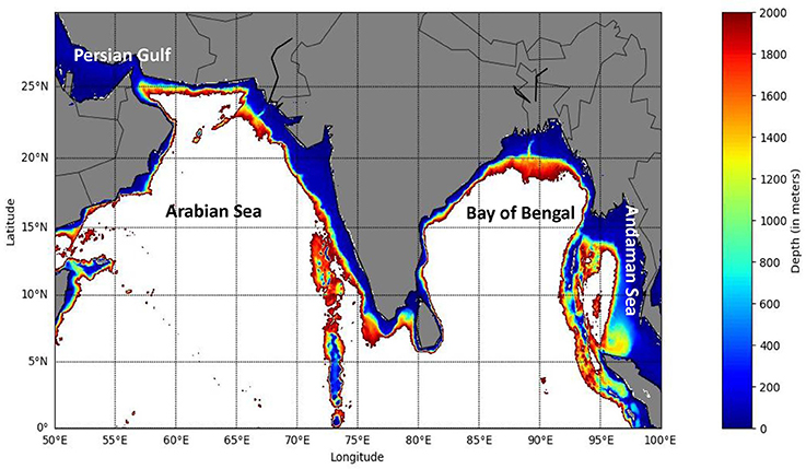
Figure 1. Northern Indian Ocean region showing 2,000 m and shallower isobaths.

Here, we use satellite remote-sensing reflectances (R_rs) at six wavelengths (412, 443, 490, 510, 555, and 670 nm) to identify optically-distinct regions of the coast. Figure S1 provides a schematic diagram of the methods used in the current study.

2.2. Satellite Dataset

Remote sensing reflectance (R_rs) of six wavelengths and Chlorophyll datasets were obtained from Version 2 of the Ocean Color Climate Change Initiative (OC-CCI, see www.oceancolour.org) (Sathyendranath et al., 2016, 2017) with spatial resolution of 4 km. Chlorophyll concentration was calculated from the remote-sensing reflectance, using the National Aeronautics and Space Administration (NASA) Ocean Color Chlorophyll Version 4 (OC4) algorithm (O'Reilly et al., 1998). This algorithm performed best in an algorithm comparison carried out as part of OC-CCI activities (Brewin et al., 2015). The OC-CCI satellite datasets affords superior coverage for the area of interest, compared with previously available data. These data products are band-shifted, bias-corrected and merged data archives obtained from three sensors: Sea-WIFS (Sea-Viewing Wide Field-of-View Sensor), MODIS-Aqua (Moderate Resolution Imaging Spectro-radiometer of the Aqua earth Observing System), and MERIS (Medium Resolution Imaging Spectrometer). OC-CCI datasets were validated using the in-situ datasets from Teledyne/Webb APEX-Argo floats deployed in the Arabian Sea (Roxy et al., 2016). The OC-CCI dataset are limited to the six SeaWiFS wavebands in the visible. We recognize the limitations of the bandset that were identified by Mélin and Vantrepotte (2015) for coastal optical classification. Therefore, the analyses and interpretation are restricted to the optical differences that are amenable to identification by the available dataset. All grid points of the selected region (depth range of 0–2,000 m) were used in the classification: grid points outside the 2,000 m depth range were excluded. Isobaths of the region were taken from the General Bathymetric Chart of the Oceans (GEBCO) 1-min gridded data set (Figure 1).

2.3. Normalization of Dataset

The remote-sensing reflectances (R_rs) at six wavelengths (412, 443, 490, 510, 555, and 670 nm) for the years 1998–2013 were used for the study. The remote-sensing reflectance values were skewed in their distribution and to minimize skewness, each R_rs spectrum was transformed to its log₁₀ values. They were then normalized by its integral from λ₁ (412 nm) to λ₂ (670 nm), where λ is the wavelength.

where $(\overrightarrow{x})$ (in units of nm⁻¹) indicates the normalized spectrum. The denominator was computed by trapezoidal integration. The normalization allows analysis of changes in the shape of the R_rs spectra, rather than in their magnitudes. Typically, changes in the shape of the spectra would be more affected by the composition of the materials present in the water, whereas the magnitude of the spectra is likely to be more indicative of the concentration of the substances, especially of highly-scattering substances. In this work, the vector ${\overrightarrow{x}}_j$ of six log-transformed and normalized reflectance values from a particular location and time (pixel, here indexed by subscript j) is referred to as an object. The total number of objects in a classification is N. Notation and Definitions used in this study are presented in Table 1.

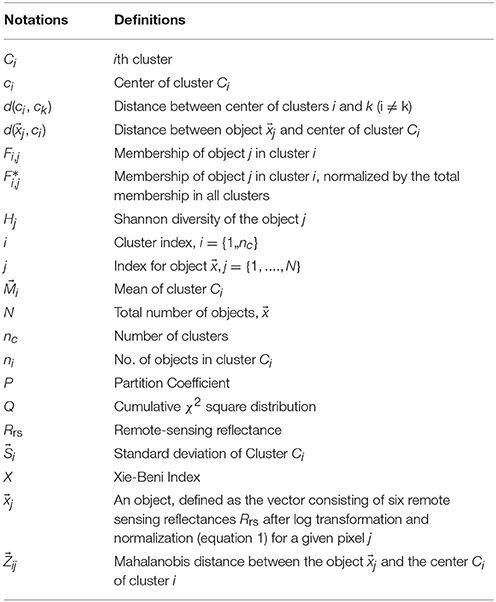
Table 1. Definition and Notations used in this study.

2.4. Fuzzy C Mean Algorithm

Fuzzy classification evolved from classical set theory. The classical clustering approach determines whether an object is a member or non-member of a given set of any system. Only these two options are possible. In contrast, fuzzy logic allows that an object may have partial memberships in more than one set. The classification algorithms based on fuzzy logic are often used in classifying data from natural systems. The method allows for overlap between boundaries of particular classes or sets, and recognizes that more than one class may be represented at a particular location at any given time.

The membership F_ij of a cluster i in the object j is given by $(1-Q({\overrightarrow{Z}}_{ij}^2))$ where ${\overrightarrow{Z}}_{ij}$ is the Mahalanobis distance given by $({\overrightarrow{x}}_j-{\overrightarrow{M}}_i)/{\overrightarrow{S}}_i$ where ${\overrightarrow{M}}_i$ is the mean, ${\overrightarrow{S}}_i$ is the standard deviation and Q is a cumulative χ² distribution (Zadeh, 1965).

In this study, the log-transformed, normalized reflectance spectra $(\overrightarrow{x})$ were analyzed using the Fuzzy C-mean (FCM) algorithm. Our implementation of fuzzy C mean classification follows Moore et al. (2001). It calculates the centres of each class or cluster and the percentage membership of each class in the data at each pixel. The FCM algorithm also uses several validity functions to assess the optimal number of clusters to be chosen for the classification (Bezdek, 1973; Rezaee, 2010).

2.5. Optimal Cluster Validity Functions

Cluster validity function is a statistical measure used to select the optimal number of clusters in the classification (too many clusters would imply that individual clusters resemble each other; too few would imply that all possible cases are not covered). We have used two methods: 1. Xie-beni index and 2. Partition co-efficient. These two methods are used only for selecting the optimal cluster number to run the fuzzy C-means classification. Cluster validity methods are statistical functions that determine the performance of a clustering procedure. Criteria of merit for a clustering method include the distance between clusters (separation) and the distribution of points around a cluster (compactness) (Deborah et al., 2010). We can rely on multiple validity functions to aid selection of the optimal cluster number. The principal strategy used is to cluster the data over a range of cluster numbers (n_c) and evaluate each clustering result with each validity function (Moore et al., 2009).

The Partition Coefficient and the Xie-Beni index are cluster validity methods designed specifically for use with fuzzy algorithms. These two methods are preferred to aid selection of the optimal number of clusters in fuzzy classification (Halkidi et al., 2001).

2.6. Xie-Beni Index

The Xie-Beni index X is one of the measures used to determine the best cluster number for the fuzzy classification of a particular dataset. This index depends on the geometric properties of the dataset and the membership matrix. To calculate X, we need to calculate two quantities: the sum over all clusters of the mean squared distance of each data object from the centre c_i of cluster C_i; and the square of the minimum distance between two cluster centers (Xie and Beni, 1991). The ratio of these two quantities is the Xie-Beni index:

The smallest value of the index indicates the best cluster number (Halkidi et al., 2001; Zhao et al., 2009).

2.7. Partition Coefficient

The Partition Coefficient P is a validity function that uses the membership values (F_ij) to provide the optimal cluster number. It measures the amount of overlap between clusters. It is defined as the ratio of the sum of squares of the membership matrix elements of all the clusters to the total number of objects.

The index values lie in the range [1/n_c, 1], where n_c is the number of clusters. The closer the value is to one the better the data are classified. The cluster number with a maximum partition coefficient is said to be the best cluster number to choose for classification (Bezdek, 1973; Bezdek et al., 1984).

2.8. Optical Diversity

Optical diversity is an indicator of the overall variability in optical constituents at a given space and time. Optical diversity, (H_j) is defined here, following Mélin and Vantrepotte (2015), by analogy with the Shannon Diversity Index (Shannon, 2001),

where $F_{i,j}^{*}$ is the normalized membership of the optical classes and n_c is the number of classes represented. The membership F_i,j was normalized by the integral of F_i,j over all optical classes to obtain $F_{i,j}^{*}$ :

3. Results and Discussion

3.1. Selection of the Optimal Class Number

The Xie-Beni Index and the Partition Coefficient were calculated for monthly climatologies of $\overrightarrow{x}$ for the study area, computed from the OC-CCI monthly R_rs climatologies, which are based on years 1998–2013. Monthly values allowed study of seasonal variations in the distribution of optical classes in this region, which is known for its pronounced seasonality. Climatologies were selected to minimize the effect of outliers through averaging, and also to improve the coverage and reduce gaps in data. Climatological data also provide a baseline against which trends in anomalies can be studied at a future date. Both indices varied between months, and the Xie-Beni index often showed a broad minimum, whereas the Partition Coefficient often showed a broad maximum, such that selection of the optical class number was not straightforward. Nevertheless, eight emerged as the optimal number. To aid the selection of optimal class number further, we also studied the maps of cumulative membership (sum of the memberships of all the classes) calculated using class numbers n_c from 5 to 15. The maps were studied for evidence of over-classification (large areas where the cumulative membership was >1) and under-classification (large areas where cumulative membership was <1). This study also showed that n_c = 8 gave the best compromise, with low numbers of both under-classified and over-classified pixels. Therefore, finally, eight classes were selected as the optimal cluster number for all the analyses presented here.

3.2. Identification of the Optical Classes

The mean spectra ${\overrightarrow{M}}_j$ of the eight selected optical classes are shown in Figure 2. Optical class 1 is characterized by a maximum in the blue, with the signal decreasing progressively toward the red, indicative of clear oceanic waters. With increasing class number, the signal decreased steadily at the shortest wavelength (412 nm), and the maximum shifted toward longer wavelengths: the maximum is at 490 nm for class 6 and 555 nm for class 8. Conversely, class 1 has the minimum value in the red at 670 nm, whereas classes 7 and 8 have the highest values in the red. The values of the mean spectra at the six SeaWiFs wavelengths for each of the classes and their corresponding covariance matrix are provided in Tables S1, S2. It is useful to assess how these optical classes relate to Case-1 and Case-2 waters as defined by Morel and Prieur (1977) and Prieur and Sathyendranath (1981). From the shapes of the spectra, it appears that classes 1–6 are representative of Case-1 waters and classes 6–8 of turbid Case-2 waters.

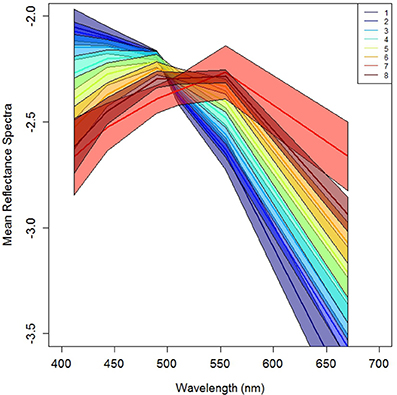
Figure 2. Mean Reflectance Spectra ${\overrightarrow{M}}_i$ of the eight optical classes, with the envelopes corresponding to the Mean ± SD.

The distributions of the dominant classes of representative months of the four seasons are shown in Figure 3. The mean (Figure 2) and covariance values of the optical classes were then used to classify the waters of the study area for all the months of the year, using the climatological satellite R_rs data as inputs, after log-transformation and normalization to obtain $\overrightarrow{x}$. Seasonal cycles used in description of the optical classes are: 1. southwest monsoon or summer monsoon (June–September), 2. northeast monsoon or winter monsoon (December–March), 3. spring intermonsoon (April–May), 4. autumn (fall) intermonsoon (October–November).

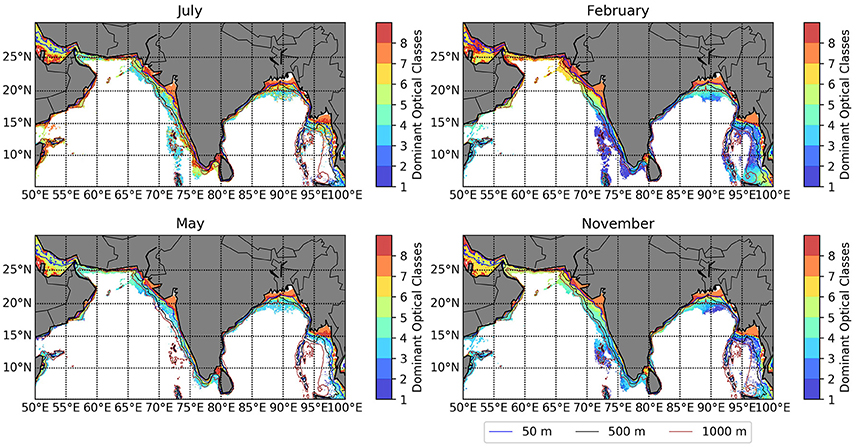
Figure 3. Monthly climatologies of dominant classes (classes of maximum memberships) in the coastal waters of the Northern Indian Ocean. (Top left) July, representative of southwest monsoon season. (Top right) January, representative of northeast monsoon season. (Bottom left) May, representative of Spring intermonsoon season. (Bottom right) November, representative of Fall intermonsoon season. All monthly climatalogies are calculated for the years 1998–2013.

3.3. Spatio-Temporal Variations of Optical Classes in the Northern Indian Ocean

3.3.1. Classes 1 and 2

Optical classes 1 and 2 vary strongly with season. They occur along with class 3 over deeper waters (>200 m). During the southwest monsoon season (June–September), these classes represent very few pixels in deeper waters near the Andaman Sea. In the intermonsoon period (October–November) and northeast monsoon (December–March), classes 1 and 2 are present in the deeper waters along the Southwest coast, West Bengal, and Andaman Sea. The Eastern India coastal current carries the low salinity waters (Optical classes 1 and 2) of the Bay of Bengal to the southwest coast of India during the months of February and March in the winter monsoon season. In the months of March and April, the nearshore waters of the Somalia coast and Gulf of Aden are represented by optical classes 1 and 2, extending to the Gulf of Yemen and Oman. The region 17–20° N, 69–72° E (deeper waters) was also characterized by classes 1, 2, and 3 during the transition period (April–May). The Chlorophyll concentration corresponding to these classes ranged from 0 to 0.2 mg m⁻³ and the optical diversity index fell in the range from 1 to 1.3.

3.3.2. Classes 3 and 4

Optical classes 3 and 4 occurs in the isobaths of 100–2,000 m (shallow to deeper depths). These classes show irregular boundaries in the offshore waters during southwest monsoon season along west and east coasts of India, extending to the deeper waters of Andaman Sea. The classes are found near Gulf of Aden and Oman waters only in June, i.e., during the onset of southwest monsoon. In the autumn intermonsoon (October–November), the classes were distributed over the shallow depths (0–500 m) along the near-shore waters of Gulf of Yemen, Oman, Arabian Sea, and Bay of Bengal. In the northeast monsoon, these classes occurred around the islands off Somalia coast, Gulf of Yemen, west coast, and east coast of India. The Gulf of Oman waters flowing toward the Arabian Sea represents class 4 in May (spring intermonsoon). Chlorophyll concentration corresponding to these classes fell in the range of 0.5–0.75 mg m⁻³ and the diversity index ranged from 0.3 to 0.9.

3.3.3. Class 5

This optical class dominates in regions with isobaths of <1,000 m but >200 m. During the onset of southwest monsoon, class 5 is prominent in the inner Persian Gulf, Strait of Hormuz, Gulf of Oman, Somalia, west and east coasts of India. At the end of southwest monsoon season and onset of the fall intermonsoon period, this class is distributed throughout the coastline in the depth range 0–500 m. This trend persists until the month of January (northeast monsoon) along the entire coastline. In the spring intermonsoon this class is present toward the Persian Gulf, Gulf of Oman flowing into the Northwest coast and further extending toward the east coast of India including the Andaman Sea. This class has chlorophyll levels ranging from 0.75 to 1 mg m⁻³ and the diversity index falls between 0.2 and 0.8.

3.3.4. Classes 6–8

Classes 6–8 dominate in the regions with depths <200 m. Class 6 is dominant in the Persian Gulf characterized by high dense saline waters in all the seasons. Chlorophyll concentration of regions with class 6 varied from 1 to 1.5 mg m⁻³. Classes 7 and 8 are present in the inner shelf regions with shallower depths influenced by boundary currents and river influx. These classes appear in the near-shore waters off the Somalia coast, Gulf of Oman, Inner Gulf of Kutch and Khambhat, Inner Ganges shelf, and Irrawady river basin near Andaman Sea. Local wind-driven circulation brings in the waters of optical classes 7 and 8 from the major river deltas and minor rivers. The influxes from rivers are seasonally variable and rain-fed according to changing precipitation. In the northeast monsoon, waters belonging to classes 7 and 8 flow toward the Strait of Hormuz and into the Arabian Sea in the months of December to April under the influence of strong northwest wind during winter monsoon (Hunter, 1983), turning the Gulf of Oman waters into classes 7 and 8 in February. These classes do not show major variations in the transition periods. The chlorophyll concentration in the regions with classes 7 and 8 was high, ranging from 2 to 2.5 mg m⁻³. The diversity index of the classes 6–8 were low, around 0.3.

3.4. Optical Diversity Index

The previous section describes the distribution of the dominant classes, but contains no information on contributions to the optical signal from non-dominant classes. The optical diversity index, which depends on membership of all classes represented in a pixel provides complementary information on the extent to which non-dominant classes are contributing to the signal. If a single class contributed to the optical signal of a pixel, then the optical diversity would be a minimum of 0.26 in our classification with 8 classes represented. On the other hand, if all classes contributed equally, then the optical diversity index would reach a maximum of 2.08.

The optical diversity index H (Equations 4 and 5) was calculated for all months to study the seasonal and regional variations in optical diversity. The optical diversity index H (Figure 4) fell mostly between 0.3 and 1.36. Regardless of season, higher H values (1–1.36) were found in deeper waters off the south west coast of India (6–15° N), around Lakshadweep and Maldive Islands in the Arabian Sea, around Andaman and Nicobar Islands in the Bay of Bengal and off Myanmar. The highest H values are found in these locations during the winter or northeast monsoon season (December–March), when the areas covered by high H values were also more extensive. High diversity indices were also found in the fall intermonsoon and spring intermonsoon periods. During the summer monsoon season (June–September), the diversity index lay mostly in the 0.5–1 range along the entire study region with some pixels having index >1 appearing in the deeper waters. High diversity indices (1–1.36) occur along the productive upwelling areas, the transition zones between coast and open ocean, oligotrophic waters and regions with the influence of boundary currents. Low diversity indices occur in the regions of most turbid waters, regions of high river water influx and inland waters.

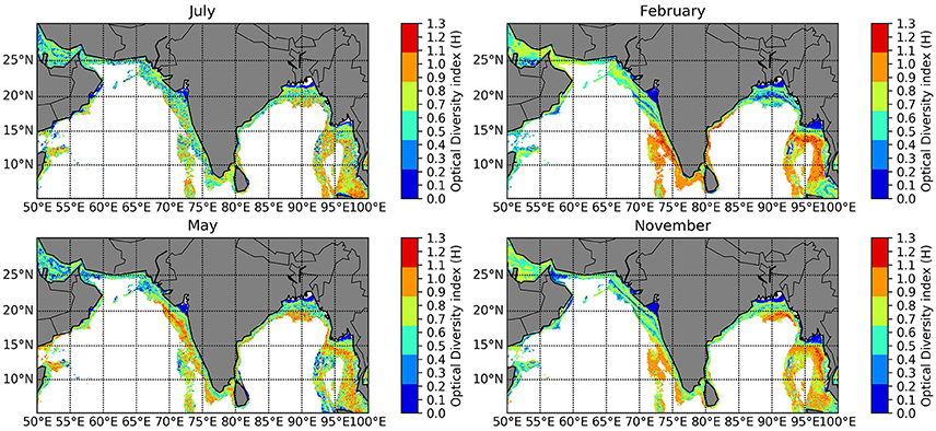
Figure 4. Monthly climatologies of Optical diversity index in the coastal waters of the Northern Indian Ocean. (Top left) July, representative of southwest monsoon season. (Top right) January, representative of northeast monsoon season. (Bottom left) May, representative of Spring intermonsoon season. (Bottom right) November, representative of Fall intermonsoon season. All monthly climatalogies are calculated for the years 1998–2013.

3.5. Optical Classes, Optical Diversity, and Chlorophyll Concentration

In coastal waters, we know that the optical remote-sensing reflectance spectra are affected not only by chlorophyll concentration, but also by suspended sediment load. The seasonal variability of the chlorophyll concentration for the representative months is shown in Figure 5. The remote-sensing reflectance value at 670 nm is often taken to be a measure of suspended sediment load. Therefore, in Figure 6, we have plotted the dominant optical class as a function of chlorophyll-a concentration and R_rs(670), for the monthly climatology of February, as an example. Only well-classified pixels (cumulative class membership >0.5) are plotted. We see a gradual progression in the optical classes 1–8, with increasing chlorophyll concentration and increasing R_rs values, clearly indicating that the optical classification is affected by both chlorophyll concentration and suspended sediment load. Since the chlorophyll concentration in Version 2 of OC-CCI was calculated with a single, global algorithm, we can discount the possibility that the relationship seen in Figure 6 is emerging from the use of different algorithms for different optical classes. On the other hand, it is worth discussing whether a single chlorophyll algorithm would work equally well in all optical classes in the coastal waters of the northern Indian Ocean. Tilstone et al. (2011) reported that there was a good agreement between OC4v6 and another algorithm (OC5) in open-ocean and coastal waters with chlorophyll concentration up to 2 mg m⁻³ for the Arabian Sea and the Bay of Bengal. In the current study, the classes 7 and 8 had chlorophyll concentrations ranging from 1.5 to 2.5 mg m⁻³, quite close to conditions discussed by Tilstone et al. (2011), so that we can assume that OC4 algorithm was suitable for even these high-turbid classes. Nevertheless, it would be interesting, in a future study, to explore the advantages of using algorithms designed for coastal waters (e.g., Le et al., 2013; Loisel et al., 2017; Tilstone et al., 2017).

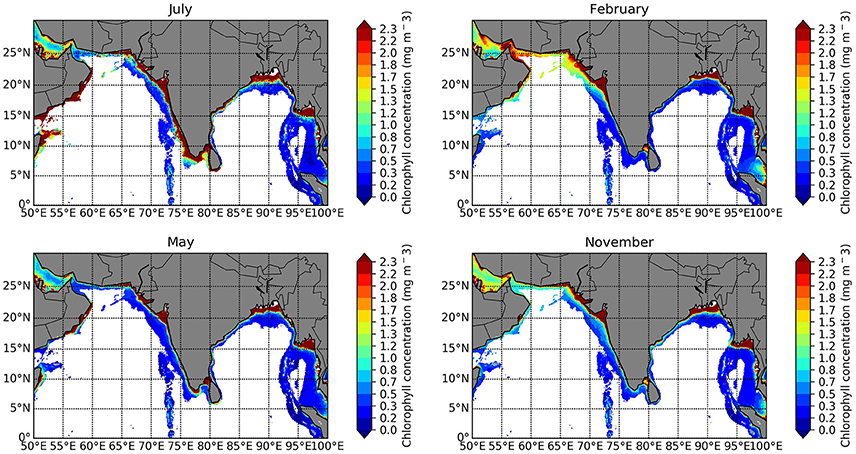
Figure 5. Monthly climatologies of chlorophyll concentrations in the coastal waters of the Northern Indian Ocean. (Top left) July, representative of southwest monsoon season. (Top right) January, representative of northeast monsoon season. (Bottom left) May, representative of Spring intermonsoon season. (Bottom right) November, representative of Fall intermonsoon season. All monthly climatalogies are calculated for the years 1998–2013.

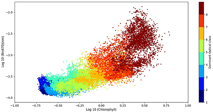
Figure 6. Relationship between chlorophyll concentration and R_rs(670). Climatological data for February are shown as an example. Only well-classified pixels (cumulative membership >0.5) are plotted here. The dominant optical classes are identified using different colors.

A similar plot (Figure 7) for the optical diversity index H reveals a more complex pattern, with very high and very low indices appearing in close juxtaposition to each other in clear waters (where both chlorophyll concentration and R_rs values are low). Strands of high values of the index also appear for higher values of chlorophyll concentration and R_rs. The differences in the distribution of H values, compared with Figure 6 for the optical classification, suggest that optical diversity H perhaps tends to be high during transition between optical classes.

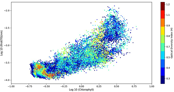
Figure 7. Relationship between chlorophyll concentration and R_rs(670). Climatological data for February are shown as an example. Only well-classified pixels (cumulative membership >0.5) are plotted here. The optical diversity indices are identified using different colors.

3.6. Comparison of Regional Optical Classes With Results of a Global Classification

The question remains whether the regional classification presented here yields results similar to those found in the global classification of Mélin and Vantrepotte (2015). The first difference we note is that the regional classification yielded only eight classes, whereas the global classification produced 16 distinct classes. The log-normalized mean reflectance spectra (Figure 2) of our optical classes 1–4 are similar to those of classes 10–16 of Mélin and Vantrepotte (2015). The spectral characteristics of their classes 8–16 of Mélin and Vantrepotte (2015) are typical of clear waters, and are similar to those of our classes 1 and 2. We also see similarities between the optical signatures of our classes 6, 7, and 8 and the classes 1–7 of Mélin and Vantrepotte (2015), and both these sets are typical of highly turbid waters, with mineral particles and dissolved organic matter (Vantrepotte et al., 2012). For the optical diversity, the values of H from this study lie in the range of 0–1.3 which was lower than the range (0–3) reported by Mélin and Vantrepotte (2015) globally. These differences in values of optical diversity are associated, by definition, with the differences in the number of classes, which has a direct impact on the values of optical diversity (Mélin and Vantrepotte, 2015). It is important to note therefore, that the values of optical diversity reported here are not directly comparable with those of Mélin and Vantrepotte (2015). Similarly, the differences in the class numbers have to be accounted for, when comparing our results with those of Mélin and Vantrepotte (2015).

Concluding Remarks

We have implemented an optical classification using a log-transformed, normalized, remote-sensing reflectance (R_rs) datasets, with spatial resolution of 4 km. In this study, eight optical classes were obtained in the coastal waters of the northern Indian Ocean. Seasonally-reversing monsoons are a defining oceanographic characteristic of the Indian Ocean. Here, we have discussed variations in optical classes with reference to the southwest and northeast monsoon seasons of the study region. The distribution pattern of optical classes in the study region showed major variations between seasons. An example is the presence of optical classes 1, 2, 3, and 4 in the latitudes (0–18° N) during December–March, whereas they were not found in the months of June–September. The influence of class 5 in intermediate coastal waters is consistent in all the regions with fewer variations in each month. Class 6 is also a minimal contributor to the coastal waters of India, restricted the Persian Gulf in northeast monsoon season. These patterns show that in southwest monsoon season, the optical constituents of the coastline are affected mainly by precipitation and river water intrusion; this condition is not prevalent in northeast monsoon season. The regional distribution of dominant optical classes, and how they are related to physical and biological oceanographic features and processes, is presented in the Table S3.

We have also used the memberships of different optical classes in a given pixel, to study optical diversity within a pixel. Both the dominant optical class and the optical diversity index appear to be related to the chlorophyll concentration and the remote-sensing reflectance at 670 nm (used here as an index of suspended sediment load), but in quite different ways. Whereas, the dominant optical classes transition in a systematic matter from classes 1 to 8 with increasing concentration of chlorophyll and increasing R_rs 670, the diversity index appears to be high in areas of transition between optical classes. We also see that the diversity index was high in clear waters around coral islands and in deeper waters away from the shore. Since it is well-known that biological diversity tends to be high when chlorophyll concentration is high, these results suggest that optical diversity indices might run counter to biological diversity. This suggestion can only be verified when data on phytoplankton diversity in the study area become available on a systematic, and extensive basis. But once such relationships are established, optical diversity and optical classification would pave the way for mapping biological diversity at large scales, using remote sensing.

We opted for the Ocean Color Climate Change Initiative products for the study, because of the long time series of data available, which would facilitate extension of our work to study trends and inter-annual variability, and also because of the better spatial coverage, especially during the monsoon season. However, the dataset is limited to six SeaWiFS wavebands in the visible, which was dictated by the historical sensor capabilities. The number of wavebands available also determined the extent to which optical diversity could be explored. No doubt as better-resolution data become available over long time scales from missions such as Sentinel 3, which carries the Ocean and Land Color Instrument (OLCI) sensor with 10 wavebands in the visible domain, it would become possible to investigate optical classes and optical diversity with higher spectral resolution, which may reveal additional optical classes which were not captured in the present analysis.

The optical classification presented in this work enables us to study the seasonal dynamics in the bio-optical characteristics of the coastal waters of the Northern Indian Ocean, and how they are related to the physical and biological processes. Spatio-temporal variations of the eight optical classes under the influence of seasonally reversing monsoons were profound. This study will aid as a first step for investigations of the inter-annual variations in distribution of optical classes and their shifts in response to changing climatic conditions such as El Niño and La Niña events.

Author Contributions

SM: analyzed the datasets, ran the algorithms, and worked on interpretation of the results; TP and SS: implemented and led the study; JJ: assisted with statistical measures used in the study; GG: contributed to the ideas of physical and biological oceanography of the study region; TJ: provided the computational codes for the work. All the authors contributed to the text.

Conflict of Interest Statement

The authors declare that the research was conducted in the absence of any commercial or financial relationships that could be construed as a potential conflict of interest.

Acknowledgments

The authors thank the Department of Science and Technology, Science and Engineering Research Board, India for the Jawaharlal Nehru Science Fellowship to TP. The Director, Central Marine Fisheries Research Institute, India is acknowledged for the support and facilities to pursue this work. The study also contributes to the Ocean Color Climate change Initiative (OC-CCI) of the European Space Agency. This is also a contribution to the activities of the National Centre for Earth Observations of the Natural Environment Research Council of the United Kingdom. We thank Dr. Tim Moore, Research Assistant Professor, University of New Hampshire, for providing the classification algorithm. We also thank Dr. Mike Grant, Plymouth Marine Laboratory, United Kingdom, Mr. Devi Varaprasad and Mr. Abhinav, National Remote Sensing Center, India, Mr. Tarun Joseph, Cochin University of Science and Technology, India and Mr. Muhammad Shafeeque, Central Marine Fisheries Research Institute, India for their extended support in programming and computation.

Supplementary Material

The Supplementary Material for this article can be found online at: https://www.frontiersin.org/articles/10.3389/fmars.2018.00087/full#supplementary-material

References

Antony, M. K., Swamy, G. N., and Somayajulu, Y. K. (2002). Offshore limit of coastal ocean variability identified from hydrography and altimeter data in the eastern Arabian Sea. Cont. Shelf Res. 22, 2525–2536. doi: 10.1016/S0278-4343(02)00100-0
Babin, M., Stramski, D., Ferrari, M. G., Claustre, H., Bricaud, A., Obolensky, G., et al. (2003). Variations in the light absorption coefficients of phytoplankton, nonalgal particles, and dissolved organic matter in coastal waters around Europe. J. Geophys. Res. 108:C7. doi: 10.1029/2001JC000882
Bezdek, J. C., Ehrlich, R., and Full, W. (1984). FCM: the fuzzy c-means clustering algorithm. Comput. Geosci. 10, 191–203.
Brewin, R. J. W., Sathyendranath, S., Müller, D., Brockmann, C., Deschamps, P.-Y., Devred, E., et al. (2015). The ocean colour climate change initiative: III. A round-robin comparison on in-water bio-optical algorithms. Remote Sens. Environ. 162, 271–294. doi: 10.1016/j.rse.2013.09.016
Deborah, J. L., Baskaran, R., and Kannan, A. (2010). A survey on internal validity measure for cluster validation. Int. J. Comput. Sci. Eng. Surv. 1, 85–102. doi: 10.5121/ijcses.2010.1207
Dowell, M., and Platt, T. (2009). Partition of the Ocean into Ecological Provinces: Role of Ocean-Colour Radiometry. International Ocean-Colour Coordinating Group.
Garaba, P. S., and Zielinski, O. (2013). Comparison of remote sensing reflectance from above-water and in-water measurements west of Greenland, Labrador Sea, Denmark Strait, and west of Iceland. Opt. Express 21, 15938–15950. doi: 10.1364/OE.21.015938
Guzman, J. B., Claustre, H., and Marty, J. C. (1995). Specific phytoplankton signatures and their relationship to hydrographic conditions in the coastal northwestern Mediterranean Sea. Mar. Ecol. Prog. Ser. 124, 247–258.
Halkidi, M., Batistakis, Y., and Vazirgiannis, M. (2001). On cluster validation techniques. J. Intell. Inform. Syst. 17, 107–145.
Hunter, J. R. (1983). Aspects of the Dynamics of the Residual Circulation of the Arabian Gulf. Anglesey: Plenum Press.
Jeffries, C. T., Ostrowski, M., Williams, B. R., Xie, C., Jensen, R. M., Grzymski, J. J., et al. (2015). Spatially extensive microbial biogeography of the Indian Ocean provides insights into the unique community structure of a pristine coral atoll. Sci. Rep. 5:15383. doi: 10.1038/srep15383
Karl, D. M., Leteller, R., Hebel, D., Tupas, L., Dore, J., Christian, J., and Winn, C. (1995). Ecosystem changes in the Pacific subtropical gyre attributed to the 1991-1992 El Niño. Nature 373, 230–234.
Krishnamurthy, K., Naidu, W. D., and Santhanam, R. (1978). Plankton biogeography of the Indian Ocean. Int. Rev. Gesamten Hydrobiol. 63, 721–726.
Le, C., Hu, C., Cannizzaro, J., English, D., Muller-Karger, F., and Lee, Z. (2013). Evaluation of chlorophyll-a remote sensing algorithms for an optically complex estuary. Remote Sens. Environ. 129, 75–89. doi: 10.1016/j.rse.2012.11.001
Loisel, H., Vantrepotte, V., Ouillon, S., Ngoc, D. D., Herrmann, M., Tran, V., et al. (2017). Assessment and analysis of the chlorophyll-a concentration variability over the Vietnamese coastal waters from the MERIS ocean color sensor (2002–2012). Remote Sens. Environ. 190, 217–232. doi: 10.1016/j.rse.2016.12.016
Mélin, F., and Vantrepotte, V. (2015). How optically diverse is the coastal ocean?. Remote Sens. Environ. 160, 235–251. doi: 10.1016/j.rse.2015.01.023
Moore, T. S., Campbell, J. W., and Dowell, M. D. (2009). A class-based approach to characterizing and mapping the uncertainty of the MODIS ocean chlorophyll product. Remote Sens. Environ. 113, 2424–2430. doi: 10.1016/j.rse.2009.07.016
Moore, T. S., Campbell, J. W., and Feng, H. (2001). A fuzzy logic classification scheme for selecting and blending satellite ocean color algorithms. Remote Sens. Environ. 39, 1764–1776. doi: 10.1109/36.942555
Morel, A., and Prieur, L. (1977). Analysis of variations in ocean color. Limnol. Oceanogr. 22, 709–722.
Obura, O. D. (2012). The diversity and biogeography of Western Indian Ocean Reef-Building Corals. PLoS ONE 9:e45013. doi: 10.1371/journal.pone.0045013
Obura, O. D. (2016). An Indian Ocean centre of origin revisited: Palaeogene and Neogene influences defining a biogeographic realm. J. Biogeogr. 43, 229–242. doi: 10.1111/jbi.12656
O'Reilly, E. J., Maritorena, S., Mitchell, G. B., Siegel, A. D., Carder, K. L., Garver, S. A., et al. (1998). Ocean color chlorophyll algorithms for SeaWiFS. J. Geophys. Res. 103, 937–953.
Platt, T., and Sathyendranath, S. (1999). Spatial structure of pelagic ecosystem processes in the global ocean. Ecoystems 2, 384–394.
Platt, T., and Sathyendranath, S. (2008). Ecological indicators for the pelagic zone of the ocean from remote sensing. Remote Sens. Environ. 112, 3426–3436. doi: 10.1016/j.rse.2007.10.016
Prieur, L., and Sathyendranath, S. (1981). An optical classification of coastal and oceanic waters based on the specific spectral absorption curves of phytoplankton pigments, dissolved organic matter, and other particulate materials. Limnol. Oceanogr. 26, 671–689.
Qasim, S. Z. (1999). Some unique characteristics of the Indian Ocean. Qatar Univ. Sci. J. 6, 111–116.
Reygondeau, G., Longhurst, A., Martinez, E., Beaugrand, G., Antoine, D., and Maury, O. (2013). Dynamic biogeochemical provinces in the global ocean. Global Biogeochem. Cycles 27, 1–13. doi: 10.1002/gbc.20089
Roxy, M. K., Modi, A., Murtugudde, R., Valsala, V., Panickas, S. S., Kumar, P., et al. (2016). A reduction in marine primary productivity driven by rapid warming over the tropical Indian Ocean. Geophs. Res. Lett. 43, 826–833. doi: 10.1002/2015GL066979
Sathyendranath, S., Brewin, R. J. W., Jackson, T., Melin, F., and Platt, T. (2017). Ocean-colour products for climate-change studies: what are their ideal characteristics. Remote Sens Environ. 203, 125–138. doi: 10.1016/j.rse.2017.04.017
Sathyendranath, S., Groom, S., Grant, M., Brewin, R. J. W., Thompson, A., et al. (2016). ESA Ocean Colour Climate Change Initiative (Ocean-Colour-CCI): Version 2.0 Data. Centre for Environmental Data Analysis.
Schills, T., and Wilson, S. (2006). Temperature threshold as a biogeographic barrier in northern Indian Ocean macroalgae. J. Phycol. 42, 749–756. doi: 10.1111/j.1529-8817.2006.00242.x
Schott, F. A., and McCreary, J. P. (2001). The monsoon circulation of the Indian Ocean. Progr. Oceanogr. 51, 1–123. doi: 10.1016/S0079-6611(01)00083-0
Schott, F. A., Xie, S. P., and McCreary, J. P. Jr. (2009). Indian Ocean circulation and climate variability. Rev. Geophys. 47, 1–46. doi: 10.1029/2007RG000245
Shannon, C. E. (2001). A Mathematical Theory of Communication. New York, NY: ACM SIGMOBILE Mobile Computing and Communications.
Shetye, S., and Shenoi, S. S. C. (1988). Seasonal cycle of surface circulation in the coastal north indian ocean. Proc. Indian Acad. Sci. 97, 53–62.
Shetye, S. R. (1998). West India coastal current and Lakshadweep high/low. Indian Acad. Sci. Limnol. Oceanogr. 23, 637–651.
Tilstone, G., Angel-Benavides, I. M., Pradhan, Y., Shutler, J. D., Groom, S., and Sathyendranath, S. (2011). An assessment of chlorophyll-a algorithms available for SeaWiFS in coastal and open areas of the Bay of Bengal and Arabian Sea. Remote Sens. Environ. 115, 2277–2291. doi: 10.1016/j.rse.2011.04.028
Tilstone, G., Mallor-Hoya, S., Gohin, F., Couto, A. B., Sá, C., Goela, P., et al. (2017). Which ocean colour algorithm for MERIS in NorthWest European waters? Remote Sens. Environ. 189, 132–151. doi: 10.1016/j.rse.2016.11.012
Tomczak, M., and Godfrey, J. S. (2001). Regional Oceanography: An Introduction. Oxford, UK: Elsevier Science Ltd.
Vantrepotte, V., Loisel, H., Dessailly, D., and Meriaux, X. (2012). Optical classification of contrasted coastal waters. Remote Sens. Environ. 123, 306–323. doi: 10.1016/j.rse.2012.03.004
Vinayachandran, P. N., and Shetye, S. R. (1991). The warm pool in the Indian Ocean. Proc. Indian Acad. Sci. 100, 165–175.
Xie, X. L., and Beni, G. (1991). A validity measure for fuzzy clustering. Pattern Anal. Mach. Intell. 13, 841–847.
Keywords: coastal ecosystems, satellite ocean color, classification, remote sensing reflectance, ecosystem management
Citation: Monolisha S, Platt T, Sathyendranath S, Jayasankar J, George G and Jackson T (2018) Optical Classification of the Coastal Waters of the Northern Indian Ocean. Front. Mar. Sci. 5:87. doi: 10.3389/fmars.2018.00087
Received: 30 March 2017; Accepted: 02 March 2018;
Published: 20 March 2018.
Edited by:
Hervé Claustre, Centre National de la Recherche Scientifique (CNRS), FranceReviewed by:
Pierre Gernez, University of Nantes, FranceAneesh Lotliker, Indian National Centre for Ocean Information Services, India
Copyright © 2018 Monolisha, Platt, Sathyendranath, Jayasankar, George and Jackson. This is an open-access article distributed under the terms of the Creative Commons Attribution License (CC BY). The use, distribution or reproduction in other forums is permitted, provided the original author(s) and the copyright owner are credited and that the original publication in this journal is cited, in accordance with accepted academic practice. No use, distribution or reproduction is permitted which does not comply with these terms.
*Correspondence: Grinson George, grinsongeorge@gmail.com