LSTM Neural Network Based Forecasting Model for Wheat Production in Pakistan

Abstract

Pakistan’s economy is largely driven by agriculture, and wheat, mostly, stands out as its second most produced crop every year. On the other hand, the average consumption of wheat is steadily increasing as well, due to which its exports are not proportionally growing, thereby, threatening the country’s economy in the years to come. This work focuses on developing an accurate wheat production forecasting model using the Long Short Term Memory (LSTM) neural networks, which are considered to be highly accurate for time series prediction. A data pre-processing smoothing mechanism, in conjunction with the LSTM based model, is used to further improve the prediction accuracy. A comparison of the proposed mechanism with a few existing models in literature is also given. The results verify that the proposed model achieves better performance in terms of forecasting, and reveal that while the wheat production will gradually increase in the next ten years, the production to consumption ratio will continue to fall and pose threats to the overall economy. Our proposed framework, therefore, may be used as guidelines for wheat production in particular, and is amenable to other crops as well, leading to sustainable agriculture development in general.

1. Introduction

Agriculture sector, being the backbone of Pakistan’s economy, accounted for 19.5 percent of GDP and 42.5 percent of employment in the financial year 2016–2017 [1]. Wheat stood out as the second largest crop; alone responsible for 1.9 percent in the GDP, and 3.4 percent in the employment during the said year. Considering the fact that domestic consumption of wheat continues to increase steadily, its exports are expected to be affected significantly in the coming years, which will be a major setback for the country’s economy. Wheat production forecasting for many years to come is one way of alleviating this predicament; an analysis of its production to consumption ratio will not just be means of estimating the expected amount of export, but will motivate certain measures to be taken at state level to ensure its escalated cultivation, and to minimize losses due to diseases by modern technological methods [2].

The primary objective of a forecasting method is to use several parameters to formulate a mathematical model that predicts the production in future. One such method was presented [3], in which the used parameters included rainfall, temperature, fertilizer, area, and most importantly history of the production. However, the data used in that work was for years 1979–2006, due to unavailability of several parameters until 1979, and the results were verified for only two years. Therefore, the limited dataset comprised wheat production for only 39 years. Moreover, some parameters had to be interpolated to overcome the deficiency in their dataset, which must have contributed to the constrained accuracy they had achieved. We believed that the amount of data available to the authors of [3] was not sufficient for an effective training of any regression model available, therefore, elevating the accuracy to an acceptable level, required a different technique altogether.

It is very difficult to know complete details of these parameters, however, a realistic design approach in this regard is to developing a time series based prediction model, such as auto regressive integrated moving average (ARIMA) model, which is very popular and has shown good results. Several studies have been conducted in the past for wheat forecasting, keeping in view the fluctuations in its production that Pakistan has seen over the years. The most notable studies amongst those were carried out by Amin et al. [4] and Iqbal et al. [5]. In the former, the authors made use of two commercially available software; namely JMP and Statgraphics, and they used time series ARIMA model. They established that the ARIMA (1,2,2) was the best model according to two important model selection criteria, i.e., Akaike’s information criteria (AIC) and Schwarz Bayesian Information criteria (SBIC). The forecasting results showed a root mean squared error (RMSE) of 1145 thousand tons, which reflects a very high prediction error. Due to their linear behavior, ARIMA models prove unsuitable for many real-world nonlinear problems.

The emergence of artificial neural networks (ANN), however, has lightened up the prediction and forecasting fields. ANN have been widely used for prediction of various complex systems [6,7,8,9]. They have capabilities of identifying and learning complex nonlinear relationships between different systems’ parameters, and mostly yield more accurate results when compared with linear regression techniques [10,11]. Amongst various known for long, one recently proposed deep learning architecture of ANN, called Long Short Term Memory Neural Networks (LSTM-NN), has caught attention for time series forecasting [12]. The predictions by this class are influenced by the past behavior of the system, and it can be used for both regression and classification purposes. Compared to other deep models, such as deep Boltzman machine, graph structured recurrent neural network, and convolutional neural networks, the LSTM-NN based deep learning models perform significantly better [13] for time-series forecasting due to set of reasons. It has natural tendency to extract robust patterns for an input feature space, and can handle MIMO systems effectively by offering a lot of system’s flexibility. Additionally, LSTM systems are capable of handling nonlinear systems due to their specialized LSTM nodes that perform better after learning.

LSTM-NN have shown improved modeling capabilities in various time series applications, including stock returns in China [14], traffic dynamics [15], and rent payment delays by tenants [16].

Despite having excellent forecasting capabilities, ANN and LSTM-NN have had limited application in the field of agriculture and crop production forecasting. In [17,18], a recurrent neural network (RNN) based forecasting models were presented for crop yield prediction. In our work, we have used MATLAB 2018^® with deep learning toolbox to develop the wheat production forecasting model. We have adopted the historical data of wheat production for years 1902–2018, and compared the results with existing literature. We have also devised a mechanism, using a smoothing function, to pre-process the dataset prior to training the LSTM-NN model. Our results suggest better forecasting with smaller prediction error. The contribution of this work, therefore, is the recommendation of data pre-processing using a suitable smoothing function in conjunction with the LSTM-NN model, with aim of providing better wheat production forecast.

The rest of the paper is organized as follows: A brief introduction of the ANN and LSTM-NN is given in Section 2. The pre-processing methodology, and training of the LSTM-NN are explained in Section 3. Section 4 presents our simulation results and a comparisons. Section 5 concludes the paper.

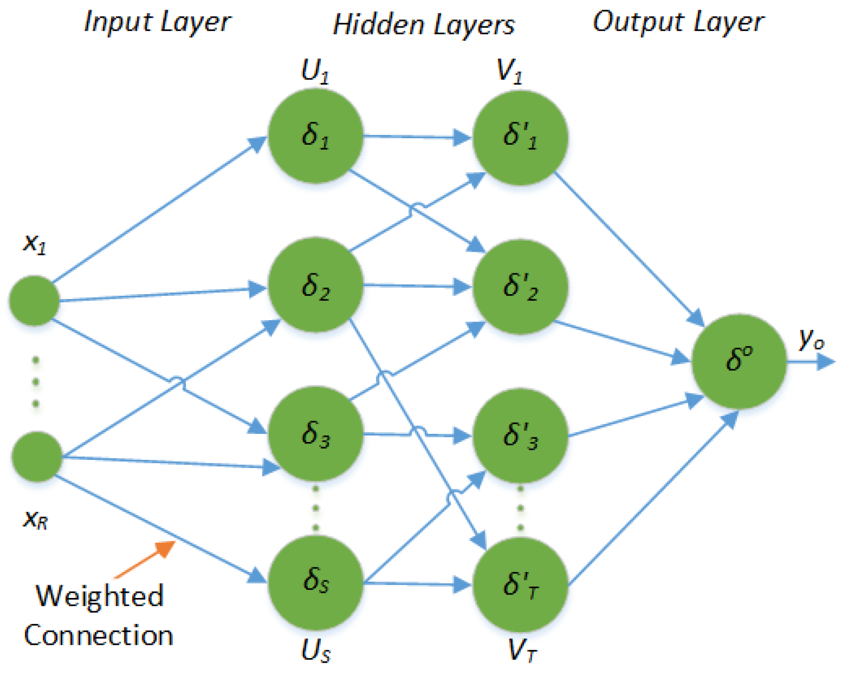
2. Artificial Neural Networks and Long Short Term Memory Neural Networks

The basic concept of ANN is inspired from the neural system of humans [19], where neurons are connected to each other forming a layered structure from inputs to outputs via a few hidden layers. The interconnections between neurons are assigned some weights and biases, together called network’s coefficients. Figure 1 presents an abstract level diagram of ANN, having a set of inputs $(x_1,x_2,...,x_R)$, an output $(y_o)$, and two hidden layers. ${\delta }_i$ and ${\delta }_i^{\prime }$ in the hidden layers are called threshold or quantization functions. Several options are available for thresholding in literature; we have selected log-sigmoid in both hidden layers $(\delta (x)=\frac{1}{1+e^{-x}})$, and purlin in the output layer $(\delta (x)=x)$. ANN have been widely adopted for system modeling, where they are first trained by means of a learning algorithm, in which the network’s coefficients are updated iteratively. The trained model is then used for achieving the desired behavior. One of the most common learning algorithm is back propagation, in which the error is propagated backward.

There are various kinds of ANN architectures; the most common of them are feed-forward, cascaded and recurrent. RNN are widely used for time series forecasting, in which each layer poses some recurrent connections having some unit delays. This results in influence of the current output by previous states. The basic architecture of RNN is shown in Figure 2, where a feedback path exists between second and first hidden layer, $(R_s^{VU})$. One special type of RNN is the LSTM-NN. LSTM-NN are capable of learning long term dependencies in data. The basic concept of LSTM-NN was proposed in [12], and they are now widely applied in various applications. Although RNN are also capable of learning long term dependencies in data, but they suffer from the vanishing gradient issue. LSTM-NN architecture is based on gates, whose function is to choose the data to keep and to discard. Due to gradient control, it can remember more data than RNN. An LSTM-NN cell consists of three gates: input gate, output gate and forget gate. The input gate gives new inputs to the cell. The output gate specifies the output of the cell, and forget gate is responsible for specifying the prior values that need to be retained for future reference. A typical LSTM-NN cell structure is shown in Figure 3.

The gates in the LSTM-NN cell structure are represented by circles in Figure 3. Here g, i, o and f represent modulation gate, input gate, output gate and forget gate respectively. In the modulation gate, the input is updated at the present time instant. All gates work on current input (x(t)) and previous values of states ($h(t-1)$). The outputs of gates are calculated as follows:

$$i(t)=f(W_i{x}_c(t)+U_i{h}_c(t-1)+b_i)$$

(1)

$$g(t)=tanh(W_c{x}_c(t)+U_c{h}_c(t-1)+b_c)$$

(2)

$$g(t)=f(W_f{x}_c(t)+U_f{h}_c(t-1)+b_f)$$

(3)

where, W and U are the weights for input and previous state respectively. The biases are represented with b, subscript is used to represent the specific gate. The updated cell value is calculated as:

$$c(t)=f(W_o+x_c(t)+U_o{h}_c(t-1)+V_{o}c(t)+b_o)$$

(4)

The current cell state, current input and previous state of the cell are used to control the output gate. The updated cell state is given as follows:

$$O(t)=f(W_o{x}_c(t)+U_o{h}_c(t-1)+V_{o}c(t)+b_o)$$

(5)

$$h(t)=O(t)tanh(c(t))$$

(6)

Generally, if hidden layers are more than one the network architecture could be categorized as deep network. In the proposed work, we have evaluated various hidden layers structures in the LSTM-NN to get the best results.

3. Materials and Methods

The proposed research methodology is depicted in Figure 4. Pakistan’s wheat production history for the years 1902–2018, constituting our dataset, was obtained from the Federal Bureau of Statistics, Pakistan, and the Economic Survey of Pakistan, 2017 [1]. The dataset is divided into two subsets: The first subset, comprising data from 1902–2008, is used for training the three forecasting models, namely, ARIMA, RNN and LSTM-NN. The second subset consists of data from 2009–2018, and is used for the validation purpose.

Since, the raw data included fluctuations that might affect the forecasting results, a smoothing function is used to smooth out the curve values prior to training the models. One of the most widely used smoothing functions is Robust-LOWESS [23]. It uses local regression using linear recursive least squares (RLS). The presence of outliers in the data degrades its modeling accuracy. Using the local regression, it decreases the effects of outliers and results in improved modeling. This algorithm assigns very low weights to the outliers. The smoothing function with a polynomial of degree two, and a window size of four years, is used for data pre-processing. Algorithm 1 presents our proposed methodology.

Algorithm 1: Proposed Methodology

All the three models, ARIMA, RNN and LSTM-NN, are then developed using both the raw and the pre-processed data, resulting in a total of six models. The latter are then compared with the actual values in the validation step. We use mean absolute error (MAE), root mean squared error (RMSE) and correlation coefficient value (R-value) as the three performance metrics for comparison. The R-value determines correlation between actual and predicted values. Its value is between 0 and 1, where 0 means no correlation while 1 means a perfect match. Considering x to be the actual values, y representing the predicted values, $\overline{x}$ representing mean of x, $\overline{y}$ representing mean of y and n is number of samples, these metrics are calculated by their standard formulas as given in Equations (7)–(9).

$$MAE={\displaystyle \frac{{\sum }_{i=1}^n|x_i-y_i|}{n}}$$

(7)

$$RMSE=\sqrt{{\displaystyle \frac{{\sum }_{i=1}^n{(x_i-y_i)}^2}{n}}}$$

(8)

$$R={\displaystyle \frac{{\sum }_{i=1}^n(x_i-\overline{x})(y_i-\overline{y})}{\sqrt{{\sum }_{i=1}^n{(x_i-\overline{x})}^2}\sqrt{{\sum }_{i=1}^n{(y_i-\overline{y})}^2}}}$$

(9)

The benchmark model for wheat production forecasting is the ARIMA model [4], denoted as ARIMA (p,d,q) model, where p,d,q are orders of auto regressive, differencing, and moving average models respectively. [4] used the ARIMA models with parameters (1,2,2). There are various variants of RNN in literature [19]; we have selected a nonlinear auto-regressive model (NAR). In ANN there are no specific steps to achieve the best models; instead there are some guidelines that may be followed, such as, increasing the number of hidden layers, and using different training functions to tune our model accuracy [19]. In the development of RNN model having NAR architecture, various tuning parameters were tested. These parameters are given in

Table 1. Parameters used for developing RNN forecasting model.

Parameter	Range	Parameter	Range
Feedback delays	1 to 5	No. of neurons in each hidden layer	1 to 40
No. of Hidden layers	1 to 3	Training functions	Bayesian regularization [19], Levenberg–Marquardt [19]

. The results of each configuration were compared with the actual values and were evaluated on same metrics defined in Equations (7)–(9). MATLAB software’s ANN toolbox is used for all the simulations.

Similarly, a set of tuning parameters was used to build the forecasting model for LSTM-NN; given in

Table 2. Parameters used for developing LSTM-NN forecasting model.

Parameter	Range	Parameter	Range
Hidden Units	1 to 2000	Learn drop rate period	1 to 100
Initial learning rate	0.001 to 0.009	Solver	Adam optimizer [24], stochastic gradient descent with momentum (SGDM) [25]

. As far as selection of the solver is concerned, Adam Optimizer [24] and SGDM [25] have shown excellent suitability for LSTM-NN, which have a gradient control property. However, the better among the two can only be determined for a given dataset, since each of them largely depends upon size of the dataset, and whether the problem has non-stationary objectives and sparse gradients [26]. The accuracy of each solver may differ depending upon the application.

The results of each configuration were compared with the actual values and were evaluated on same metrics defined in Equations (7)–(9). MATLAB software’s Deep learning toolbox is used for all the simulations of LSTM-NN.

4. Results and Discussion

The original time series plot for the wheat production in Pakistan from the year 1902 to 2018 is shown in Figure 5. After applying the smoothing function, a smooth time series curve is achieved as shown in Figure 6. The best values of various tuning parameters of RNN and LSTM-NN are given in

Table 3. Best parameters for RNN and LSTM-NN forecasting models.

RNN				RNN pre-processed
Parameter	Value	Parameter	Value	Parameter	Value	Parameter	Value
Feedback delays	2	No. of neurons in each hidden layer	28,6	Feedback delays	4	No. of neurons in each hidden layer	28,10
No. of Hidden layers	2	Training function	Bayesian regularization	No. of Hidden layers	2	Training function	Bayesian regularization
LSTM-NN				LSTM-NN pre-processed
Parameter	Value	Parameter	Value	Parameter	Value	Parameter	Value
Hidden units	2000	Learn rate drop period	120	Hidden units	200	Learn rate drop period	20
Initial learning rate	0.009	Solver	SGDM	Initial learning rate	0.0032	Solver	SGDM

. These parameters values resulted in achieving minimum MAE, minimum RMSE and highest R-value for each model category. These values were result of rigorous testing of various parameter values for each model.

All the models are trained using the data from year 1902–2008, whereas, the data from 2009–2018 was used for validation. The comparison between step-ahead forecast using the proposed models and that by the existing benchmark model [4], for period 2009–2018, are given in

Table 4. The difference between actual and forecast wheat production (in thousand tons) for years 2009–2018 using various models.

Year	Actual	ARIMA(1,2,2)	ARIMA(1,2,2) Pre-Processed	RNN	RNN Pre-Processed	LSTM-NN	LSTM-NN Pre-Processed
2009	24,033	1688.6	197.7	430.06	2683.32	1382.40	802.89
2010	23,311	434	−1042.1	4213.38	1405.02	304.46	−400.79
2011	25,214	1941.2	349.8	60.18	2620.00	1824.97	1025.45
2012	23,473	−173.7	−1899.5	−761.99	138.64	−284.71	−1180.16
2013	24,211	194	−1668.6	−382.72	176.09	96.99	−893.75
2014	25,979	1592.2	−407.3	1540.87	1337.55	1521.19	436.38
2015	25,086	329.5	−1806.8	581.68	−47.94	296.87	−880.03
2016	25,633	506.8	−1766.2	1156.40	141.09	525.06	−741.32
2017	26,674	1178.1	−1231.6	2185.48	959.31	1259.67	−92.83
2018	26,300	434.4	−2112	1816.46	465.38	591.66	−843.05

. The results shows a significant improvement in terms of wheat production forecasting. The error terms MAE and RMSE, which are widely used to represent the model error, shows that LSTM-NN developed using pre-processed data is the most accurate model. LSTM-NN model developed on pre-processed data has the MAE value of 729 thousand tons, which shows an improvement of about 14% against the existing benchmark model [4]. Similarly, RMSE shows an improvement of 25%. The results of the six models are also compared in term of R-value: the higher the R-Value the higher is the correlation between the actual and the predicted values. The regression plots of all six models along with their R-Values are shown in Figure 7. The dotted line represent the best fit and continuous line is the actual fit between actual and predicted values. ARIMA model based on pre-processed data, LSTM-NN model and LSTM-NN model model developed on pre-processed data have the highest R-value of 0.81. This shows a strong correlation between actual and predicted values. The best results for each model are summarized in

Table 5. Comparison of various forecasting models.

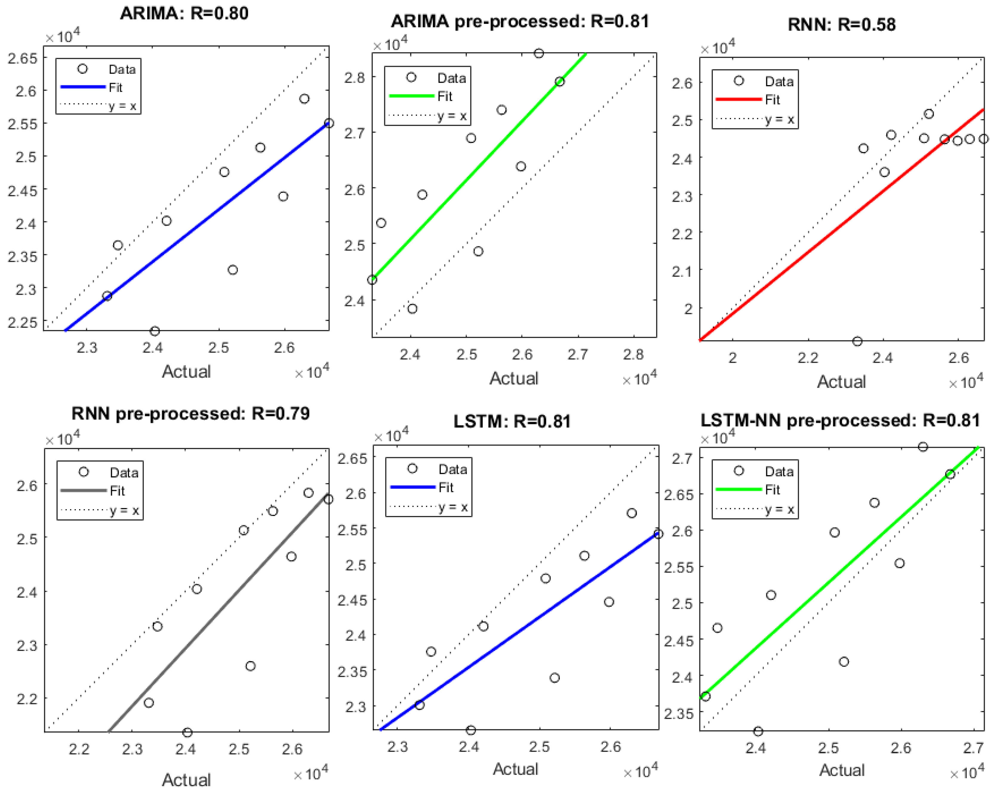
Model	RMSE	MAE	R-Value
ARIMA (1,2,2) [4]	1065	847	0.80
ARIMA (1,2,2) pre-processed	1420	1248	0.81
RNN	1754	1313	0.58
RNN pre-processed	1379	997	0.79
LSTM-NN	1002	808	0.81
LSTM-NN pre-processed	792	729	0.81

. Both LSTM-NN models gave accurate results due to better learning capabilities of LSTM-NN. The results clearly shows that LSTM-NN model developed on pre-processed data gives best results.

The wheat production values using the LSTM-NN model with pre-processed data for future years are given in

Table 6. Ten years ahead wheat production forecasting (in thousand tons) of Pakistan.

Year	Wheat Production Forecast
2019	27,103
2020	27,388
2021	27,657
2022	27,908
2023	28,143
2024	28,362
2025	28,566
2026	28,756
2027	28,933
2028	29,096

. It is forecasted that in 2028, Pakistan annual wheat production will be about 29,096 thousand tons considering consistent social, environmental and economic conditions.

5. Conclusions

In this work we have proposed to use Robust-LOWESS as a smoothing function in conjunction with a LSTM-NN model to predict wheat production in Pakistan for years 2019–2028. We demonstrate that removing the outliers from the original data, prior to performing the actual prediction, helps in improving the accuracy by a significant amount. We have used MATLAB as the simulation tool, and RMSE, MAE and correlation coefficient as the comparison metrics. Our study reveals a significant improvement of in terms of model accuracy in comparison to the existing works. Our study is crucial since Pakistan’s economy immensely depends upon agriculture, and wheat usually stands out as the second most important crop.

References

- Ministry of Food Agriculture. Livestock, Islamabad G.o.P. Economic Survey of Pakistan. 2011. Available online: http://www.finance.gov.pk/survey/chapter_12/02-Agriculture.pdf (accessed on 31 January 2019).
- Akram, T.; Naqvi, S.R.; Haider, S.A.; Kamran, M. Towards real-time crops surveillance for disease classification: exploiting parallelism in computer vision. Comput. Electr. Eng. 2017, 59, 15–26. [Google Scholar] [CrossRef]
- Sher, F.; Ahmad, E. Forecasting Wheat Production in Pakistan. Lahore J. Econ. 2008, 13, 57–85. [Google Scholar]
- Amin, M.; Amanullah, M.; Akbar, A. Time Series Modeling for forecasting wheat production of Pakistan. Plant Sci. 2014, 24, 1444–1451. [Google Scholar]
- Iqbal, N.; Bakhsh, K.; Maqbool, A.; Ahmad, A.S. Use of the ARIMA model for forecasting wheat area and production in Pakistan. J. Agric. Soc. Sci. 2005, 1, 120–122. [Google Scholar]
- Naqvi, S.; Akram, T.; Haider, S.; Kamran, M.; Shahzad, A.; Khan, W.; Iqbal, T.; Umer, H. Precision Modeling: Application of Metaheuristics on Current–Voltage Curves of Superconducting Films. Electronics 2018, 7, 138. [Google Scholar] [CrossRef]
- Haider, S.A.; Naqvi, S.R.; Akram, T.; Kamran, M. Prediction of critical currents for a diluted square lattice using Artificial Neural Networks. Appl. Sci. 2017, 7, 238. [Google Scholar] [CrossRef]
- Naqvi, S.R.; Akram, T.; Haider, S.A.; Kamran, M. Artificial neural networks based dynamic priority arbitration for asynchronous flow control. Neural Comput. Appl. 2018, 29, 627–637. [Google Scholar] [CrossRef]
- Naqvi, S.R.; Akram, T.; Iqbal, S.; Haider, S.A.; Kamran, M.; Muhammad, N. A dynamically reconfigurable logic cell: From artificial neural networks to quantum-dot cellular automata. Appl. Nanosci. 2018, 8, 89–103. [Google Scholar] [CrossRef]
- Rather, A.M.; Agarwal, A.; Sastry, V. Recurrent neural network and a hybrid model for prediction of stock returns. Expert Syst. Appl. 2015, 42, 3234–3241. [Google Scholar] [CrossRef]
- Bengio, S.; Vinyals, O.; Jaitly, N.; Shazeer, N. Scheduled sampling for sequence prediction with recurrent neural networks. In Proceedings of the Advances in Neural Information Processing Systems, Montreal, QC, Canada, 7–12 December 2015; pp. 1171–1179. [Google Scholar]
- Hochreiter, S.; Schmidhuber, J. Long short-term memory. Neural Comput. 1997, 9, 1735–1780. [Google Scholar] [CrossRef] [PubMed]
- Tan, M.; Santos, C.D.; Xiang, B.; Zhou, B. LSTM-based deep learning models for non-factoid answer selection. arXiv, 2015; arXiv:1511.04108. [Google Scholar]
- Chen, K.; Zhou, Y.; Dai, F. A LSTM-based method for stock returns prediction: A case study of China stock market. In Proceedings of the 2015 IEEE International Conference on Big Data (Big Data), Santa Clara, CA, USA, 29 October–1 November 2015; pp. 2823–2824. [Google Scholar]
- Ma, X.; Tao, Z.; Wang, Y.; Yu, H.; Wang, Y. Long short-term memory neural network for traffic speed prediction using remote microwave sensor data. Transp. Res. Part C Emerg. Technol. 2015, 54, 187–197. [Google Scholar] [CrossRef]
- Garn, W.; Hu, Y.; Nicholson, P.; Jones, B.; Tang, H. LSTM network time series predicts high-risk tenants. In Proceedings of the Euro 2018–29th European Conference on Operational Research, EURO 2018, Valencia, Spain, 8–11 July 2018. [Google Scholar]
- Guo, W.W.; Xue, H. Crop yield forecasting using artificial neural networks: A comparison between spatial and temporal models. Math. Probl. Eng. 2014, 2014, 857865. [Google Scholar] [CrossRef]
- Meena, M.; Singh, P.K. Crop Yield Forecasting Using Neural Networks. In International Conference on Swarm, Evolutionary, and Memetic Computing; Springer: Cham, Switzerland, 2013; pp. 319–331. [Google Scholar]
- Schalkoff, R.J. Artificial Neural Networks; McGraw-Hill: New York, NY, USA, 1997; Volume 1. [Google Scholar]
- Hagan, M.T.; Demuth, H.B.; Beale, M.H.; De Jesús, O. Neural Network Design; Pws Pub.: Boston, MA, USA, 1996; Volume 20. [Google Scholar]
- Kamran, M.; Haider, S.; Akram, T.; Naqvi, S.; He, S. Prediction of IV curves for a superconducting thin film using artificial neural networks. Superlattices Microstruct. 2016, 95, 88–94. [Google Scholar] [CrossRef]
- Haider, S.A.; Naqvi, S.R.; Akram, T.; Kamran, M.; Qadri, N.N. Modeling electrical properties for various geometries of antidots on a superconducting film. Appl. Nanosci. 2017, 7, 933–945. [Google Scholar] [CrossRef]
- Cleveland, W.S. LOWESS: A program for smoothing scatterplots by robust locally weighted regression. Am. Stat. 1981, 35, 54. [Google Scholar] [CrossRef]
- Kingma, D.P.; Ba, J. Adam: A method for stochastic optimization. arXiv, 2014; arXiv:1412.6980. [Google Scholar]
- Mandt, S.; Hoffman, M.D.; Blei, D.M. Stochastic gradient descent as approximate Bayesian inference. J. Mach. Learn. Res. 2017, 18, 4873–4907. [Google Scholar]
- Wilson, A.C.; Roelofs, R.; Stern, M.; Srebro, N.; Recht, B. The marginal value of adaptive gradient methods in machine learning. In Proceedings of the Advances in Neural Information Processing Systems, Long Beach, CA, USA, 4–9 December 2017; pp. 4148–4158. [Google Scholar]