
Dual-Branch Deep Convolution Neural Network for Polarimetric SAR Image Classification


1
School of Electronic and Information Engineering, Beihang University, Beijing 100191, China
2
Department of Computer and Electronic Engineering, Wuzhou University, Wuzhou 543000, China
3
Cognitive Signal-Image and Control Processing Research Laboratory, School of Natural Sciences University of Stirling, Stirling FK9 4LA, UK
4
Space Mechatronic System Technology Laboratory, Department of Design, Manufacture and Engineering Management University of Strathclyde, Glasgow G1 1XJ, UK
*
Author to whom correspondence should be addressed.
Appl. Sci. 2017, 7(5), 447; https://0-doi-org.brum.beds.ac.uk/10.3390/app7050447
Submission received: 9 March 2017
/
Revised: 23 April 2017
/
Accepted: 24 April 2017
/
Published: 27 April 2017
(This article belongs to the Special Issue Polarimetric SAR Techniques and Applications)
Abstract
:The deep convolution neural network (CNN), which has prominent advantages in feature learning, can learn and extract features from data automatically. Existing polarimetric synthetic aperture radar (PolSAR) image classification methods based on the CNN only consider the polarization information of the image, instead of incorporating the image’s spatial information. In this paper, a novel method based on a dual-branch deep convolution neural network (Dual-CNN) is proposed to realize the classification of PolSAR images. The proposed method is built on two deep CNNs: one is used to extract the polarization features from the 6-channel real matrix (6Ch) which is derived from the complex coherency matrix. The other is utilized to extract the spatial features of a Pauli RGB (Red Green Blue) image. These extracted features are first combined into a fully connected layer sharing the polarization and spatial property. Then, the Softmax classifier is employed to classify these features. The experiments are conducted on the Airborne Synthetic Aperture Radar (AIRSAR) data of Flevoland and the results show that the classification accuracy on 14 types of land cover is up to 98.56%. Such results are promising in comparison with other state-of-the-art methods.
1. Introduction
Polarimetric synthetic aperture radar (PolSAR) is a kind of high resolution imaging system, which can work under all weather, day-and-night conditions. The PolSAR data can be used to describe the scattering mechanism of the earth surface and provide rich information for terrain surface classification with the complex coherency matrix [1], scattering matrix [2], etc. With the development of the PolSAR system, PolSAR data such as Advanced Synthetic Aperture Radar (ASAR)/Environmental Satellite (ENVI-SAT), Phased Array L-band Synthetic Aperture Radar (PALSAR)/Advanced Land Observing Satellite (ALOS) and Radar Satllite-2 are becoming more and more available, thus PolSAR image classification has become an important research topic [3].
It is a challenge to automatically extract and select features in PolSAR image classification. Traditional methods generally extract features manually per the scattering characteristics of the terrain surface. The features include radiation information [4], polarization information [5], sub-aperture decomposition [6], decomposition information [7], etc. A single feature or combined features are then fed into an appropriate classifier for classification. Using features individually cannot achieve satisfactory performance. Even if these features are combined then, the classification accuracy will not be improved due to subjectiveness. In addition, the features that can be combined are limited, and the computational complexity will grow with the increase of the amount of combined features. Therefore, traditional methods cannot make full use of the rich features of the PolSAR data to improve the classification accuracy.
In recent years, the theory of deep learning has set off a wave in the field of pattern recognition. In 2006, Hinton et al. proposed an unsupervised greedy method based on Deep Belief Network (DBN), which trains layer by layer, solving the vanishing gradient problem caused by deep training [8]. In 2011, Wong et al. proposed the regularized deep Fisher mapping (RDFM) method per Fisher criterion to enhance the feature separability by using the neural network algorithm, which can eliminate the overfitting problem [9]. Then, many scholars put forward a variety of deep learning models based on different application backgrounds, such as Deep Restricted Boltzmann (DRB) [10], Stacked Denoising Autoencoders (SDA) [11], and the Deep Convolutional Neural Network (CNN) [12]. As a pillar of deep learning, the CNN is one of the best models for solving the “perception” issues. For example, the AlexNet model won first prize in the ImageNet ILSVRC image classification contest in 2012, which has caused widespread concern in related fields [13]. To solve the problem of inefficient utilization of features in PolSAR image processing, some scholars introduce the deep learning framework to extract features of PolSAR images. Wang et al. converted the PolSAR image into the scattering matrix, and then established multichannels for the CNN model [14]. Afterwards, the features were extracted automatically and the images were classified by wide training. Experimental results showed that the PolSAR image classification algorithm based on the CNN is higher than that of the traditional algorithms using the same dataset. Zhou et al. converted the complex matrix of the PolSAR image into a real matrix of six channels to suit the input of the neural network, and designed two, cascaded, fully connected networks to map the features to a certain classifier [15]. This algorithm further improves the accuracy of PolSAR image classification.
Although the deep learning framework provides an idea to solve the problem of low utilization of rich features in PolSAR image classification, it still faces the following problems. First, SAR image is a special kind of microwave image and the regions with the same gray level do not necessarily have similar optical properties. Therefore, the existing methods for optical images based on the deep learning framework may not be suitable for PolSAR image processing. Second, the existing PolSAR image classification methods based on deep learning only consider the polarization features of the image, while ignoring the spatial features.
To solve the above problems, this paper proposes a dual-branch deep convolution neural network (Dual-CNN) method for PolSAR image classification. The proposed method is composed of two CNNs: one is used to extract the polarization features of the real matrix of the six channels (6Ch-CNN) and the other is used to extract the spatial features of the Pauli RGB image (PauliRGB-CNN). These two kinds of features are fed into a fully connected layer to achieve mutual harmony, and then the Softmax classifier is followed immediately to complete the classification work.
2. Basics of the CNN
A typical CNN is composed of an input layer, convolution layer, pooling layer and output layer. The input layer receives the pixels from the image. The convolution layer utilizes the convolution kernel to extract image features. The pooling layer is followed by the convolution layer, aiming at reducing the pixels to be processed and formulating the abstract features. The output layer maps the extracted features into classification vectors corresponding to the feature categories. The training of the CNN has two processes: the Forward Propagation and the Backward Propagation.
2.1. The Forward Propagation
The Forward Propagation (FP) is a mapping process where the output of the previous layer is taken as the input of the current layer. To avoid the defects of the linear model, neurons of each layer should be added with a nonlinear activation function in the mapping process. Since the first layer only receives pixel values, there are no activation functions. From the second layer to the last layer, nonlinear activation functions are employed. Thus, the output of each layer can be expressed as:
where l represents the layer, and ∗ means convolution operation. , , and are the weights matrix (for the convolution layer, it is the convolution kernel), the bias matrix and weighted input of the layer respectively. is the nonlinear activation function. If , then is the image matrix whose elements are pixel values. If , then is the feature maps matrix , which is extracted from the layer i.e., . Suppose L is the output layer, represents the final output vector.
2.2. The Backward Propagation
The Backward Propagation (BP) algorithm is a supervised learning method. It first selects a cost function based on the output and the targeted values, then calculates the error vectors, and lastly applies the Gradient Descent (GD) to update and parameters. Specifically:
- Selection of cost function. The quadratic function is the common cost function. However, it would be time-consuming if the neurons make an obvious mistake during the training process. Alternatively, we take Cross-Entropy () as the cost function which is determined by Equation (2):where n is the total number of training sets, and N is the number of neurons in the output Layer corresponding to the N classes. is the targeted value corresponding to the neuron of the output layer, and is the actual output value of the neuron of the output layer.
- Calculation of error vectors. The error vector of the output layer L is defined bywhere the symbolic represents the partial derivative operation. Back-propagate the error vector . For each , can be computed by the Chain Rule as:where the symbolic ∘ is the Hadamard product (or Schur product) which denotes the element-wise product of the two vectors.
- Updates of weights and the bias matrix. The gradients of and are denoted as and respectively. The partial derivative of to and can be calculated with Equations (1) and (3):The change values of and : and , can be calculated respectively bywhere represents the learning rate.
2.3. Feature Extraction
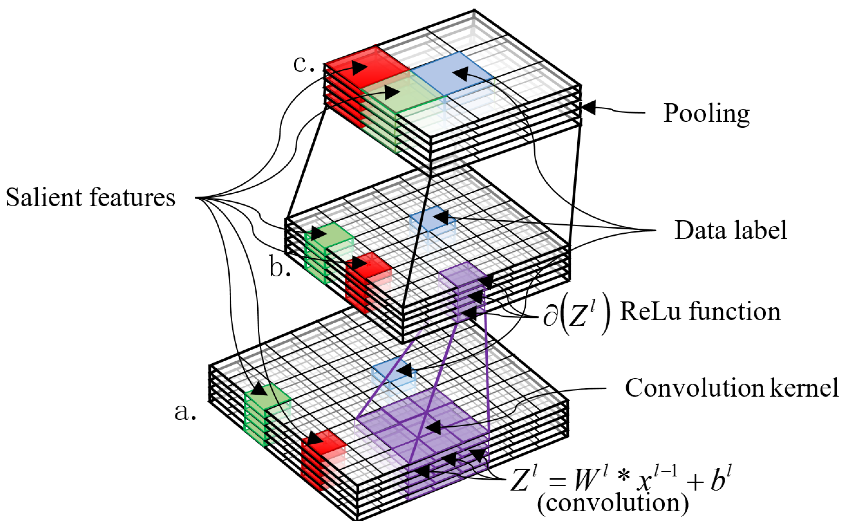
In the training process, the CNN is used to extract the features from the data based on the convolution operation. The convolution operation includes a convolution layer followed immediately by a pooling layer. The feature extraction process is shown in Figure 1. From bottom to top, a represents the input data, b represents the feature data which is obtained by the convolution operation and the ReLu (Rectified Linear Units) activation function, and c represents the feature data which is obtained after the pooling process. Red and green patches represent different salient features, blue patches represent the label of the data(or interesting target), the purple patch in a represents the convolution kernel, and the purple patch in b represents the feature which is obtained from the purple patch in a by the convolution operation and the ReLu activation function. More specifically, the CNN works as follows.
First, the salient features of a are preserved, and then passed to a ReLu function for post processing. Second, the non-salient features of a are filtered out by ReLu via setting the minus in the feature map to 0. The derived features are b. Finally, more abstract features c of the input data will be obtained based on the pooling layer. If features c are not abstract enough, a second convolution operation is needed. The process is repeated until the most representative features are obtained. This results in deepening the layers of the CNN. In the whole process, the data-label of a may be filtered out, but its main neighborhood features can be preserved for judging a-label. In addition, it is worth noting that there is no clear conclusion how many layers of convolution operations are appropriate. Thus, the visual convolution operation is needed.
3. The Proposed Method
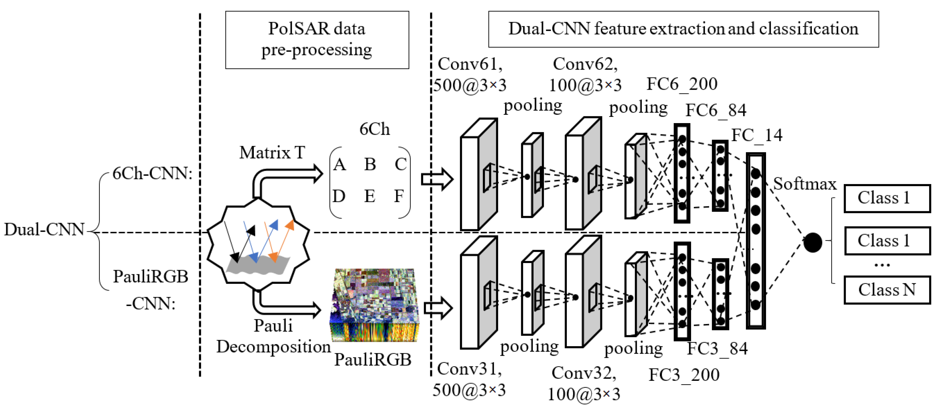
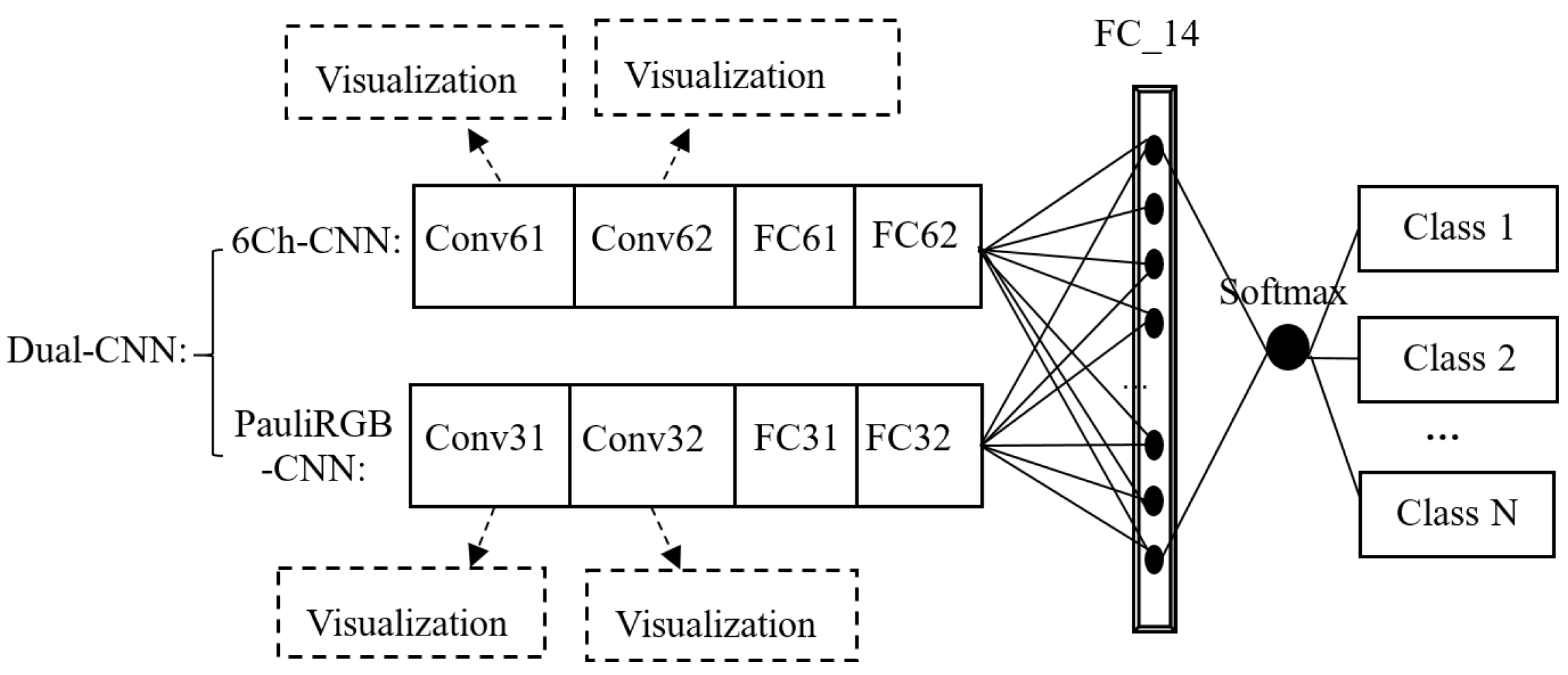
The proposed method consists of two frameworks: PolSAR data pre-processing and Dual-CNN model design. As shown in Figure 2, the Dual-CNN includes the 6Ch-CNN and PauliRGB-CNN. The polarization features and the spatial features are generated from the pre-processed data by the 6Ch-CNN and PauliRGB-CNN; then, these features are combined by a fully connected layer. In this paper, the above combined features are named as P-S features. Finally, the P-S features are classified by the Softmax classifiers.
3.1. PolSAR Data Pre-Processing
Since the obtained PolSAR data contain the complex coherent matrix, they cannot be directly fed into the Dual-CNN model and a pre-processing is required. The pre-processing of the PolSAR data contains three steps: creating a 6Ch to allow the input and representation of polarimetric data; generating a Pauli RGB image to obtain the spatial feature; patching the images with fixed size to adapt to the CNN.
3.1.1. Creating 6Ch to Represent the Polarimetric Data
Under the multi-look and reciprocity assumption, the single station PolSAR can be represented by the 3 × 3 complex coherent matrix T which is symmetrical. To adapt the input format of the convolution neural network, it is necessary to convert the data into a real matrix. We create a 6Ch to represent the polarimetric data, and each channel is obtained by Equation (7):
where , , represent the diagonal elements of the matrix T and they are real numbers while , , represent complex elements. A is the total scattering power in decibels, here ; B and C are normalized power of and ; D, E and F are the relative correlation coefficients. Except A, the remaining five parameters are normalized to [0, 1]. Thus, the PolSAR data are converted into a 6Ch to form a dataset, where 6 represents the total number of the channels, i.e., A, B, C, D, E and F; m and n represent the number of rows and columns in a single channel, respectively.
3.1.2. Generating Pauli RGB Image to Obtain the Spatial Feature
The Pauli decomposition of the scattering matrix S is often employed to represent all the polarimetric information in a single PolSAR image, and its form is:
where , , and constitute a set of orthogonal Pauli bases, and a, b, c and d are coefficients. is the odd scattering mechanism, representing the terrain scattering body; is the dihedral scattering mechanism rotating around the axis, and its echo polarization and incident polarization are on the mirror symmetry; is the dihedral scattering mechanism rotating around the axis, and its echo polarization and incident polarization are orthogonal; is the antisymmetric component. Since the corresponding scattering mechanism does not exist in the nature, the weighted coefficient d is 0 generally. After the Pauli decomposition, the Pauli RGB image is synthetized by a pseudo-color process using the energy corresponding to a, b and c, as is described in Equation (9):
The synthesised Pauli RGB image contains rich contour, texture, and color features, which is in greet agreement with those of real ground scenes. This enables recognition by the naked eye. In addition, the Pauli RGB image can reduce the interference of other data on the feature extraction, improving algorithm robustness. Furthermore, the CNN is good at dealing with color images, so the Pauli RGB image is suitable. For these reasons, many classification algorithms use the Pauli RGB image as their input [16,17], and so does our method.
3.1.3. Patching the Images with Fixed Size
It is required that the CNN processes the data with a fixed size. However, different targets usually have different sizes, so it is difficult to use a generalized size for all target slices. Thus, some researchers propose to process the patches via stretching or filling the bounding of the image with 0 pixels. Although these methods can solve this problem to a certain extent, they will bring some unexpected errors. For example, if the boundary of small objects is filled with 0, the detection accuracy of the targets in complex environments will be limited, which thereby influences its feature learning. The details of our patching method are as follows.
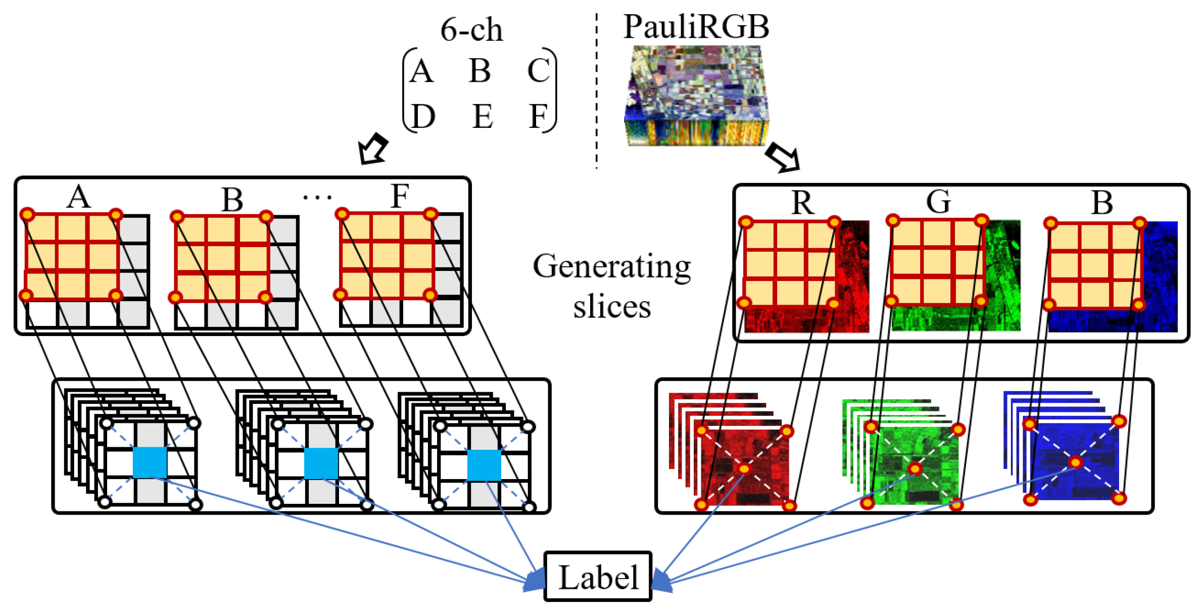
First, based on the sliding window with a fixed size, we traverse the entire dataset to obtain a set of fixed size slices for each channel of the 6Ch and Pauli RGB image, which is shown in Figure 3.
By this way, the maximum number of slices for each channel can be obtained by:
where w and h are the width and height of each channel data respectively, s is the size of the sliding window, and i is the span while sliding. It should be noted that s and i are relevant to the size of the target. If the target is small (e.g., several pixels), then i is minor and s should be carefully selected. The selection of both parameters will be detailed in the experiment section.
Second, we assign a label for each slice. Specifically, each pixel in ground-truth is assigned a label per the category it belongs to, and then we choose the location of the center pixel of the slice as the index to search the category label in the ground-truth. The selected label is finally assigned for the slice.
In this manner, all samples are obtained with labels attached, and we can ensure that the CNN can process the small target in the complex environment.
Using a sliding window can get enough training sets, but the samples will be more or less repeated. Therefore, before feeding the data into the CNN, we need to reduce the data redundancy by principle component analysis (PCA).
3.2. Feature Extraction and Classification Based on the Dual-CNN Model
The Dual-CNN model consists of two CNNs, i.e., the 6Ch-CNN and PauliRGB-CNN. The 6Ch-CNN contains two convolution layers (Conv61, Conv62), two pooling layers, and two fully connected layers (FC6_200, FC6_84). It is used to acquire the polarization data feature. The PauliRGB-CNN also includes two convolution layers (Conv31, Conv32), two pooling layers and two fully connected layers (FC3_200, FC3_84), and it is applied to obtain the spatial features. More specifically, as shown in Figure 2, “Conv61, 500@3×3” represents the first 6-channel convolution layer depending upon the 3×3 convolution kernel and generates 500 feature maps. “FC6_200” represents the 6-channel fully connected layer consisting of 200 neurons. Notice that the ReLu is used as the activation function for all the hidden layers and the 2×2 max-pooling is used for the pooling layers. PauliRGB-CNN is constructed as done in the 6Ch-CNN.
In the training process, the FP and BP are two vital procedures for updating the network. By training the network, the 6Ch-CNN can obtain the features with the property of polarization, while PauliRGB-CNN obtains the features which contain spatial characteristics. Then, the Softmax function is employed to implement the classification.
3.2.1. The Forward Propagation of the Dual-CNN Model
In the 6Ch-CNN, the input polarization data are a 6Ch whose size is fixed. The polarization feature can be obtained by Equation (1) and pooling. For the PauliRGB-CNN, the spatial feature can be obtained in the same manner, and the input Pauli RGB image is a fixed size slice with three channels. Next, two kinds of data are input into the 6Ch-CNN and PauliRGB-CNN separately to obtain the respective features. Then, the obtained two kinds of features are fed into a fully connected layer to combine with each other, and the P-S features can be represented as:
where and represent the weights and bias matrix in the last fully connected layer, and the joint operator ⊙ stacking the former and the latter items to be input of the last fully connected layer. At last, is put into the Softmax to produce a probability vector for each class:
where N is the total number of the classes. is the max probability in the N-dimensional vector , and it is recognized as the predicted result.
3.2.2. The Backward Propagation of the Dual-CNN Model
The cost function is established using the ground-truth after obtaining the output category through the FP. In our method, the Cross Entropy is selected as the cost function. In addition, the weights and bias can be obtained on the given training set according to Equations (2)–(4), and (6) by the BP process.
In order to improve the performance of BP, the Adam optimization algorithm is used in the process of batching gradient descent. The weights in each layer are initialized by a group of values which are subject to the Gaussian random distribution in a certain interval given in Equation (13):
where and are the numbers of the input and the output feature maps at each layer respectively.
4. Experiment
To verify the performance of the proposed Dual-CNN model, we conduct an experiment on the Flevoland full PolSAR data. The experiment contains the following three aspects:
- Comparing our method with the single-branch network, i.e., the 6Ch-CNN and PauliRGB-CNN model.
- Comparing our method with some classical algorithms and some recently proposed classification algorithms with the same dataset.
- Discussing how the size of the slices influences the performance of our method, and then conducting research on the visual representation of the features.
4.1. Flevoland Data
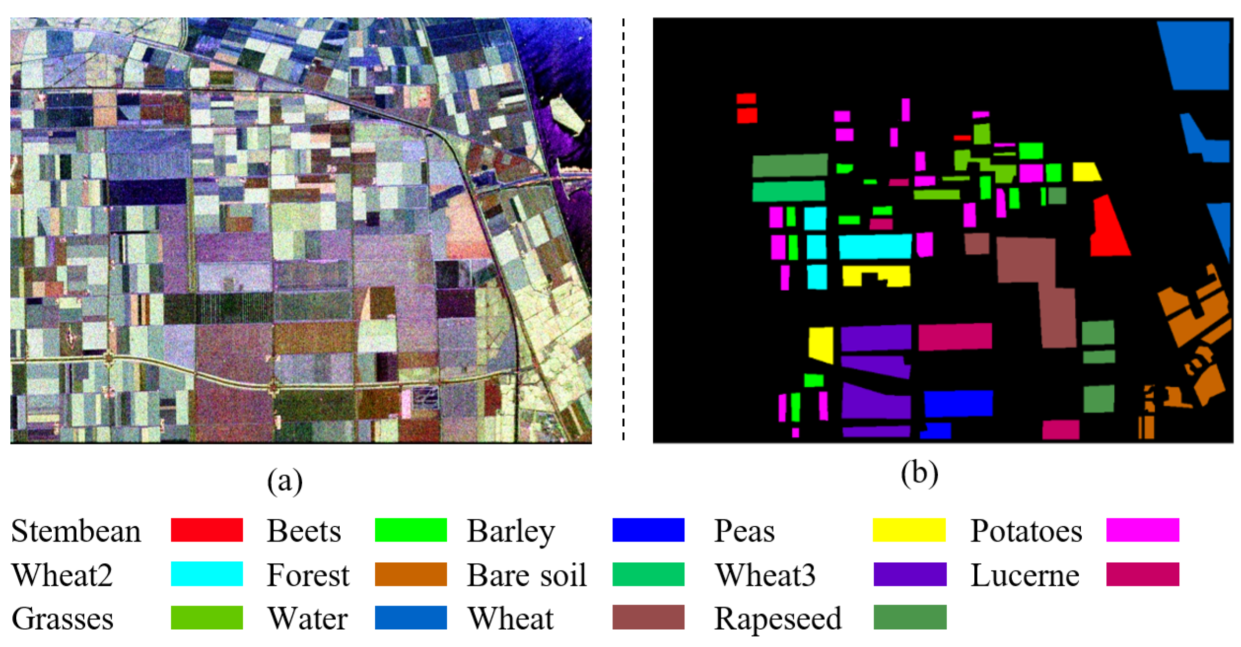
Flevoland full PolSAR data are farmland images at L wave band and were acquired by the AIRSAR Aircraft platform in 16 August 1989. It contains HH, HV, VH and VV (H and V represent horizontal polarization and vertical polarization respectively) channels of polarimetric information. Each channel has 750 × 1024 pixels. The resolution of the image is 6.6 m in the range direction and 12.1 m in the azimuth direction. Since the complex coherent matrix T can describe the scattering mechanism, we transform the 4-channel original data to T. According to Section 3.1, we convert the T in the 6Ch and 4-channel original data to the Pauli RGB image. Figure 4a depicts a Pauli RGB image which includes crops, lake and lands, etc. In this experiment, we first choose 14 types of land cover classes to complete the classification. Then we use the ArcGIS to obtain the ground-truth image of Flevoland according to the Pauli RGB image and google earth. The ground-truth image of Flevoland is shown in Figure 4b.
When we obtain the 6Ch and Pauli RGB image, we can acquire slices as illustrated in Section 3.1.3. In Equation (10), we set s to 15 and i to 5. Then, we obtain slices with the size of 15 × 15. Due to the fact that the images are converted into the 6Ch and 3-channel Pauli RGB image, the numbers of the slices of two branches are and respectively. Subsequently, we label the slices per ground-truth. Finally, we divide the slices into two parts, one is the training set and the other is the testing set. Usually, we chose 75% slices as the training set and the remaining slices as the testing set. It is worth noting that the slices in the same location of the 6Ch and Pauli RGB image should be assigned to an individual part. Table 1 shows the terrain training set and the testing set in the 6Ch and Pauli RGB image; it only includes 14 types of land cover on the ground-truth image.
4.2. Comparing with One-CNN
To verify the effectiveness of the Dual-CNN model, we compare the proposed method with the 6Ch-CNN and PauliRGB-CNN. We apply a Softmax classifier after their own respective last layers. In this way, we can train and test the networks with the same parameters.
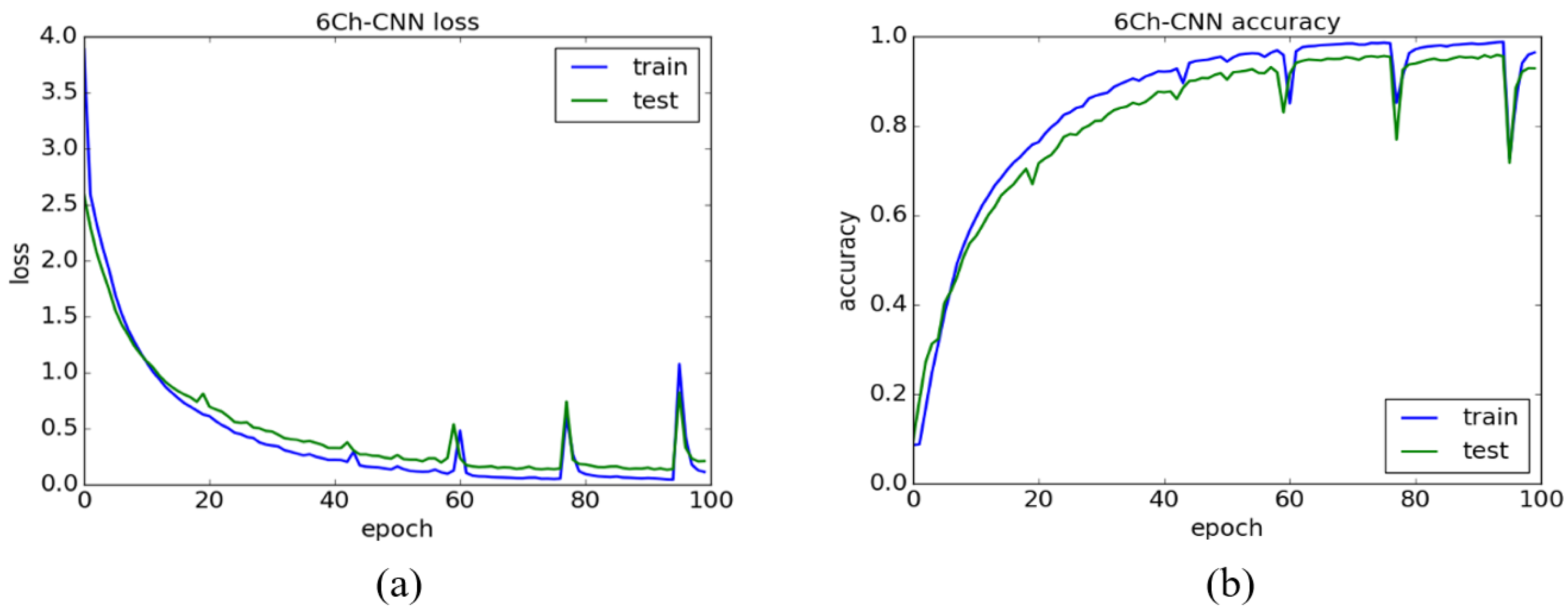
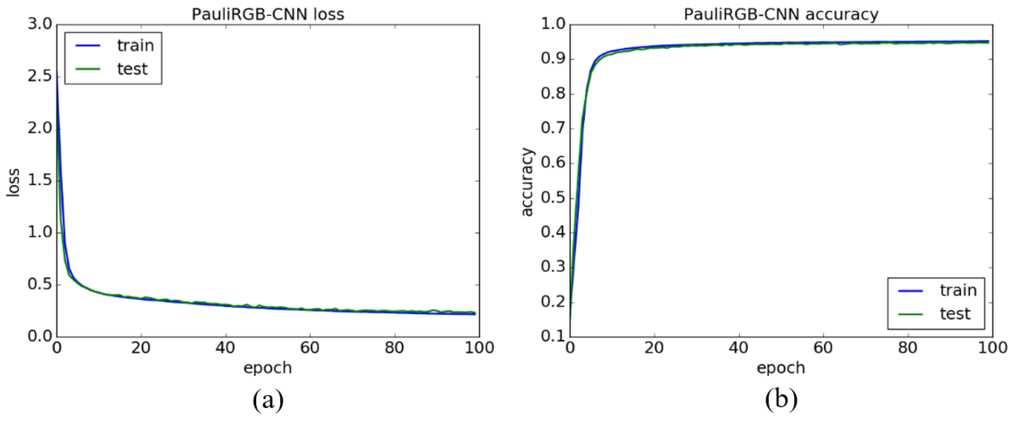
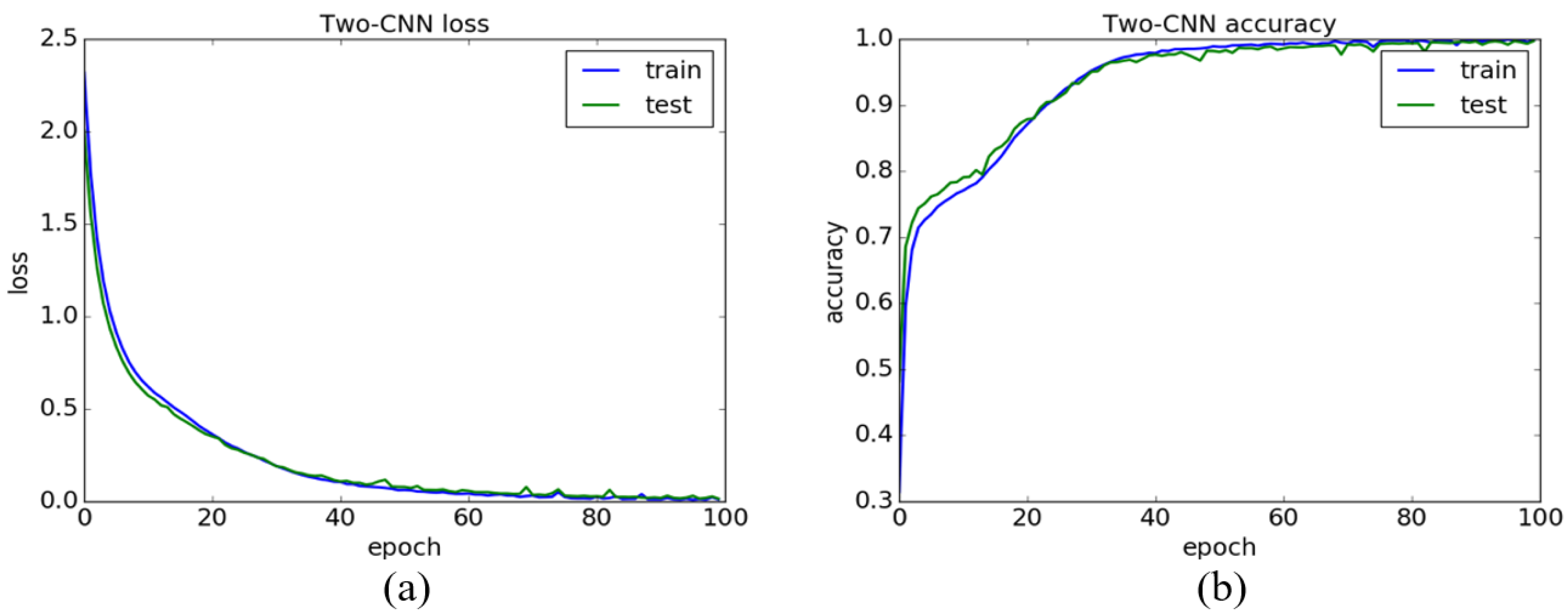
The training process of our method is performed iteratively 100 times on NVIDIA’s GeForce GTX 1070 with 8GB of GPU memory, and 1000 training samples are used in every epoch. Figure 5a, Figure 6a and Figure 7a show the loss curve of the 6Ch-CNN, PauliRGB-CNN and Dual-CNN, where the horizontal axis represents the number of epochs and the vertical axis denotes the loss value. Figure 5b, Figure 6b and Figure 7b show the accuracy curve of the 6Ch-CNN, PauliRGB-CNN and Dual-CNN, where the horizontal axis represents the number of epochs and the vertical axis denotes the classification accuracy. In addition, the blue line depicts the training curve and the green line indicates the testing curve.
As shown in Figure 5, the loss curve of the 6Ch-CNN is not very stable, and its accuracy curve has a large fluctuation as shown in Figure 5b. It is due to the fact that the 6Ch-CNN cannot obtain the general features of the same class in complicated polarimetric data. Moreover, compared with the 6Ch-CNN, although the loss curve and accuracy curve are stable in PauliRGB-CNN, the 3-channel data of the Pauli RGB image are scarce. This fact causes the accuracy rate of the PauliRGB-CNN to be below 95%.
However, in Figure 7b, it can be found that the training accuracy of the Dual-CNN reaches 100%. The testing accuracy is becoming coincident, keeping at 98%. The training loss and the testing loss are stable except for the 45th, 70th and 75th epoch. It proves that the polarimetric features and spatial features are well combined. In Figure 7a, the loss value of the Dual-CNN model decreases, beginning with a minor value 2.25, in which case the training accuracy is 50%, cutting down the training time and the number of epochs. That proved the validity of Equation (13). We draw the conclusion in terms of the accuracy that although there are some anomalies in the training set, the Dual-CNN model is not impacted.
To clarify the result, we list the accuracy rate of the three different methods in Table 2. For the classification of 14 types of land cover classes, the lowest accuracy rate of the Dual-CNN model is still above 95%. Especially, the accuracies of Wheat2 (Label: 6) and Bare soil (Label: 8) reach 100%. However, the average accuracies of the 6Ch-CNN and PauliRGB-CNN are 5.71% and 4.45% lower than the Dual-CNN model.
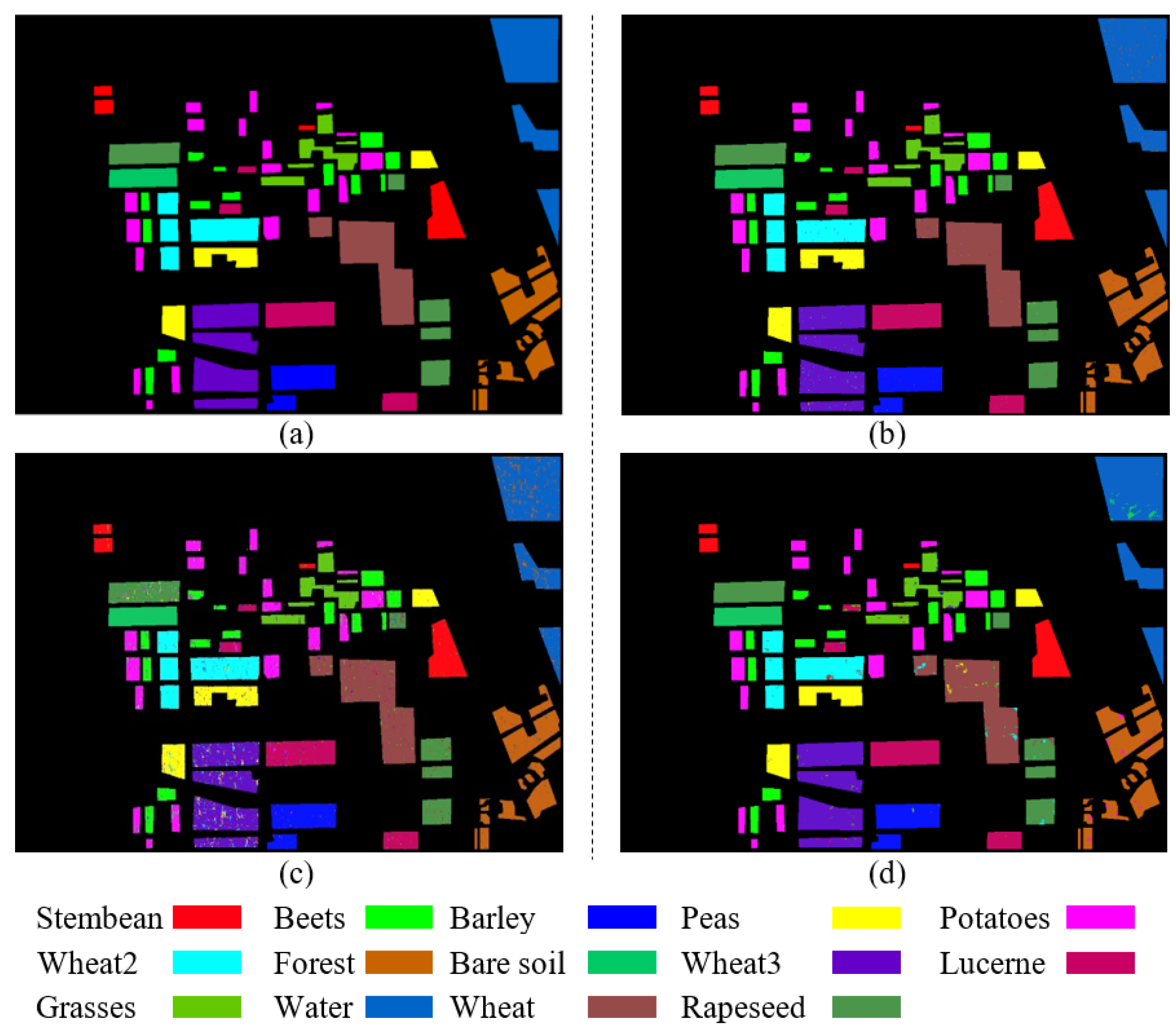
For the convenience of comparison, the classified results are labelled using the same color as the ground-truth. The results of the ground-truth, Dual-CNN, 6Ch-CNN and PauliRGB-CNN are shown in Figure 8a–d, respectively.
Analyzing Figure 8c,d, we find that the 6Ch-CNN and PauliRGB-CNN have obvious faults. The 6Ch-CNN tends to have more scatter errors while PauliRGB-CNN tends to have block errors. However, the Dual-CNN only has a few scatter errors and almost no block errors, which is better than the single branch way. It also demonstrates that the combination of the 6Ch-CNN and PauliRGB-CNN with a fully connected layer is effective for classification.
4.3. Comparing with Other Methods
In this section, we compare our method with some classical algorithms and some newly published methods on the same dataset. The classical algorithms include Maximum Likelihood [18], Support Vector Machine (SVM) [19], and Minimum Distance [20], which are all performed on the ENVI remote sensing image processing platform [21,22]. Lee et al. [23], Zhou et al. [15] and Wang et al. [24] are newly published methods; the method of Lee et al. is an unsupervised algorithm, and those of Zhou et al. and Wang et al. are supervised algorithms.
Table 3 shows the results of the classification. We performed our experiment on both 11 and 14 types of land cover classes. For classical algorithms, SVM has the highest accuracy, but it is still lower than our method. For these newly published methods, supervised algorithms are better than unsupervised ones; the method of Zhou et al. is better than others’ supervised algorithms for 11 classes because of using the CNN. However, our method is still the best. In addition, we find that the accuracy decreases when the number of classes increases.
4.4. Different Fixed Size Slices and Visualization of Feature Maps
4.4.1. The Effect of Slicing Size on Classification Accuracy
The category of the center pixel in the slice served as the label. In order to evaluate how the slice size influences the performance of the algorithm, we performed the experiment with slices of 11 × 11, 15 × 15 and 19 × 19, which are subject to the span equalling to 5. The results of the classification are shown in Figure 9 and Figure 10.
As shown in Figure 9, the experiment which uses the slices of 11 × 11 and 19 × 19 has lower classification accuracy than that of using slices of 15 × 15. Therefore, the slices of 15 × 15 are appropriate for Flevoland full PolSAR data. As is shown in Figure 10a, for the slices of 11 × 11, the Dual-CNN does not perform well for large area targets such as wheat (Wheat: brown; Wheat3: purple); and as is shown in Figure 10b, for the slices of 19 × 19, the Dual-CNN does not perform well for small area targets such as stem bean, peas and so on. However, for the slices of 15 × 15, as shown in Figure 8b, the Dual-CNN conducted on large or small area targets such as wheat or stem beans and peas is better than that of the other two methods. The slice size affects the Dual-CNN classification accuracy.
If the size of the slice is too small, then the Dual-CNN learns inadequate feature information. Slices of large area targets, such as the wheat category, will contain the reduplicated information. Therefore, the features of large area targets learned by the Dual-CNN are not only small in number but also single, which leads to the low classification accuracy. As the size of slices is enlarged, the learning ability of the feature enhances, and the classification accuracy is improved. However, if the size of slices is too large, it will contain the extra features of other objects, which would cause the features of the small area targets to be submerged by other surrounding features. Thus, the Dual-CNN can extract many useless features of small area targets, and the accuracy of classification will decrease.
4.4.2. The Visualization of Feature Maps
To better represent the Dual-CNN model, the 6Ch-CNN and the PauliRGB-CNN are visualized in this paper. As is shown in Figure 11, the visualization processes of two branches are located at the convolution layer and max-pooling layer. The visualization contents include input data visualization, feature extraction visualization, and convolution kernel visualization.
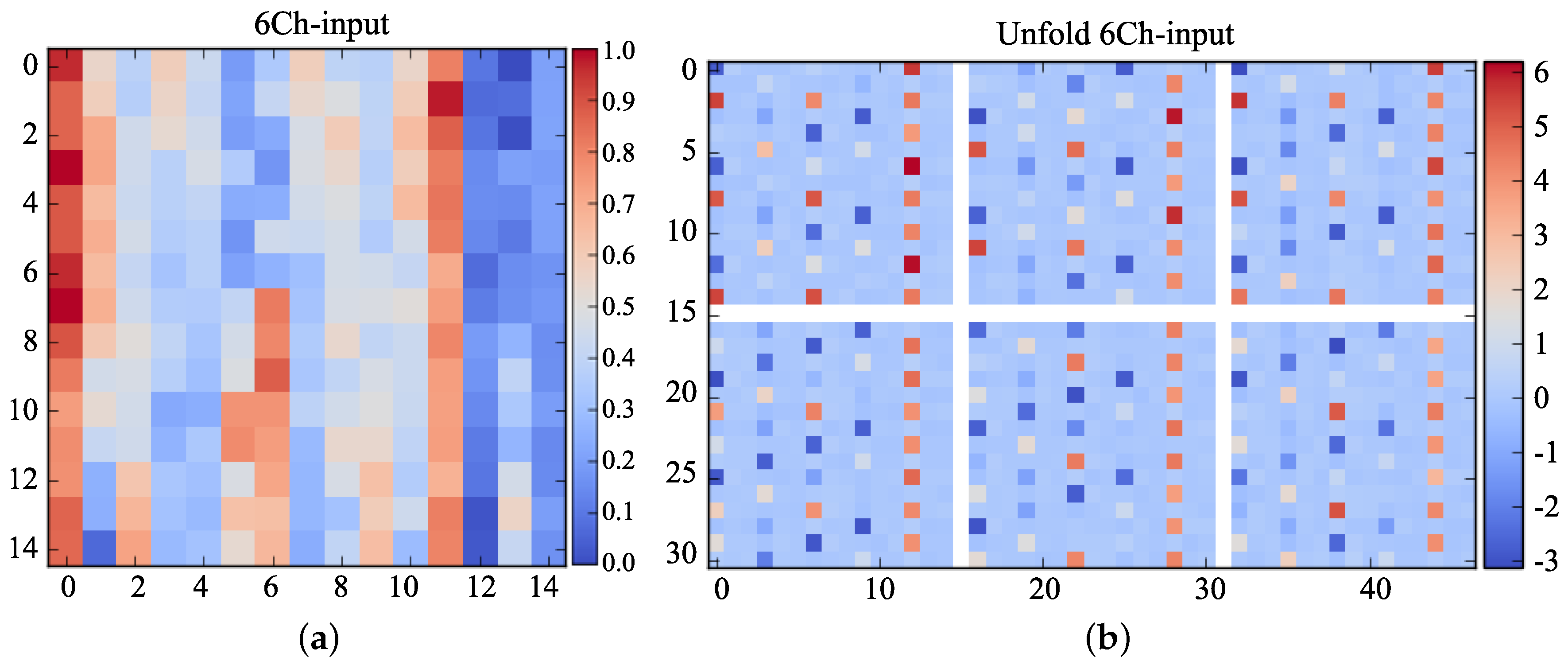
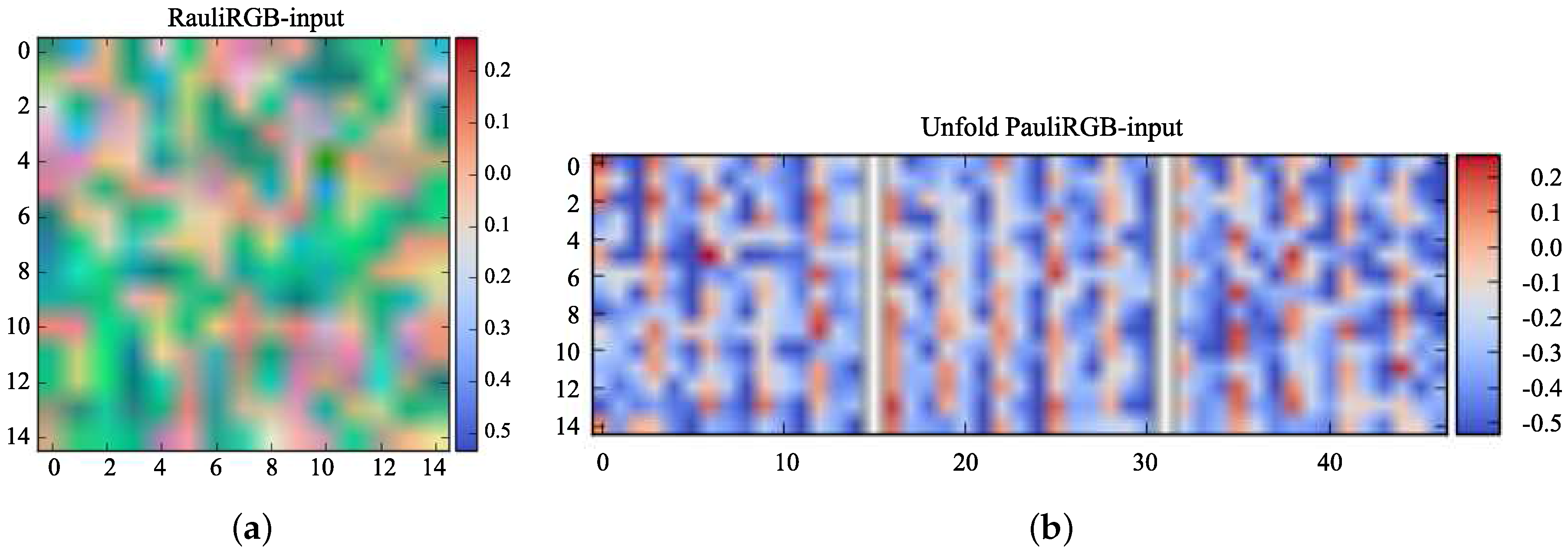
For input data visualization, two Lucerne slices of 15 × 15, which come from the 6Ch and Pauli RGB image in the same location, are selected as the samples to show the visualization process. Two slices are named as the 6Ch-input and PauliRGB-input respectively. Figure 12, Figure 13 and Figure 14 represent the visualization process of the 6Ch-CNN, and Figure 15, Figure 16 and Figure 17 depict the visualization process of the PauliRGB-CNN. Figure 12 and Figure 15 show the visualized images of 6Ch-input and PauliRGB-input; where Figure 12a and Figure 15a denote the mixed visualized images of the 6Ch-input and PaulRGB-input respectively, Figure 12b and Figure 15b denote their unfolded visualized images in an individual channel. Since the data information of the 6Ch-input and PauliRGB-input are significantly different, it is difficult to infer whether they represent the same object from the visualized images. As shown in Figure 12, both the mixed and unfolded visualized images have scatter pixels for the 6Ch-input. This reflects the various scattering phenomena of the polarized waves. In Figure 15, for the PauliRGB-input, some contours can be observed from the mixed and unfolded visualized images. This indicates the spatial characteristics of the terrain surface. These are the most salient features that the CNN requires, which is beneficial for enhancing the classification accuracy. After this visualization process, the 6Ch-input and the PauliRGB-input are put into the trained Dual-CNN model.
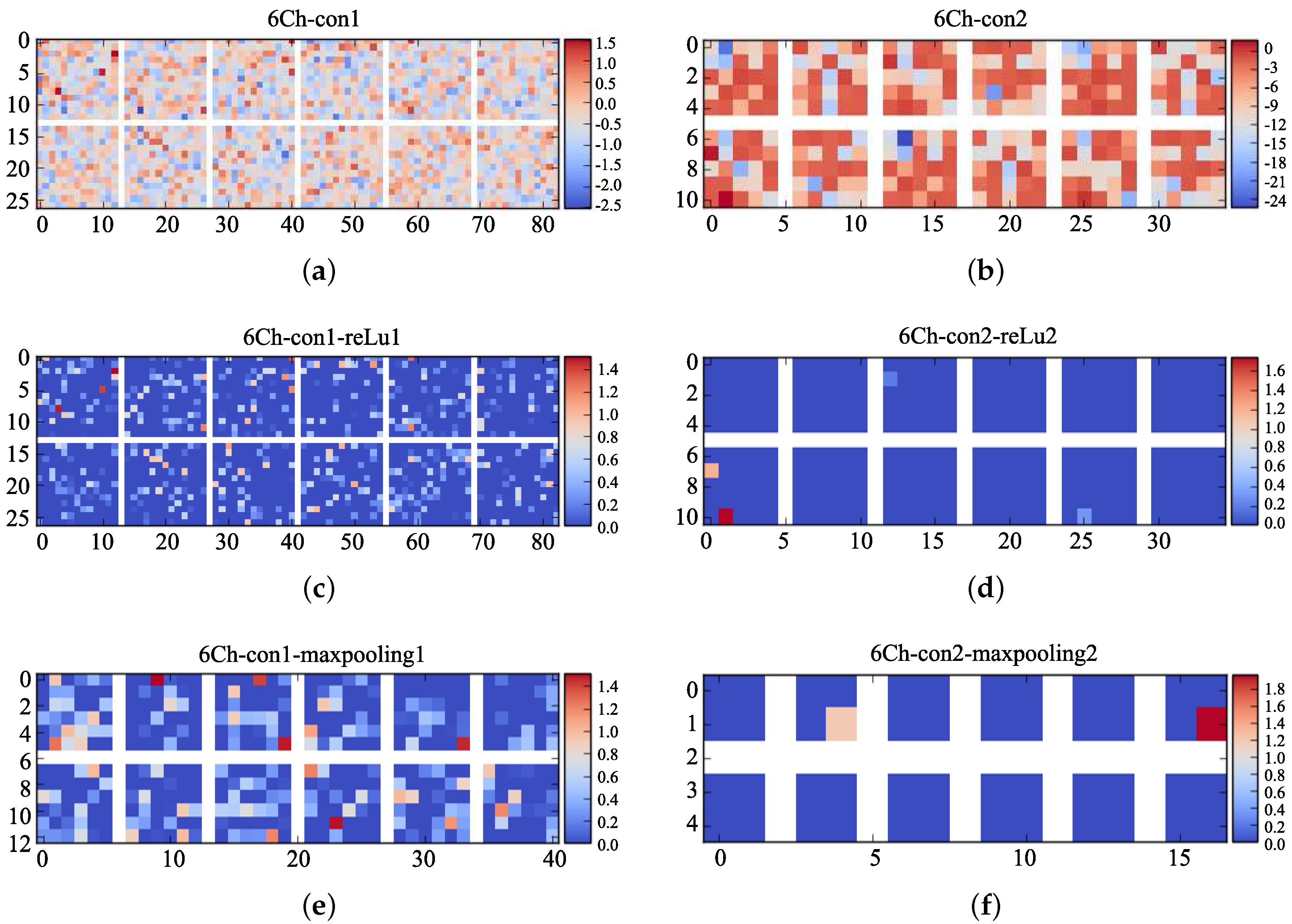
As shown in Figure 1, the feature extraction process is performed with three operations, i.e., convoluting, ReLu processing, and pooling processing. Figure 13 depicts the visualized image of the 6Ch-input during extracting features where Figure 13a–c denote the visualization of the convolution operation, ReLu operation and max-pooling operation of the first round of feature extraction; and Figure 13d–f represent the visualization of the second round of feature extraction. As is shown in Figure 13a, the 15 × 15 6Ch-input serves as the input of the 6Ch-CNN. Then, these data are processed by the 3 × 3 convolution kernel in the first layer and are converted into a 14 × 14 feature map as the output. Figure 13 shows the derived 12 visualized images. Compared with Figure 12b, the salient polarization features are preserved since 0 elements (light orange) in the 6Ch-con1 are increased. Figure 13b illustrates the feature map of the 6Ch-con1-reLu1 after ReLu operation; thus, most of the data are set to 0 (blue). By the max-pooling operation, the visualized feature map of 6Ch-con1-reLu1-maxpooling1 after the first round of feature extraction can be obtained, as shown in Figure 13c. Although the polarization features are salient, there exists a lot of redundancy, so a second round of feature extraction is recommended. The processes are shown in Figure 13d–f. Figure 13f shows the final visualized feature map, where the red squares and the orange squares are the basic features of the input slices.
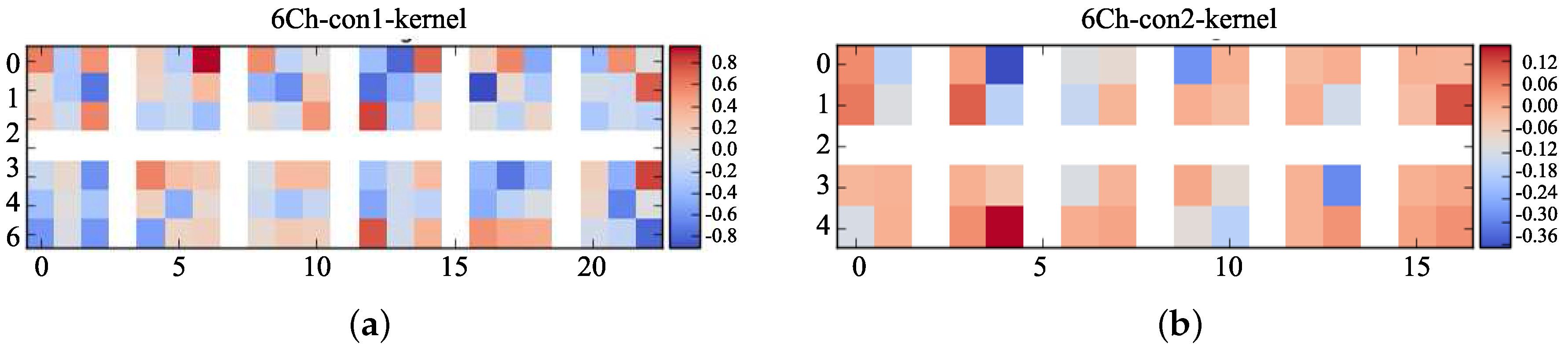
The visualized feature maps of the convolution kernels in the two rounds of feature extraction are shown in Figure 14a,b. From the colorful block in Figure 14, it can be found that the elements of each convolution kernel are not all zero, which indicates that the Dual-CNN has been well trained and the obtained features are obvious.
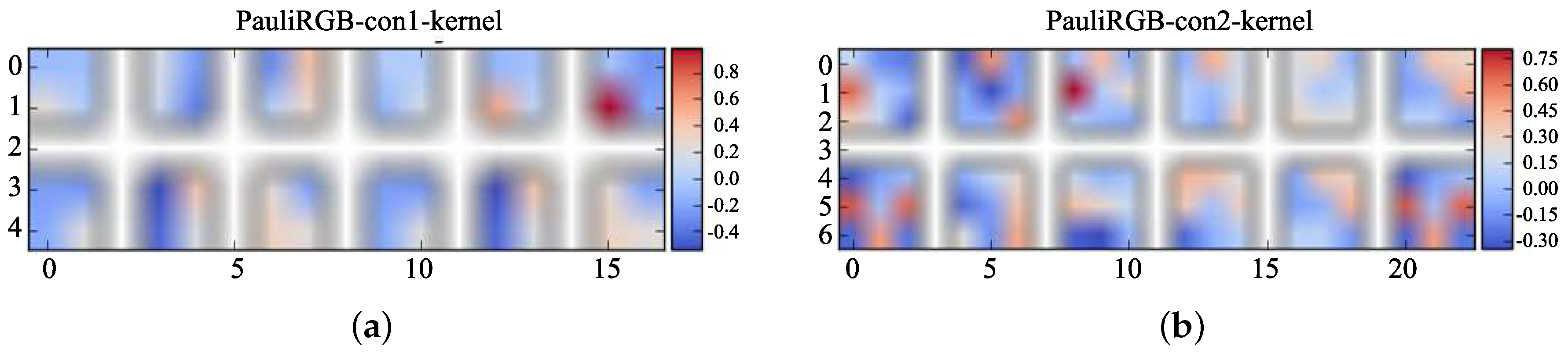
Figure 16 and Figure 17 show the visualization of feature extraction and convolution kernels for the PauliRGB-input. It illustrates that the PauliRGB-input requires a second round of feature extraction to extract more abstract spatial features as done in the 6Ch-input.
Note that the features extracted by the 6Ch-CNN and PauliRGB-CNN have polarimetric and spatial characteristics. Visualization can help to check whether the Dual-CNN model is well trained and to illustrate how to extract the P-S features.
5. Conclusions
By exploring the unique characteristics of the PolSAR data, we have presented a new method that achieves excellent accuracy in PolSAR classification. The main contributions of this work lie in the following three aspects. First, we proposed a method of pre-processing the PolSAR data to facilitate subsequent work. Second, a novel CNN framework which consists of two CNNs was presented to extract and fuse the polarization feature and spatial feature of the pre-processed data. Last but not least, visualization of the CNN was applied to help us tune the parameters of the model. We carried out the experiments on 14 types of land cover classes, and the results show that our model is superior to the classical classification methods such as SVM, and Maximum Likelihood. Compared with a single CNN, our method still has higher accuracy due to its P-S features.
Acknowledgments
This work was supported by the National Natural Science Foundation of China (61071139; 61471019; 61671035), the Aeronautical Science Foundation of China (20142051022), the Pilot Project (9140A07040515HK01009), the Scientific Research Foundation of Guangxi Education Department (KY 2015LX443), and the Scientific Research and Technology Development Project of Wuzhou City, GuangXi, China (201402205).
Author Contributions
Fei Gao and Teng Huang conceived of and designed the experiments. Jun Wang performed the experiments. Jinping Sun, Amir Hussain, Erfu Yang analyzed the data and wrote the paper.
Conflicts of Interest
The authors declare no conflict of interest.
References
- Gaber, A.; Soliman, F.; Koch, M.; El-Baz, F. Using full-polarimetric SAR data to characterize the surface sediments in desert areas: A case study in El-Gallaba Plain, Egypt. Remote Sens. Environ. 2015, 162, 11–28. [Google Scholar] [CrossRef]
- Canty, M.J. Images, Arrays, and Matrices. In Image Analysis, Classification and Change Detection in Remote Sensing: With Algorithms for ENVI/IDL and Python, 3rd ed.; CRC Press: Boca Raton, FL, USA, 2014; pp. 1–32. [Google Scholar]
- Rosenqvist, A.; Shimada, M.; Ito, N.; Watanabe, M. ALOS PALSAR: A Pathfinder mission for global-scale monitoring of the environment. IEEE Trans. Geosci. Remote Sens. 2007, 45, 3307–3316. [Google Scholar] [CrossRef]
- Yang, M.; Zhang, G. A novel ship detection method for SAR images based on nonlinear diffusion filtering and Gaussian curvature. Remote Sens. Lett. 2016, 7, 211–219. [Google Scholar] [CrossRef]
- Niu, C.; Zhang, G.; Zhu, J.; Liu, S.; Ma, D. Correlation Coefficients Between Polarization Signatures for Evaluating Polarimetric Information Preservation. IEEE Geosci. Remote Sens. Lett. 2011, 8, 1016–1020. [Google Scholar] [CrossRef]
- Deng, L.; Yan, Y.N.; Sun, C. Use of Sub-Aperture Decomposition for Supervised PolSAR Classification in Urban Area. Remote Sens. 2011, 7, 1380–1396. [Google Scholar] [CrossRef]
- Xiang, D.L.; Tang, T.; Hu, C.B.; Fan, Q.H.; Su, Y. Built-up Area Extraction from PolSAR Imagery with Model-Based Decomposition and Polarimetric Coherence. Remote Sens. 2016, 8, 685. [Google Scholar] [CrossRef]
- Hinton, G.E.; Salakhutdinov, R.R. Reducing the dimensionality of data with neural networks. Science 2006, 313, 504–507. [Google Scholar] [CrossRef] [PubMed]
- Wong, W.K.; Sun, M. Deep Learning Regularized Fisher Mappings. IEEE Trans. Neural Netw. 2011, 22, 1668–1675. [Google Scholar] [CrossRef] [PubMed]
- Han, J.; Zhang, D.; Cheng, G.; Guo, L.; Ren, J. Object Detection in Optical Remote Sensing Images Based on Weakly Supervised Learning and High-Level Feature Learning. IEEE Trans. Geosci. Remote Sens. 2015, 53, 3325–3337. [Google Scholar] [CrossRef]
- Vincent, P.; Larochelle, H.; Lajoie, I.; Bengio, Y.; Manzagol, P.A. Stacked denoising autoencoders: Learning useful representations in a deep network with a local denoising criterion. J. Mach. Learn. Res. 2010, 11, 3371–3408. [Google Scholar]
- Sun, M.J.; Zhang, D.; Ren, J.C.; Wang, Z.; Jin, J.S. Brushstroke Based Sparse Hybrid Convolutional Neural Networks for Author Classification of Chinese Ink-Wash Paintings. In Proceedings of the 2015 IEEE International Conference on Image Processing (ICIP), Quebec City, QC, Canada, 27–30 September 2015; pp. 626–630. [Google Scholar]
- Krizhevsky, A.; Sutskever, I.; Hinton, G.E. ImageNet classification with deep convolutional neural networks. Adv. Neural Inf. Proc. Syst. 2012, 25, 1097–1105. [Google Scholar]
- Wang, Y.Y.; Wang, G.H.; Lan, Y.H. PolSAR Image Classification Based on Deep Convolutional Neural Network. Metall. Min. Ind. 2015, 8, 366–371. [Google Scholar]
- Zhou, Y.; Wang, H.P.; Xu, F.; Jin, Y.Q. Polarimetric SAR Image Classification Using Deep Convolutional Neural Networks. IEEE Geosci. Remote Sens. Lett. 2016, 99, 1–5. [Google Scholar] [CrossRef]
- Aghababaee, H.; Amini, J. Contextual PolSAR image classification using fractal dimension and support vector machines. Eur. J. Remote Sens. 2013, 46, 317–332. [Google Scholar] [CrossRef]
- Margarit, G.; Mallorqui, J.J.; Fabregas, X. Single-Pass Polarimetric SAR Interferometry for Vessel Classification. Geosci. Remote Sens. IEEE Trans. 2007, 45, 3494–3502. [Google Scholar] [CrossRef]
- Bruzzone, L.; Prieto, D.F. Unsupervised retraining of a maximum likelihood classifier for the analysis of multitemporal remote sensing images. IEEE Trans. Geosci. Remote Sens. 2001, 39, 456–460. [Google Scholar] [CrossRef]
- Zhao, Q.; Principe, J.C. Support vector machines for SAR automatic target recognition. IEEE Trans. Aerosp. Electron. Syst. 2001, 37, 643–654. [Google Scholar] [CrossRef]
- Zhang, D.; Chen, S.; Zhou, Z.H. Rapid and brief communication: Learning the kernel parameters in kernel minimum distance classifier. Pattern Recognit. 2006, 39, 133–135. [Google Scholar] [CrossRef]
- Wang, Y.P.; Chen, D.F.; Song, Z.G. Detecting surface oil slick related to gas hydrate/petroleum on the ocean bed of South China Sea by ENVI/ASAR radar data. J. Asian Earth Sci. 2013, 65, 21–26. [Google Scholar] [CrossRef]
- Aplin, P. Image Analysis, Classification and Change Detection in Remote Sensing, with algorithms for ENVI/IDL. Int. J. Geogr. Inf. Sci. 2009, 23, 129–130. [Google Scholar]
- Lee, J.S.; Grunes, M.R.; Pottier, E. Quantitative comparison of classification capability: Fully polarimetric versus dual and single-polarization SAR. IEEE Trans. Geosci. Remote Sens. 2001, 39, 2343–2351. [Google Scholar]
- Wang, H.; Zhou, Z.; Turnbull, J.; Song, Q.; Qi, F. Pol-SAR classification based on generalized polar decomposition of mueller matrix. IEEE Trans. Geosci. Remote Sens. 2016, 13, 565–569. [Google Scholar] [CrossRef]
Figure 1.
The processing of feature extraction in deep convolution neural network (CNN).

Figure 2.
The main procedures of the polarimetric synthetic aperture radar (PolSAR) images classification based on the dual-branch deep convolution neural network (Dual-CNN) model.
Figure 2.
The main procedures of the polarimetric synthetic aperture radar (PolSAR) images classification based on the dual-branch deep convolution neural network (Dual-CNN) model.

Figure 3.
The generation of the fixed-size slices based on the center pixel.

Figure 4.
(a) Pauli RGB image of Flevoland PolSAR data; (b) Ground-truth image of Flevoland.

Figure 5.
(a) Loss curve of the 6Ch-CNN; (b) accuracy curve of the 6Ch-CNN.

Figure 6.
(a) Loss curve of the PauliRGB-CNN; (b) accuracy curve of the PauliRGB-CNN.

Figure 7.
(a) Loss curve of the Dual-CNN; (b) accuracy curve of the Dual-CNN.

Figure 8.
(a–d) represent the classification results of the ground-truth, Dual-CNN, 6Ch-CNN, and PauliRGB-CNN, respectively.
Figure 8.
(a–d) represent the classification results of the ground-truth, Dual-CNN, 6Ch-CNN, and PauliRGB-CNN, respectively.

Figure 9.
The classification accuracy of the Dual-CNN with the slices of different sizes.

Figure 10.
(a,c) represent the classification results of the Dual-CNN with slices of 11 × 11 and 19 × 19 respectively; (b,d) display the false results in (a,c).
Figure 10.
(a,c) represent the classification results of the Dual-CNN with slices of 11 × 11 and 19 × 19 respectively; (b,d) display the false results in (a,c).

Figure 11.
The location of the visualization process.

Figure 12.
(a) Mixed visualized image of the 6Ch-input; (b) Unfolded visualized images of the 6Ch-input.
Figure 12.
(a) Mixed visualized image of the 6Ch-input; (b) Unfolded visualized images of the 6Ch-input.

Figure 13.
Visualized feature maps of the 6Ch-input. (a,c,e) denote the visualized feature maps of the convolution operation, ReLu operation and max-pooling operation in the first round of feature extraction; and (b,d,f) denote the visualization of the second round of feature extraction.
Figure 13.
Visualized feature maps of the 6Ch-input. (a,c,e) denote the visualized feature maps of the convolution operation, ReLu operation and max-pooling operation in the first round of feature extraction; and (b,d,f) denote the visualization of the second round of feature extraction.

Figure 14.
Visualization of the convolution kernel of the 6Ch-CNN: (a) visualization of the convolution kernel in the first round of feature extraction; and (b) visualization of the convolution kernel in the second round of feature extraction.
Figure 14.
Visualization of the convolution kernel of the 6Ch-CNN: (a) visualization of the convolution kernel in the first round of feature extraction; and (b) visualization of the convolution kernel in the second round of feature extraction.

Figure 15.
(a) Mixed visualized image of the PauliRGB-input; (b) Unfolded visualized images of the PauliRGB-input.
Figure 15.
(a) Mixed visualized image of the PauliRGB-input; (b) Unfolded visualized images of the PauliRGB-input.

Figure 16.
Visualized feature maps of the PauliRGB-input. (a,c,e) denote the visualized feature maps of the convolution operation, ReLu operation and max-pooling operation in the first round of feature extraction; (b,d,f) denote the visualization in the second round of feature extraction.
Figure 16.
Visualized feature maps of the PauliRGB-input. (a,c,e) denote the visualized feature maps of the convolution operation, ReLu operation and max-pooling operation in the first round of feature extraction; (b,d,f) denote the visualization in the second round of feature extraction.

Figure 17.
Visualization of the convolution kernel of the PauliRGB-CNN: (a) visualization of the convolution kernel in the first round of feature extraction; and (b) visualization of the convolution kernel in the second round of feature extraction.
Figure 17.
Visualization of the convolution kernel of the PauliRGB-CNN: (a) visualization of the convolution kernel in the first round of feature extraction; and (b) visualization of the convolution kernel in the second round of feature extraction.


Table 1.
The detailed information of the training set and testing set on 14 types of land cover classes on Flevoland PolSAR data.
Table 1.
The detailed information of the training set and testing set on 14 types of land cover classes on Flevoland PolSAR data.
| Label | Type | Color | Train | Test | ||
|---|---|---|---|---|---|---|
| 6Ch | PauliRGB | 6Ch | PauliRGB | |||
| 1 | Stembeans | 5082 | 5082 | 1693 | 1693 | |
| 2 | Beets | 6039 | 6039 | 2012 | 2012 | |
| 3 | Barley | 5106 | 5106 | 1701 | 1701 | |
| 4 | Peas | 5530 | 5530 | 1843 | 1843 | |
| 5 | Potatoes | 9180 | 9180 | 3060 | 3060 | |
| 6 | Wheat2 | 7343 | 7343 | 2447 | 2447 | |
| 7 | Forest | 10,093 | 10,093 | 3364 | 3364 | |
| 8 | Bare soil | 3299 | 3299 | 4099 | 4099 | |
| 9 | Wheat3 | 12,663 | 12,663 | 4221 | 4221 | |
| 10 | Lucerne | 6872 | 6872 | 2290 | 2290 | |
| 11 | Grasses | 4200 | 4200 | 1399 | 1399 | |
| 12 | Water | 14,739 | 14,739 | 4913 | 4913 | |
| 13 | Wheat | 12,361 | 12,361 | 4120 | 4120 | |
| 14 | Rapeseed | 9013 | 9013 | 2838 | 2838 | |
| Total | – | – | 111,520 | 111,520 | 37,000 | 37,000 |
Table 2.
The detailed classification accuracy of the Dual-CNN, 6Ch-CNN, and PauliRGB-CNN on Flevoland PolSAR data.
Table 2.
The detailed classification accuracy of the Dual-CNN, 6Ch-CNN, and PauliRGB-CNN on Flevoland PolSAR data.
| Label | Dual-CNN (%) | 6Ch-CNN (%) | PauliRGB-CNN (%) |
|---|---|---|---|
| 1 | 97.77 | 96.04 | 95.64 |
| 2 | 98.21 | 90.85 | 90.70 |
| 3 | 97.88 | 93.94 | 94.17 |
| 4 | 96.72 | 91.91 | 93.67 |
| 5 | 95.96 | 88.56 | 92.57 |
| 6 | 100 | 95.05 | 94.26 |
| 7 | 99.94 | 97.08 | 95.97 |
| 8 | 100 | 95.54 | 93.45 |
| 9 | 95.95 | 87.84 | 90.48 |
| 10 | 99.51 | 92.70 | 94.07 |
| 11 | 98.85 | 95.40 | 95.42 |
| 12 | 99.92 | 91.34 | 96.74 |
| 13 | 99.85 | 93.20 | 93.48 |
| 14 | 99.39 | 90.45 | 95.53 |
| overall | 98.56 | 92.85 | 94.01 |
© 2017 by the authors. Licensee MDPI, Basel, Switzerland. This article is an open access article distributed under the terms and conditions of the Creative Commons Attribution (CC BY) license (http://creativecommons.org/licenses/by/4.0/).
Share and Cite
MDPI and ACS Style
Gao, F.; Huang, T.; Wang, J.; Sun, J.; Hussain, A.; Yang, E. Dual-Branch Deep Convolution Neural Network for Polarimetric SAR Image Classification. Appl. Sci. 2017, 7, 447. https://0-doi-org.brum.beds.ac.uk/10.3390/app7050447
AMA Style
Gao F, Huang T, Wang J, Sun J, Hussain A, Yang E. Dual-Branch Deep Convolution Neural Network for Polarimetric SAR Image Classification. Applied Sciences. 2017; 7(5):447. https://0-doi-org.brum.beds.ac.uk/10.3390/app7050447
Chicago/Turabian StyleGao, Fei, Teng Huang, Jun Wang, Jinping Sun, Amir Hussain, and Erfu Yang. 2017. "Dual-Branch Deep Convolution Neural Network for Polarimetric SAR Image Classification" Applied Sciences 7, no. 5: 447. https://0-doi-org.brum.beds.ac.uk/10.3390/app7050447
Note that from the first issue of 2016, this journal uses article numbers instead of page numbers. See further details here.