Adaptive Intelligent Sliding Mode Control of a Photovoltaic Grid-Connected Inverter

Abstract

Adaptive intelligent sliding mode control methods are developed for a single-phase photovoltaic (PV) grid-connected transformerless system with a boost chopper and a DC-AC inverter. A maximum power point tracking (MPPT) method is implemented in the boost part in order to extract the maximum power from the PV array. A global fast terminal sliding control (GFTSMC) strategy is developed for an H-bridge inverter to make the tracking error between a grid reference voltage and the output voltage of the inverter converge to zero in a finite time. A fuzzy-neural-network (FNN) is used to estimate the system uncertainties. Intelligent methods, such as an adaptive fuzzy integral sliding controller and a fuzzy approximator, are employed to control the DC-AC inverter and approach the upper bound of the system nonlinearities, achieving reliable grid-connection, small voltage tracking error, and strong robustness to environmental variations. Simulation with a grid-connected PV inverter model is implemented to validate the effectiveness of the proposed methods.

1. Introduction

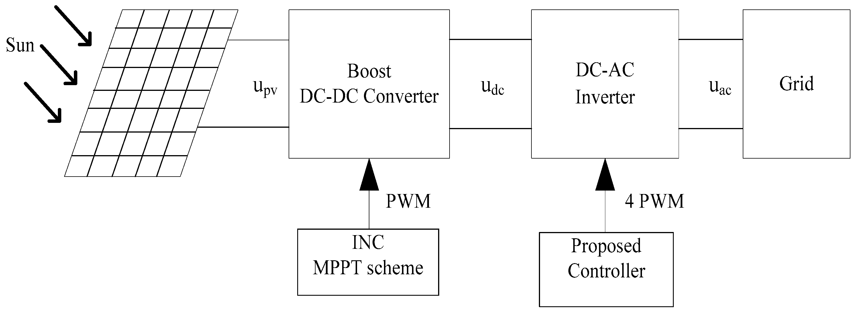
Photovoltaic (PV) generation is attracting significant interests since it is a clean renewable energy. An inverter is indispensable in a PV generation system; therefore, it is necessary to convert PV power into AC power. The advantages of a grid-connected transformerless inverter are its light weight, small size, and low price. A two-stage single-phase PV grid-connected inverter mainly includes a boost chopper and DC-AC converter, where boost and maximum power point tracking (MPPT) are implemented in the boost part, while the conversion from DC to AC is accomplished in the DC-AC converter.

Some MPPT methods [1,2,3,4,5,6], such as constant voltage tracking (CVT), incremental conductance (INC) method, intelligent method, and particle swarm optimization, are developed to track the MPPT to increase the efficiency of the PV inverter. Intelligent methods are utilized to control the PV inverter and active power filter [7,8,9,10,11]. Some scholars have employed sliding mode control (SMC) to control the PV grid-connected inverter. A novel robust adaptive sliding-mode controller for a grid-connected PV inverter was proposed in Reference [12]. Backstepping sliding control and fuzzy sliding control were investigated in References [13,14,15,16,17,18,19] to improve the performance of PV inverters and dynamic systems. An adaptive fuzzy controller and a neural network controller have been developed for a PV grid-connected inverter in References [20,21,22]. Motivated by the above discussion, an adaptive intelligent sliding control is proposed for a PV inverter, and an MPPT algorithm is presented by using an INC method with an adaptive step size. An adaptive fuzzy sliding mode control (AFSMC) method is developed to control the inverter. An adaptive fuzzy neural network global fast terminal sliding mode control (FNNGFTSMC) strategy is utilized for the DC-AC converter. A global fast terminal sliding surface and controller are designed to make the output voltage’s tracking error in the inverter converge to zero in finite time. A FNN whose weights are updated in real time is employed to approximate and adapt the system uncertainties.

The structure of the paper is arranged as follows. The system description of the PV inverter is introduced in Section 2. In Section 3, the MPPT algorithm is introduced. The AFSMC and GFTSMC are proposed in Section 4 and Section 5, respectively. Simulation studies and the discussion are given in Section 6 and the final section gives the conclusions.

2. System Description

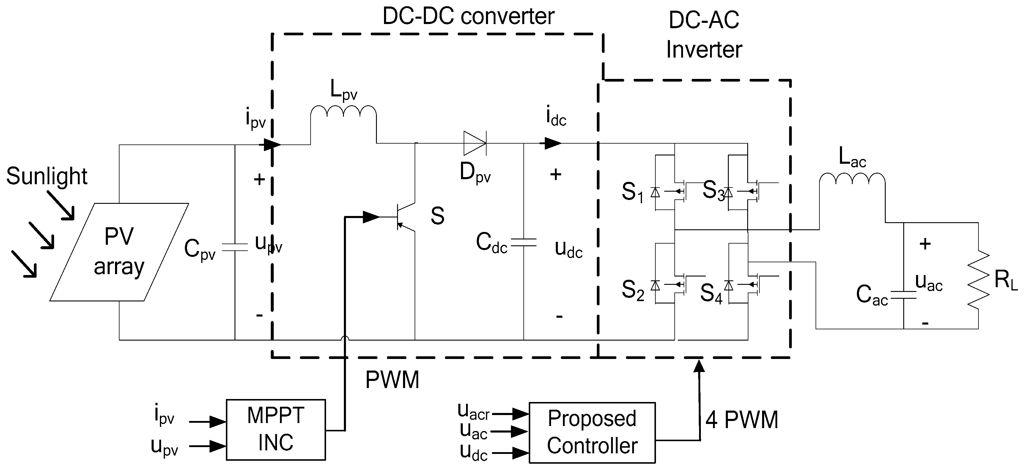
Figure 1 is a typical two-stage single-phase grid-connected PV inverter without an isolation transformer mainly including a boost converter and a DC-AC inverter. The DC-AC inverter is connected to the grid, and it is required that its output voltage is consistent with the reference voltage of the grid.

The following paragraphs describe the model of the two parts.

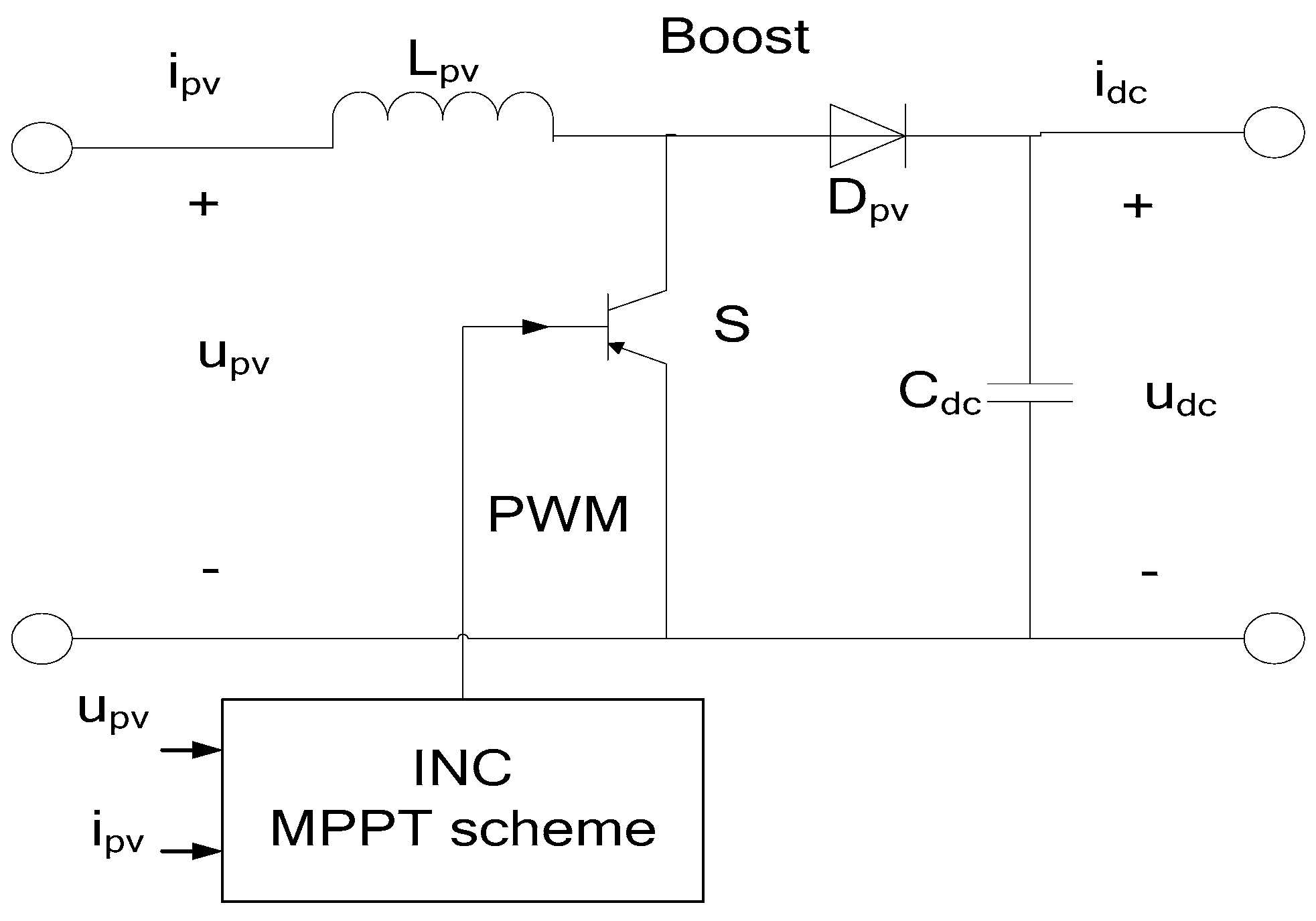
2.1. Boost Model

Figure 2 is the schematic diagram of a boost chopper, where $u_{pv}$ and $i_{pv}$ are the output voltage and current of the PV array respectively. The boost converter is composed of switch $S$, inductance $L_{pv}$, and capacitance $C_{dc}$, together with diode $D_{pv}$.

Assumption 1.

The inductance$L_{pv}$and capacitance$C_{dc}$of the converter are large enough that the current$i_{pv}$and voltage$u_{dc}$keep constant during the switch S on and off time.

It is assumed that the conduction duty cycle of S is $D_b$. Since the energy accumulated by the inductor in one cycle is equal to its released energy, we obtain:

$$u_{pv}{i}_{pv}{D}_b=(u_{dc}-u_{pv})i_{pv}(1-D_b)$$

(1)

The relation $u_{pv}=(1-D_b)u_{dc}$ can be derived from (1).

Actually, $L_{pv}$ and $C_{dc}$ of the converter are finite, and $u_{dc}$ may decrease somewhat. However, when $L_{pv}$ and $C_{dc}$ is large enough, the error can be ignored.

If $0\le D_b\le 1$, then $u_{dc}>u_{pv}$, proving the characteristic of the voltage boosting in the boost chopper. Moreover, $u_{pv}$ and $D_b$ vary inversely when $u_{dc}$ keeps constant. A suitable PV voltage can be obtained by adjusting $D_b$ such that the PV inverter can work at the stage of the maximum power point.

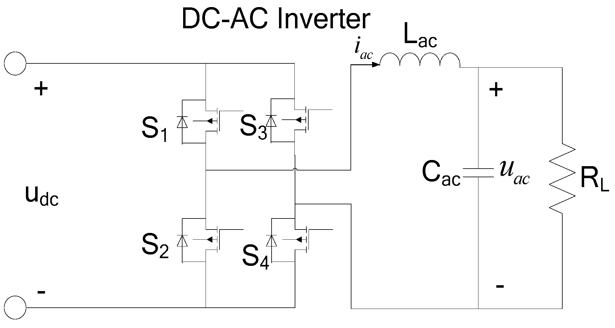
2.2. DC-AC Inverter Model

The DC power is transferred to the grid through the DC-AC inverter. As shown in Figure 3, the DC-AC inverter is composed of four power switches. $S_1-S_4$ are all fully-controlled power switches, and $C_{ac}$ and $L_{ac}$ are the filter capacitance and inductance in the grid side, respectively, $R_L$ is the load.

Some ideal conditions are assumed to derive the dynamic model of the inverter.

Assumption 2.

S₁–S₄ are all ideal switches with zero turn-on impedance, no dead time, and no capacitive or inductance effects. There is no parasitic resistance existing on inductance$L_{ac}$and capacitance$C_{ac}$. There is only one group of switches on at any time, and the opening time and shutdown time for each switch can be ignored since it is small enough.

According to Kirchoff’s Current Law (KCL) and Kirchoff’s Voltage Law (KVL), it can be obtained that:

While S₁, S₄ are on:

$$\{\begin{array}{l}-u_{dc}+L_{ac}\frac{d{i}_{ac}}{dt}+u_{ac}=0\hfill \\ i_{ac}-\frac{1}{R_L}{u}_{ac}-C_{ac}\frac{d{u}_{ac}}{dt}=0\hfill \end{array}$$

(2)

While S₂, S₃ are on:

$$\{\begin{array}{l}{L}_{ac}\frac{d{i}_{ac}}{dt}+u_{dc}+u_{ac}=0\hfill \\ -i_{ac}+C_{ac}\frac{d{u}_{ac}}{dt}+\frac{1}{R_L}{u}_{ac}=0\hfill \end{array}$$

(3)

Assuming that D is the duty cycle of $S_1$ and $S_4$, then the duty cycle of S₂ and S₃ is one dimensional. According to the state space average model, the mathematical expression of the inverter can be expressed as:

$$\{\begin{array}{l}{L}_{ac}\frac{d{i}_{ac}}{dt}=(2D-1)u_{dc}-u_{ac}\hfill \\ C_{ac}\frac{d{u}_{ac}}{dt}=i_{ac}-\frac{1}{R_L}{u}_{ac}\hfill \end{array}$$

(4)

Then, the derivative equation is obtained as:

$$\frac{d^2{u}_{ac}}{d{t}^2}=-\frac{1}{R_L{C}_{ac}}\frac{d{u}_{ac}}{dt}-\frac{1}{L_{ac}{C}_{ac}}{u}_{ac}+\frac{2D-1}{L_{ac}{C}_{ac}}{u}_{dc}$$

(5)

In practical applications, parameter variations and external disturbances always have an influence on the inverter. Considering the uncertainties in the inverter, Equation (5) can be rewritten as:

$$\frac{d^2{u}_{ac}}{d{t}^2}=-(\frac{1}{R_L{C}_{ac}}+{\Delta }_1)\frac{d{u}_{ac}}{dt}-(\frac{1}{L_{ac}{C}_{ac}}+{\Delta }_2)u_{ac}+(\frac{2D-1}{L_{ac}{C}_{ac}}+{\Delta }_3)u_{dc}+d(t)$$

(6)

where the parameter variations are ${\Delta }_1$, ${\Delta }_2$, and ${\Delta }_3$, and external disturbances are $d(t)$, which result from the instability of $u_{dc}$. Let $g(t)=-{\Delta }_1\frac{d{u}_{ac}}{dt}-{\Delta }_2{u}_{ac}+{\Delta }_3{u}_{dc}+d(t)$, and the dynamic model of the inverter is obtained as Equation (7):

$$\frac{d^2{u}_{ac}}{d{t}^2}=-\frac{1}{R_L{C}_{ac}}\frac{d{u}_{ac}}{dt}-\frac{1}{L_{ac}{C}_{ac}}{u}_{ac}+\frac{2D-1}{L_{ac}{C}_{ac}}{u}_{dc}+g(t)$$

(7)

where $u_{ac}$ and its derivative, as well as $u_{dc}$, can be measured.

3. MPPT Approach

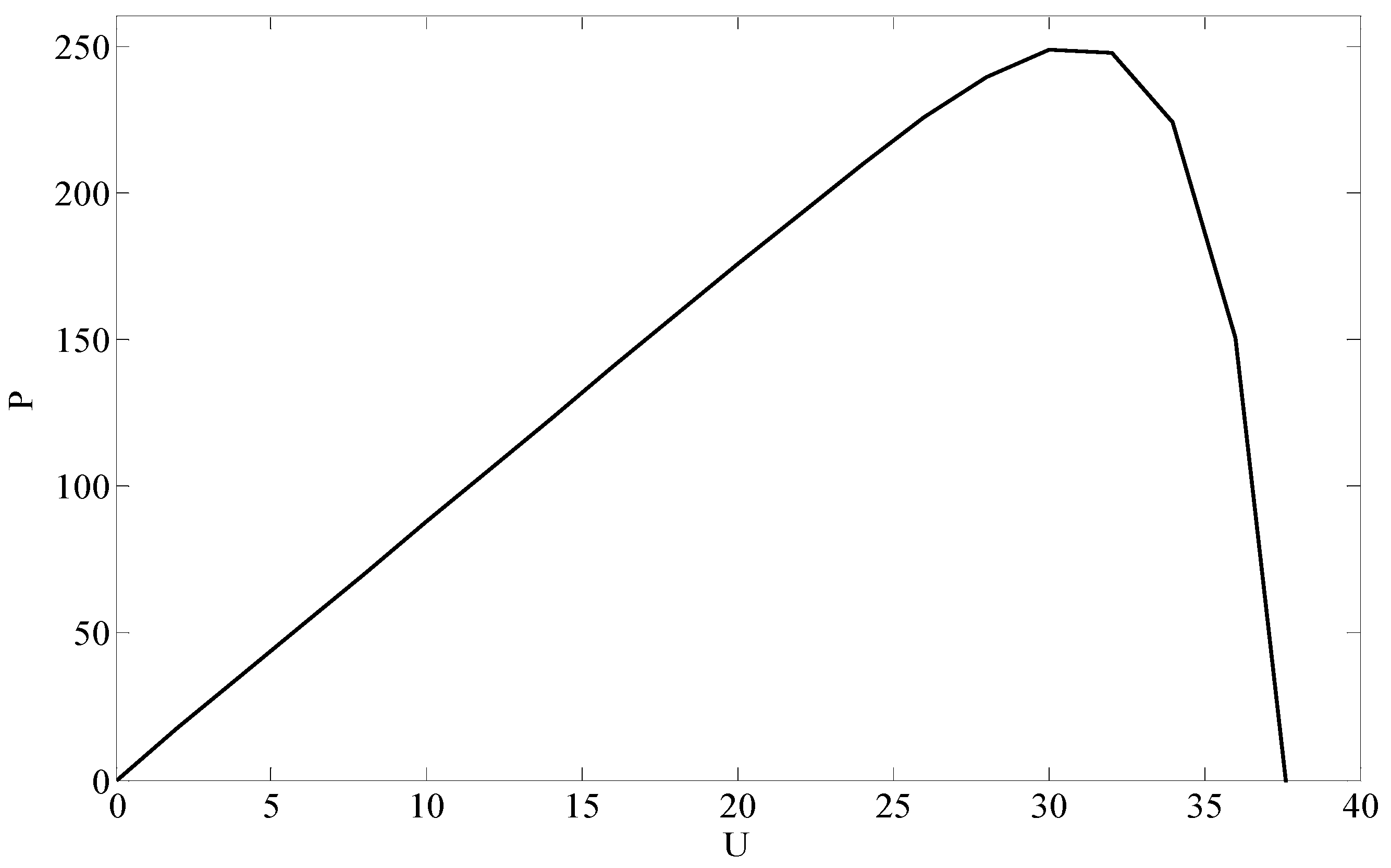
Since environmental factors can easily affect the PV arrays, its working point is going to vary. Figure 4 plots the P-U characteristics of PV cells. The maximum power point is the peak of the P-U characteristic curve of PV cell, satisfying the following condition:

$$\frac{dP}{d{U}_{pv}}=\frac{d(U_{pv}{I}_{pv})}{U_{pv}}=I_{pv}+U_{pv}\frac{d{I}_{pv}}{d{U}_{pv}}=0$$

(8)

which can be rewritten as:

$$\frac{d{I}_{pv}}{d{U}_{pv}}=-\frac{I_{pv}}{U_{pv}}$$

(9)

From Section 2, unit A, it is known that the boost chopper satisfies: $u_{pv}=(1-D_b)u_{dc}$, where the duty cycle of the power switch S is $D_b$, the output voltage is $u_{pv}$, and the output of the boost part is $u_{dc}$. When $u_{dc}$ is kept constant, $u_{pv}$ and $D_b$ will change inversely. The work point of PV arrays can be changed by adjusting $D_b$.

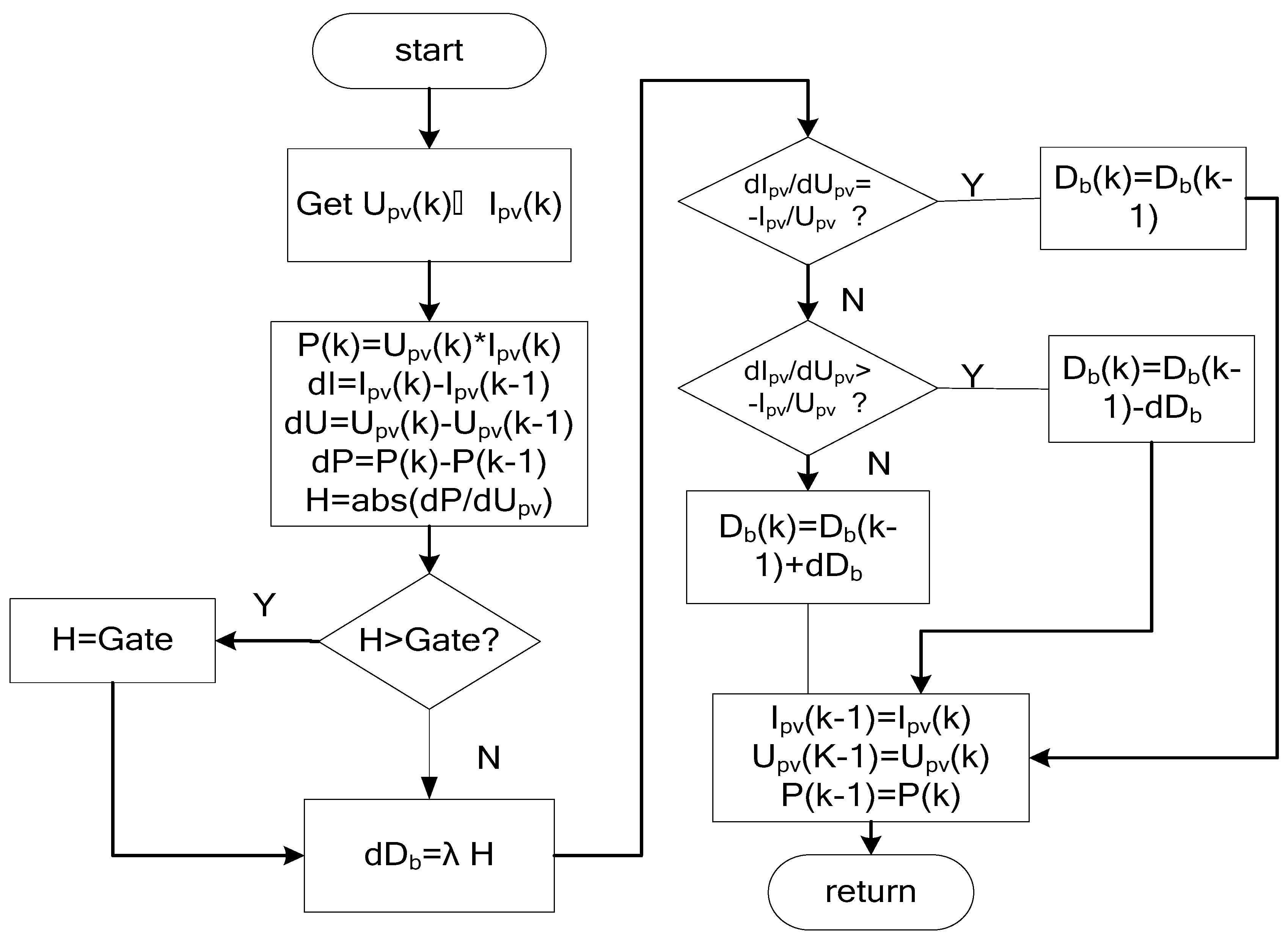
Using the adaptive step size as $\lambda \left|\frac{dP}{d{U}_{pv}}\right|$, where $\lambda$ is a positive constant, then the iteration algorithm of INC with this step size can be expressed as:

$$D_b(k)=D_b(k-1)\pm \lambda \left|\frac{dP}{d{U}_{pv}}\right|$$

(10)

The position of the current point determines the sign in Equation (9). Moreover, in order to avoid too large a step, a threshold is set for the step size. Figure 5 describes the algorithm INC with adaptive size in detail.

4. Adaptive Fuzzy Sliding Mode Control

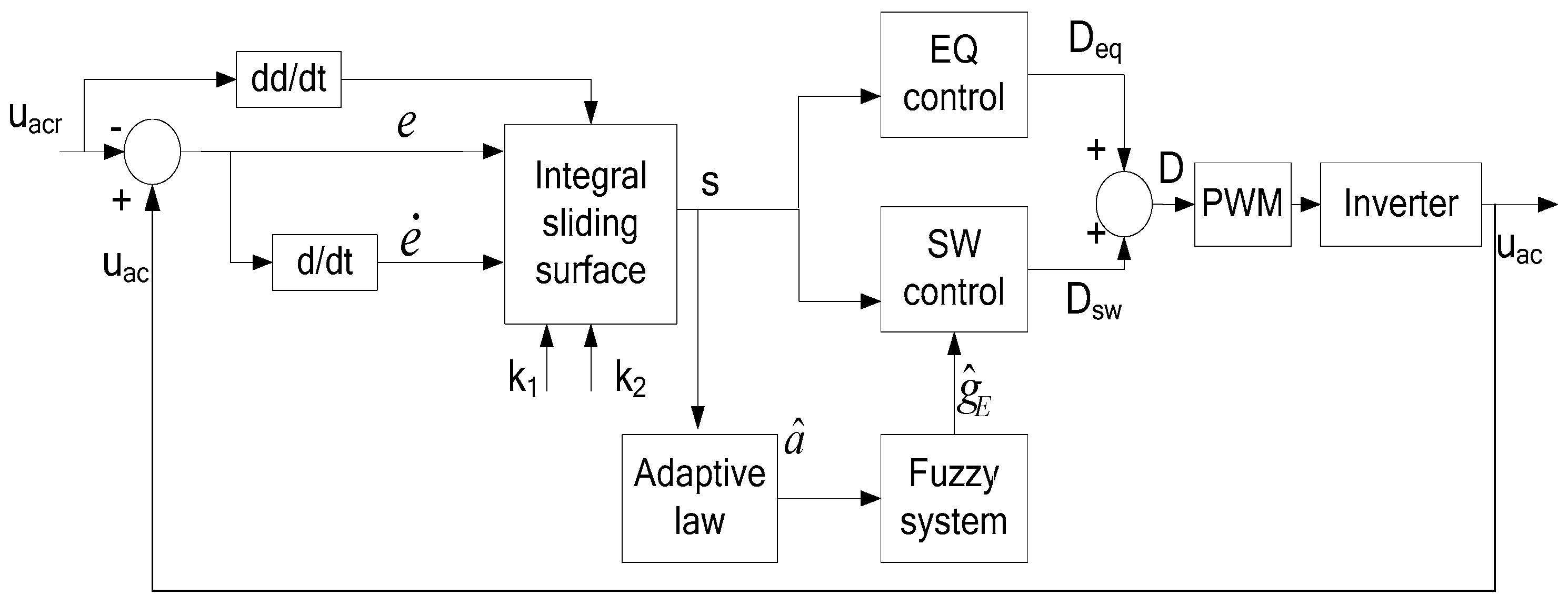
A grid-connected PV inverter is used to guarantee that the output voltage of the inverter can follow the grid reference voltage. The block diagram of the AFSMC algorithm is shown in Figure 6. First, an integral sliding surface is selected, then the equivalent (EQ) controller is calculated by setting $\dot{s}=0$ without the nonlinearities. The total control is composed of the EQ controller and a switching (SW) controller that is employed to compensate the unknown nonlinearities. Finally, a fuzzy controller is used to estimate the upper bound of the nonlinearities in the switching (SW) controller. Then, the controller output is transferred to the Pulse Width Modulation (PWM) to control the inverter. The output of the inverter U_ac is used as a feedback signal to the reference input U_acr to constitute a tracking error signal.

4.1. Sliding Mode Control

An integral sliding surface is designed as in Equation (11):

$$s(t)={\dot{u}}_{ac}(t)-{\displaystyle \underset{0}{\overset{t}{\int }}[{\ddot{u}}_{acr}(t)-k_1\dot{e}(t)-k_{2}e(t)]dt}$$

(11)

where $u_{acr}$ is the grid reference voltage, $e=u_{ac}-u_{acr}$ is the tracking error between $u_{ac}$ and $u_{acr}$, and $k_1$ and $k_2$ are positive constants.

The derivative of the integral sliding surface becomes:

$$\dot{s}=-\frac{1}{R_L{C}_{ac}}{\dot{u}}_{ac}-\frac{1}{L_{ac}{C}_{ac}}{u}_{ac}+\frac{2D-1}{L_{ac}{C}_{ac}}{u}_{dc}+g-{\ddot{u}}_{acr}+k_1\dot{e}+k_{2}e$$

(12)

Ignoring the system nonlinearities and setting $\dot{s}=0$ and $g$ yields the equivalent controller $D_{eq}$ as:

$$D_{eq}=0.5[1+\frac{L_{ac}{C}_{ac}}{u_{dc}}(\frac{1}{R_L{C}_{ac}}{\ddot{u}}_{ac}+\frac{1}{L_{ac}{C}_{ac}}{u}_{ac}+{\ddot{u}}_{acr}-k_1\dot{e}-k_{2}e)]$$

(13)

Then, considering the system nonlinearity, a comprehensive controller is proposed as:

$$D=D_{eq}+D_{sw}$$

(14)

$$D_{sw}=-0.5*\frac{L_{ac}{C}_{ac}}{u_{dc}}{g}_E\mathrm{sgn}(s)$$

(15)

where $\left|g\right|<g_E$, $g_E$ is the upper bound of the system nonlinearities, and sgn(s) is the sign of s. The sliding controller is designed to compensate for the unknown nonlinearities to satisfy the sliding condition.

4.2. Adaptive Fuzzy Sliding Mode Control

Since it is difficult to measure the upper bound of nonlinearities in practical applications, a fuzzy system is proposed to adaptively estimate the optimal upper bound of the nonlinearities.

The tracking error $e$ is selected as the input of the fuzzy controller, and the upper bound of the uncertainties is its output.

According to the universal approximation theory, there exists an optimal parameter satisfying $g^{*}{}_E=g_E+\epsilon =a^{*}{}^T\xi$, where $a$ is an adjustable parameter, $a^{*}$ is an optimal parameter, $\xi$ is a fuzzy basis function vector, and ${\xi }_i=\frac{w_i}{{\displaystyle \sum w_i}}$, i = 1,2,3 ....... m, $\epsilon$ is the approximation error bounded by $\left|\epsilon \right|<E$, where E is a positive constant.

A fuzzy system ${\widehat{g}}_E$ is employed to approximate the upper bound of system nonlinearities as:

$${\widehat{g}}_E={\widehat{a}}^T\xi$$

(16)

where $\widehat{a}$ is the estimation of $a^{*}$.

Replacing $g_E$ in Equation (15) by ${\widehat{g}}_E$ and combining Equations (13) and (14) yields the new controller as Equation (17):

$$D=0.5[1+\frac{L_{ac}{C}_{ac}}{u_{dc}}(\frac{1}{R_L{C}_{ac}}{\ddot{u}}_{ac}+\frac{1}{L_{ac}{C}_{ac}}{u}_{ac}+{\ddot{u}}_{acr}-k_1\dot{e}-k_{2}e-{\widehat{g}}_E\mathrm{sgn}(s))]$$

(17)

Substituting Equation (17) into Equation (12) obtains:

$$\dot{s}=g-{\widehat{g}}_E\mathrm{sgn}(s)$$

(18)

Define $\tilde{a}=\widehat{a}-a^{*}$ as the estimation error.

Selecting a Lyapunov function as:

$$V=\frac{1}{2}{s}^2+\frac{1}{2\eta }{\tilde{a}}^T\tilde{a}$$

(19)

where $\eta$ is a positive constant.

The derivative of V becomes:

$$\begin{array}{ll}\dot{V}& =s\dot{s}+\frac{1}{\eta }{\tilde{a}}^T\dot{\tilde{a}}\\ & =s(g-{\widehat{g}}_E\mathrm{sgn}(s))+\frac{1}{\eta }{\tilde{a}}^T\dot{\tilde{a}}\\ & =s(g-{\widehat{a}}^T\xi \mathrm{sgn}(s))+\frac{1}{\eta }{(\widehat{a}-a^{*})}^T\dot{\tilde{a}}\\ & =sg-{\widehat{a}}^T\xi \left|s\right|+\frac{1}{\eta }{(\widehat{a}-a^{*})}^T\dot{\tilde{a}}\end{array}$$

(20)

An adaptive law can be obtained as:

$$\dot{\widehat{a}}=\dot{\tilde{a}}=\eta \left|s\right|\xi$$

(21)

Substituting Equation (21) into Equation (20) yields:

$$\begin{array}{ll}\dot{V}& =sg-\left|s\right|a^{*T}\xi \\ & \le \left|s\right|g-\left|s\right|a^{*T}\xi \\ & =-(g_E-g+\epsilon )\left|s\right|\\ & \le 0\end{array}$$

(22)

$\dot{V}$ is negative semi-definite, which implies that the closed-loop system is asymptotically stable, where $V\to 0$ as $t\to \infty$, and therefore $e\to 0$ as $t\to \infty$, meaning the output of inverter can track the grid reference voltage.

5. Adaptive Fuzzy Neural Network Terminal Sliding Mode Control

Terminal sliding mode with a nonlinear sliding surface has a good property to converge to an equilibrium state in a finite time.

5.1. Sliding Surface Design

Define the tracking error as:

$$e=u_{ac}-u_{acr}$$

(23)

where $u_{ac}$ is the output voltage of the DC-AC inverter, and $u_{acr}$ is the grid reference voltage.

A global fast terminal sliding function is designed as:

$$s=\dot{e}+\alpha e+\beta e^{\frac{q}{p}}$$

(24)

where $\alpha ,\beta$ are both are positive constants, and $p,q(p>q)$ are positive integers. Note that $p$ and $q$ must be odd integers so that for any real number $e$, $\beta e^{\frac{q}{p}}$ is always a real number.

When $s=0$, the system dynamics is expressed by the following differential equation:

$$s=\dot{e}+\alpha e+\beta e^{\frac{q}{p}}=0$$

(25)

The convergence rate is mainly determined by the nonlinear term $\beta e^{\frac{q}{p}}$. By properly choosing $\alpha ,\beta ,p,q$, for any initial state $e(0)\ne 0$, the dynamics of Equation (25) will reach $e=0$ in a finite time. In addition, by solving Equation (25), the exact time to converge to an equilibrium state from any initial state $t_s$ is derived as:

$$t_s=\frac{p}{\alpha (p-q)}\ln \frac{\alpha e{(0)}^{(p-q)/p}+\beta }{\beta }$$

(26)

5.2. Global Fast Terminal Sliding Mode Control

A global fast terminal sliding controller is designed for the inverter in this part.

Select a Lyapunov function candidate as given in Equation (27):

$$V_1=\frac{1}{2}{s}^2$$

(27)

The derivative of $V_1$ is

$$\begin{array}{ll}{\dot{V}}_1& =s(\ddot{e}+\alpha \dot{e}+\beta \frac{q}{p}{e}^{\frac{q}{p}-1}\dot{e})\\ & =s(\ddot{e}+(\alpha +\beta \frac{q}{p}{e}^{\frac{q}{p}-1})\dot{e})\\ & =s({\ddot{u}}_{ac}-{\ddot{u}}_{acr}+(\alpha +\beta \frac{q}{p}{e}^{\frac{q}{p}-1})\dot{e})\\ & =s(-\frac{1}{R_L{C}_{ac}}{\dot{u}}_{ac}-\frac{1}{L_{ac}{C}_{ac}}{u}_{ac}+\frac{2D-1}{L_{ac}{C}_{ac}}{u}_{dc}\\ & +g-{\ddot{u}}_{acr}+(\alpha +\beta \frac{q}{p}{e}^{\frac{q}{p}-1})\dot{e})\end{array}$$

(28)

A control law is designed as:

$$D=0.5[1+\frac{L_{ac}{C}_{ac}}{u_{dc}}(\frac{1}{R_L{C}_{ac}}{\dot{u}}_{ac}+\frac{1}{L_{ac}{C}_{ac}}{u}_{ac}+{\ddot{u}}_{acr}-(\alpha +\beta \frac{q}{p}{e}^{\frac{q}{p}-1})\dot{e}-g_E\mathrm{sgn}(s)-k\cdot s)]$$

(29)

where $g_E>|g{|}_{\max }$, $g_E$ is the upper bound of the system uncertainties, and $k\cdot s$ is a linear compensation term, where $k$ is a positive constant.

Applying Equation (29) to Equation (28) gives:

$$\begin{array}{l}\dot{V}=s(g-g_E\mathrm{sgn}(s)-ks)\\ =sg-\left|s\right|g_E-k{s}^2\\ \le \left|s\right|{\left|g\right|}_{\max }-\left|s\right|g_E-k{s}^2\\ =-(g_E-{\left|g\right|}_{\max })\left|s\right|-k{s}^2\le 0\end{array}$$

(30)

${\dot{V}}_1$ is negative semi-definite, guaranteeing the stability of the system.

5.3. Fuzzy Neural Network Global Fast Terminal Sliding Mode Control

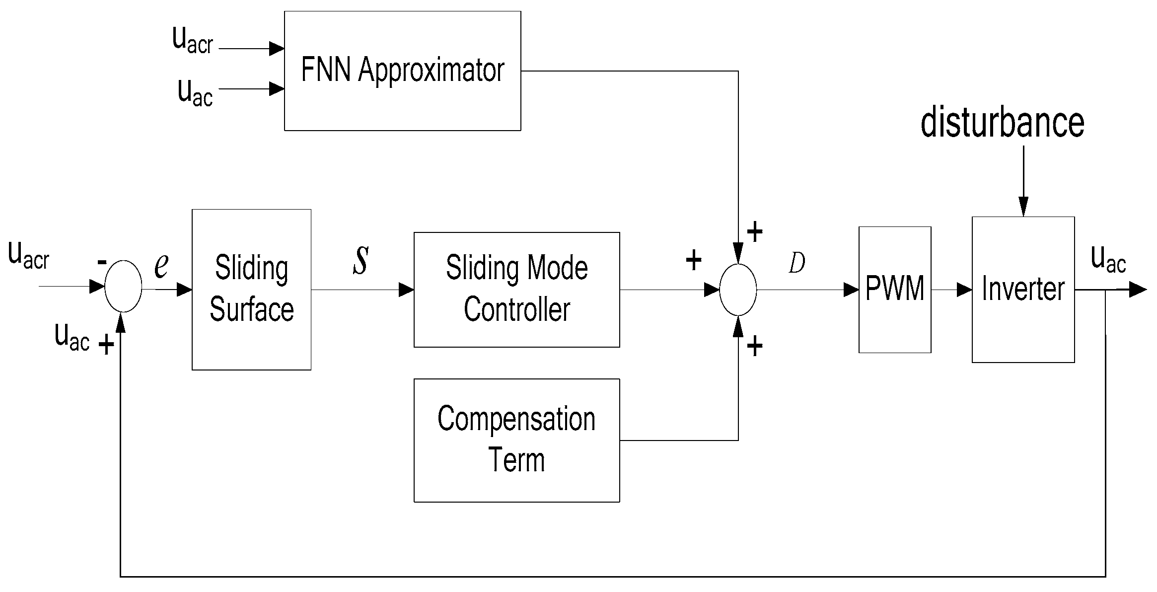
The block diagram of the proposed FNNGFTSMC structure is described in Figure 7. The output of FNN $\widehat{g}$ is designed to approximate the system uncertainties $g$ as:

$$\widehat{g}=w^T\xi (x)$$

(31)

where $w$ gives the connection weights of FNN, and $x=[u_{ac} u_{acr}]$ is the input vector.

The global fast terminal sliding controller with FNN to estimate the system uncertainties $g$ is proposed as in Equation (32):

$$D=0.5[1+\frac{L_{ac}{C}_{ac}}{u_{dc}}(\frac{1}{R_L{C}_{ac}}{\dot{u}}_{ac}+\frac{1}{L_{ac}{C}_{ac}}{u}_{ac}+{\ddot{u}}_{acr}-(\alpha +\beta \frac{q}{p}{e}^{\frac{q}{p}-1})\dot{e}-\widehat{g}-k\cdot s-{\epsilon }_m\mathrm{sgn}(s))]$$

(32)

where $\widehat{g}$ is the estimation value of $g$, $k$ is a positive constant, and ${\epsilon }_m>|\epsilon {|}_{\max }$, where $|\epsilon {|}_{\max }$ is a positive constant

The derivative of the sliding function, Equation (24), is:

$$\begin{array}{ll}\dot{s}& =\ddot{e}+\alpha \dot{e}+\beta \frac{q}{p}{e}^{\frac{q}{p}-1}\dot{e}\\ & =\ddot{e}+(\alpha +\beta \frac{q}{p}{e}^{\frac{q}{p}-1})\dot{e}\\ & ={\ddot{u}}_{ac}-{\ddot{u}}_{acr}+(\alpha +\beta \frac{q}{p}{e}^{\frac{q}{p}-1})\dot{e}\\ & =-\frac{1}{R_L{C}_{ac}}{\dot{u}}_{ac}-\frac{1}{L_{ac}{C}_{ac}}{u}_{ac}+\frac{2D-1}{L_{ac}{C}_{ac}}{u}_{dc}\\ & +g-{\ddot{u}}_{acr}+(\alpha +\beta \frac{q}{p}{e}^{\frac{q}{p}-1})\dot{e}\end{array}$$

(33)

Applying Equation (32) to Equation (33) yields:

$$\dot{s}=g-\widehat{g}-k\cdot s-{\epsilon }_m\mathrm{sgn}(s)$$

(34)

Selecting a Lyapunov function candidate as:

$$V=\frac{1}{2}{s}^2+\frac{1}{2r}{\tilde{w}}^T\tilde{w}$$

(35)

where $\tilde{w}=\widehat{w}-w^{\ast }$ is the estimation error, and $r$ is a positive constant.

The derivative of Equation (35) becomes:

$$\begin{array}{l}\dot{V}=s\dot{s}+\frac{1}{r}{\tilde{w}}^T\dot{\tilde{w}}\\ =s(g-\widehat{g}-k\cdot s-{\epsilon }_m\mathrm{sgn}(s))+\frac{1}{r}{\tilde{w}}^T\dot{\tilde{w}}\\ =s(g^{\ast }+\epsilon -\widehat{g}-k\cdot s)-{\epsilon }_m\left|s\right|+\frac{1}{r}{\tilde{w}}^T\dot{\tilde{w}}\\ =s(g^{\ast }-\widehat{g})+s\epsilon -k{s}^2-{\epsilon }_m\left|s\right|+\frac{1}{r}{\tilde{w}}^T\dot{\tilde{w}}\\ =-s{\tilde{w}}^T\xi +s\epsilon -k{s}^2-{\epsilon }_m\left|s\right|+\frac{1}{r}{\tilde{w}}^T\dot{\tilde{w}}\end{array}$$

(36)

An adaptive law is designed as:

$$\dot{\tilde{w}}=\dot{\widehat{w}}=rs\xi$$

(37)

Substituting Equation (37) into Equation (36) results in:

$$\begin{array}{l}\dot{V}=s\epsilon -{\epsilon }_m\left|s\right|-k{s}^2\\ \le \left|s\right|\epsilon -{\epsilon }_m\left|s\right|-k{s}^2\\ =-({\epsilon }_m-\epsilon )\left|s\right|-k{s}^2\le 0\end{array}$$

(38)

$\dot{V}$ is negative semi-definite, which ensures that $V,s,\dot{s}$ are all bounded, and $V(t)<V(0)<\infty$. Furthermore, $\dot{V}\le -k{s}^2$ implies that s is square-integrable as ${\displaystyle {\int }_0^t{s}^2}dt\le \frac{1}{k}(V(0)-V(t))$. Since $\dot{s}$ is bounded, according to the Barbalat lemma, $s\to 0$ as $t\to \infty$.

6. Simulation Results and Discussion

A grid-connected PV inverter is built in MATLAB/Simulink with SimPower Systems Toolbox (Figure 8) to verify the feasibility of the proposed strategies.

The PV module is composed of two 250 W photovoltaic components connected in series with the parameters as:

$I_{sc}=8.81 \mathrm{A}$, $I_m=8.36 \mathrm{A}$, $V_m=29.9 \mathrm{V}$, $V_{oc}=37.3 \mathrm{V}$. Boost chopper component parameters are set as $C_{pv}={10}^{-3} \mathrm{F}$, $L=3\times {10}^{-4} \mathrm{H}$, and $C_{dc}={10}^{-4} \mathrm{F}$. Parameters of the DC-AC inverter are chosen as $L_{ac}=0.048 \mathrm{H},C_{ac}=2\times {10}^{-5} \mathrm{PF}$, $R_L=400 \mathsf{\Omega }$. In the MPPT strategy, Φ = 60, $\lambda ={10}^{-6}$.

The FNNGFTSMC parameters are chosen as $\alpha =8000$, $\beta =10$, $p=5$, and $q=1$. The grid reference voltage is sinusoidal with a frequency 50 Hz and amplitude 311 V.

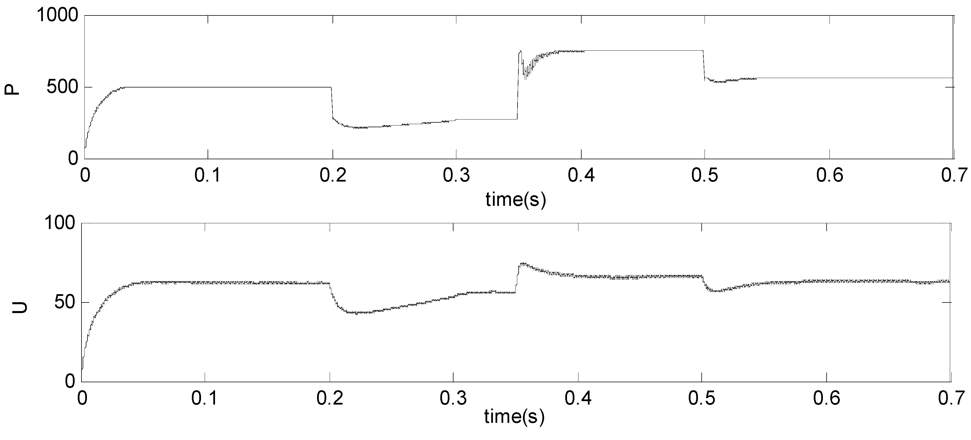
6.1. MPPT Performance

The environment of the PV inverter often changes. The initial insolation level is set to be 880 w/m² (88%), and at time 0.25 s, it is changed from 880 w/m² to 1000 w/m² (100%), and again at time 0.4 s, it is changed to 740 w/m² (74%).

Figure 9 shows that the power of PV modules was greatly determined by the insolation level, proving the effectiveness of the proposed MPPT strategy.

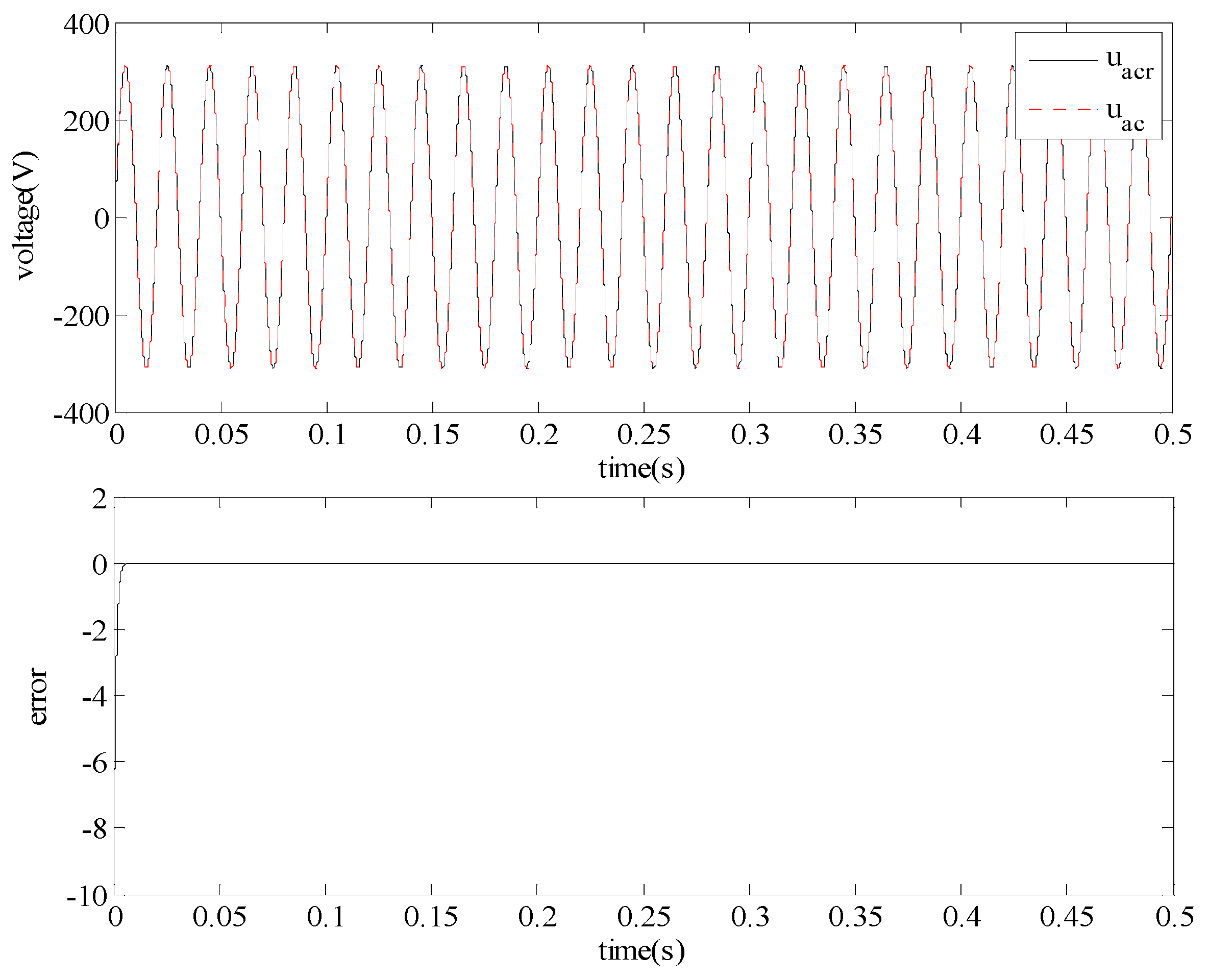
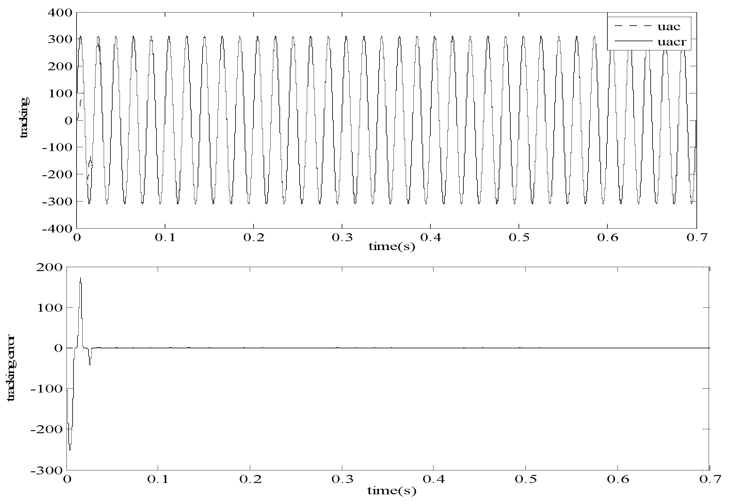
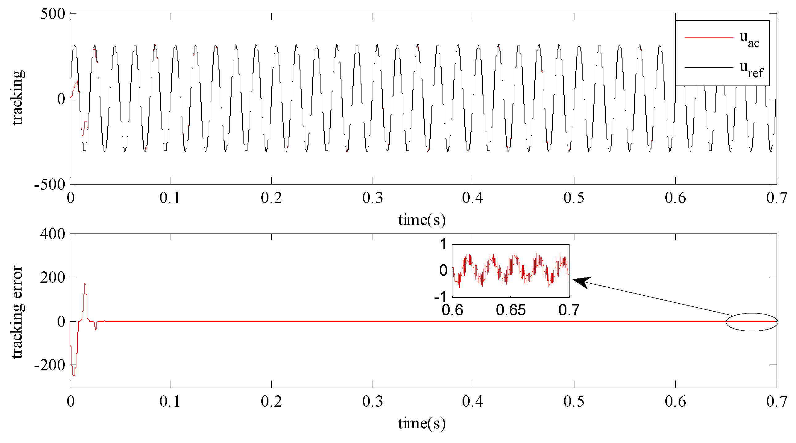
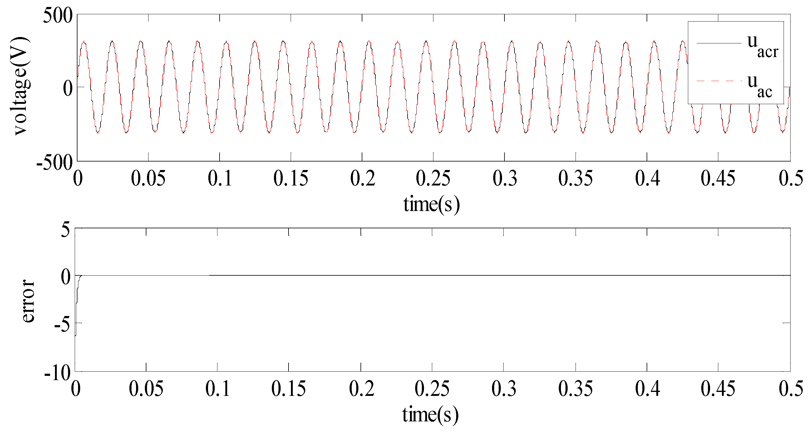
Figure 10 and Figure 11 show the performance of the proposed FNNGFTSMC scheme and AFSMC scheme, respectively, where the solid line ($u_{acr}$) is the reference voltage, and the dotted line $u_{ac}$ is the output voltage. The proposed FNNGFTSMC and AFSMC strategies can achieve a reliable grid-connection, the voltage tracking error converges to zero, and the proposed strategy has strong robustness to environment variations.

6.2. Performance of Inverter

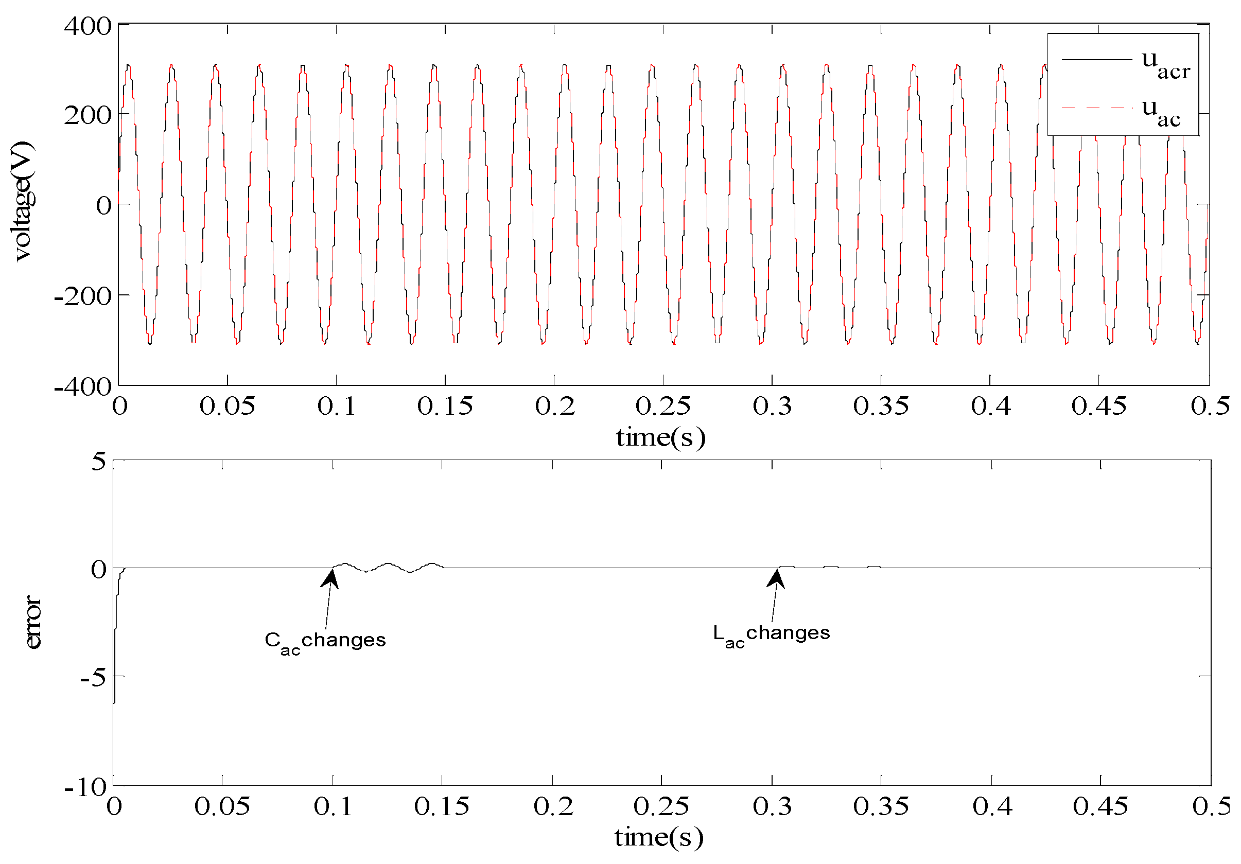
6.2.1. Parameter Variations

When t = 0.1–0.15 s, a random disturbance $2\times {10}^{-6} rand(1)$ PF is added to the capacitance parameter $C_{ac}$, and while t = 0.3–0.35 s, the inductance parameter varies by adding a random disturbance with amplitude ${10}^{-3}$, shown in Figure 12.

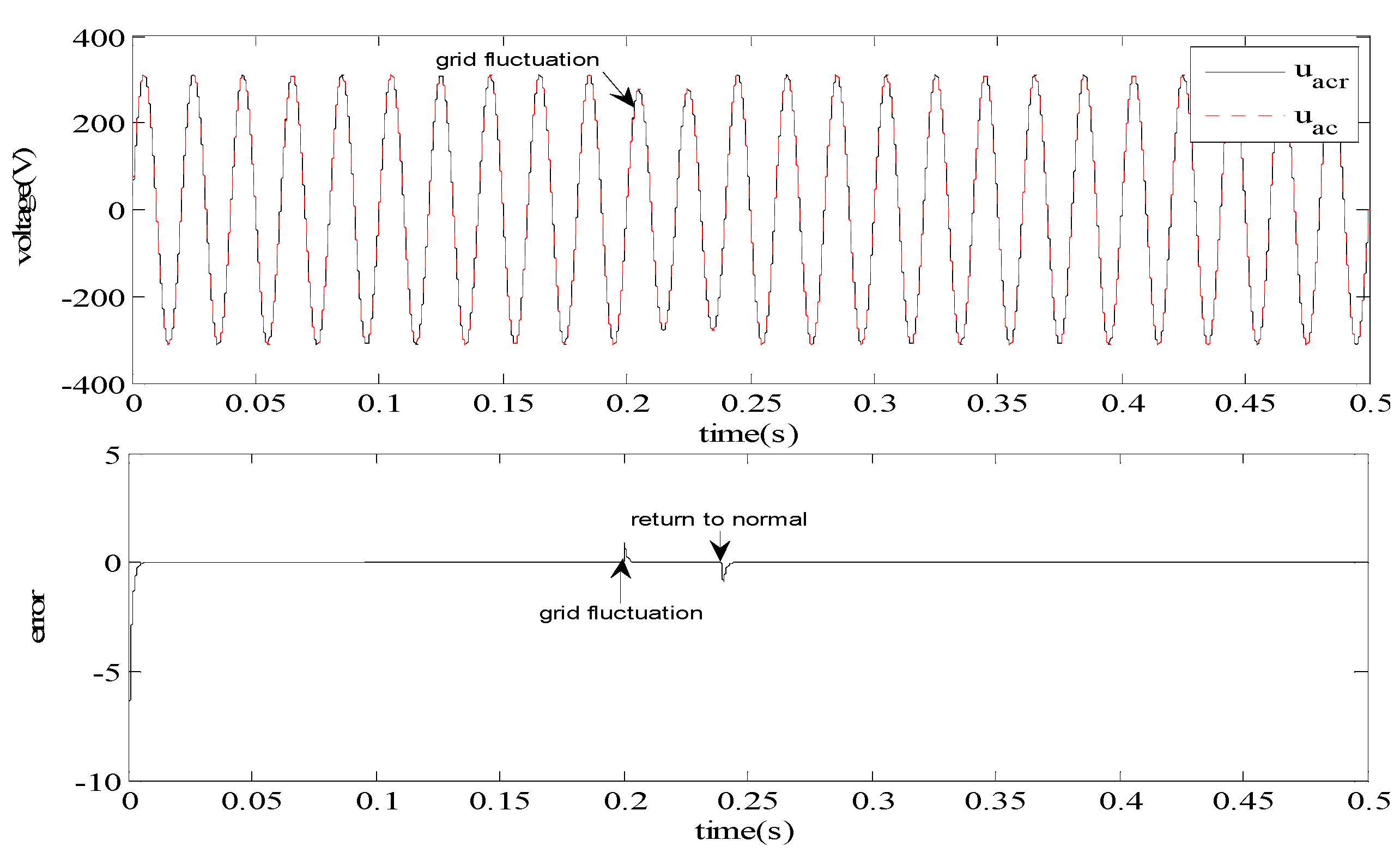
6.2.2. Voltage Fluctuation in the Grid Side

Voltage fluctuation in the grid side is tested at time 0.2 s, the grid voltage varies from 311 V to 280 V, and then returns to a normal level (311 V) at time 0.24 s. Figure 13 shows the adaptabilities of the inverter under grid voltage fluctuation, showing the tracking error can decrease to zero quickly.

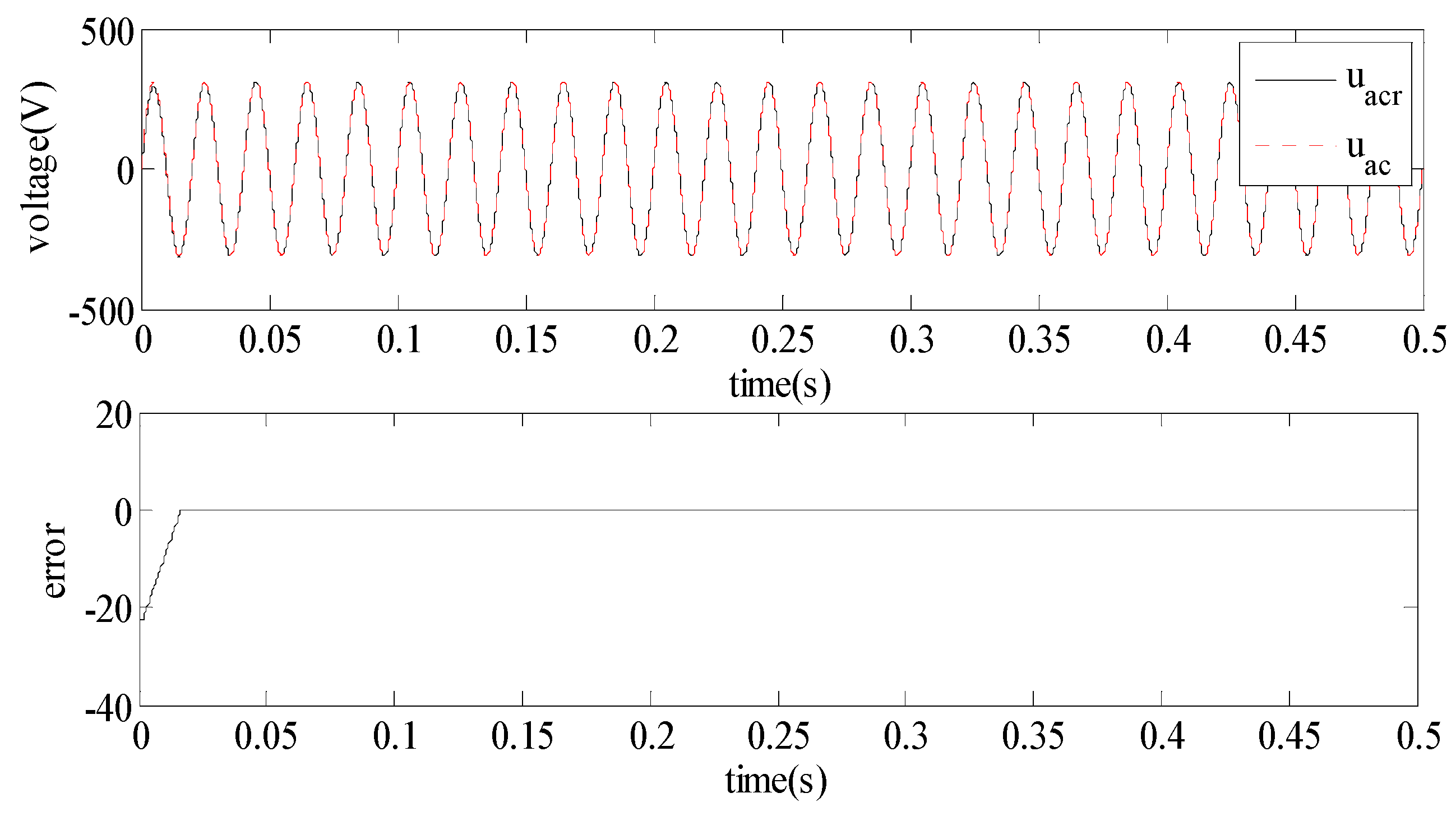
In order to study the advantages of the proposed controller, a comparison with sliding control is implemented under the same conditions. The sliding mode surface is designed as $s=\dot{e}+c\cdot e$, and the sliding term $\eta \mathrm{sgn}(s)$ is utilized to compensate for the influence of the system uncertainties. The parameters are $c=$ 4000 and $\eta =6\times {10}^6$. A random disturbance is added when t = 0.2–0.4 s. The comparisons of the steady performance for the inverter are studied in Figure 14, Figure 15 and Figure 16, showing the tracking error with SMC is much bigger than that with FNNGFTSMC and AFSMC.

7. Conclusions

This paper proposed an intelligent adaptive sliding mode scheme to make the inverter track the grid reference voltage. An AFSMC strategy is presented to control the DC-AC inverter, and the fuzzy system is employed to estimate the upper bound of the unknown system nonlinearities. The global fast terminal sliding mode control is utilized to make the tracking error in the inverter go to zero in a finite time. A simulation study is implemented to show the feasibility of the proposed strategies compared with the SMC method.

References

- Liu, F.; Duan, S.; Liu, F.; Liu, B.; Kang, Y. A variable step size INC MPPT method for PV systems. IEEE Trans. Ind. Electron. 2008, 55, 2622–2628. [Google Scholar]
- Teng, J.H.; Huang, W.H.; Hsu, T.A.; Wang, C.Y. Novel and Fast Maximum Power Point Tracking for Photovoltaic Generation. IEEE Trans. Ind. Electron. 2016, 63, 4955–4966. [Google Scholar] [CrossRef]
- Nabulsi, A.; Dhaouadi, R. Efficiency optimization of a DSP-based standalone PV system using fuzzy logic and dual-MPPT control. IEEE Trans. Ind. Inform. 2012, 8, 573–584. [Google Scholar] [CrossRef]
- Zaki, A.M.; Amer, S.I.; Mostafa, M. Maximum power point tracking for PV system using advanced neural networks technique. Int. J. Emerg. Technol. Adv. Eng. 2012, 2, 58–63. [Google Scholar]
- Manimekalai, P.; Kumar, R.; Raghavan, S. Enhancement of Fuzzy Controlled Photovoltaic-Diesel System with Battery Storage Using Interleaved Converter with Hybrid MPPT for Rural Home. J. Sol. Energy Eng. Trans. ASME 2015, 137, 061005. [Google Scholar] [CrossRef]
- Ishaque, K.; Salam, Z.; Amjad, M.; Mekhilef, S. An improved particle swarm optimization (PSO)-based MPPT for PV with reduced steady-state oscillation. IEEE Trans. Power Electron. 2012, 27, 3627–3638. [Google Scholar] [CrossRef]
- Chen, Y.K.; Yang, C.H.; Wu, Y.C. Robust fuzzy controlled photovoltaic power inverter with Taguchi method. IEEE Trans. Aerosp. Electron. Syst. 2002, 38, 940–954. [Google Scholar] [CrossRef]
- Fei, J.; Lu, C. Adaptive Fractional Order Sliding Mode Controller with Neural Estimator. J. Franklin Inst. 2018, 355, 2369–2391. [Google Scholar] [CrossRef]
- Cecati, C.; Ciancetta, F.; Siano, P. A multilevel inverter for photovoltaic systems with fuzzy logic control. IEEE Trans. Ind. Electron. 2010, 57, 4115–4125. [Google Scholar] [CrossRef]
- Fei, J.; Wang, T. Adaptive Fuzzy-Neural-Network Based on RBFNN Control for Active Power Filter. Int. J. Mach. Learn. Cybern. 2018, 1–12. [Google Scholar] [CrossRef]
- Chu, Y.; Fei, J. Dynamic Global PID Sliding Mode Control Using RBF Neural Compensator for Three-Phase Active Power Filter. Trans. Inst. Meas. Control 2018, 40, 3549–3559. [Google Scholar] [CrossRef]
- Kumar, N.; Saha, T.K.; Dey, J. Sliding-Mode Control of PWM Dual Inverter-Based Grid-Connected PV System: Modeling and Performance Analysis. IEEE J. Emerg. Sel. Top. Power Electron. 2016, 4, 435–444. [Google Scholar] [CrossRef]
- Dhar, S.; Dash, P.K. A new backstepping finite time sliding mode control of grid connected PV system using multivariable dynamic VSC model. Int. J. Electr. Power Energy Syst. 2016, 82, 314–330. [Google Scholar] [CrossRef]
- Arsalan, M.; Iftikhar, R.; Ahmad, I. MPPT for photovoltaic system using nonlinear backstepping controller with integral action. Sol. Energy 2018, 170, 192–200. [Google Scholar] [CrossRef]
- Fang, Y.; Fei, J.; Yang, Y. Adaptive Backstepping Design of a Microgyroscope. Micromachines 2018, 9, 338. [Google Scholar] [CrossRef]
- Fang, Y.; Fei, J.; Hu, T. Adaptive Backstepping Fuzzy Sliding Mode Vibration Control of Flexible Structure. J. Low Freq. Noise Vib. Act. Control 2018, 2018, 5276074. [Google Scholar] [CrossRef]
- Khazane, J.; Tissir, H. Achievement of MPPT by finite time convergence sliding mode control for photovoltaic pumping system. Sol. Energy 2018, 166, 13–20. [Google Scholar] [CrossRef]
- Naghmash, A.; Ahmad, I. Backstepping based non-linear control for maximum power point tracking in photovoltaic system. Sol. Energy 2018, 159, 134–141. [Google Scholar] [CrossRef]
- Dhas, B.G.S.; Deepa, S.N. Fuzzy logic based dynamic sliding mode control of boost inverter in photovoltaic application. J. Renew. Sustain. Energy 2015, 7, 043133. [Google Scholar] [CrossRef]
- Zhu, Y.; Fei, J. Disturbance Observer Based Fuzzy Sliding Mode Control of PV Grid Connected Inverter. IEEE Access 2018, 6, 21202–21211. [Google Scholar] [CrossRef]
- Fei, J.; Zhu, Y. Adaptive fuzzy sliding control of single-phase PV grid-connected inverter. PLoS ONE 2017, 12. [Google Scholar] [CrossRef] [PubMed]
- Zhu, Y.; Fei, J. Adaptive Global Fast Terminal Sliding Mode Control of Grid-connected Photovoltaic System Using Fuzzy Neural Network Approach. IEEE Access 2017, 5, 9476–9484. [Google Scholar] [CrossRef]
Figure 1.
Single-phase grid-connected PV inverter model.
Figure 2.
Boost DC-DC chopper.