Leakage Detection of a Spherical Water Storage Tank in a Chemical Industry Using Acoustic Emissions


School of IT Convergence, University of Ulsan, Ulsan 44610, Korea
*
Author to whom correspondence should be addressed.
Appl. Sci. 2019, 9(1), 196; https://0-doi-org.brum.beds.ac.uk/10.3390/app9010196
Submission received: 22 November 2018
/
Revised: 25 December 2018
/
Accepted: 3 January 2019
/
Published: 8 January 2019
(This article belongs to the Special Issue Fault Detection and Diagnosis in Mechatronics Systems)
Abstract
:Featured Application
The proposed work is based on acoustic emission measurements and a machine learning technique to develop an intelligent fault diagnosis system. This work can be used to find cracks in industrial components such as spherical tank and pressure vessel.
Abstract
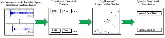
Spherical storage tanks are used in various industries to store substances like gasoline, oxygen, waste water, and liquefied petroleum gas (LPG). Cracks in the storage tanks are unaccepted defects, as storage tanks can leak or spill the contained substance through these cracks. Leakage from contained hazardous substances storage tanks can contaminate the environment and may lead to fatal accidents. Therefore, the ability to detect cracks from spherical storage tanks is necessary to avoid damage to the environment and to ensure public safety. In this paper, we present a crack detection case study of a spherical tank. The detection was performed using time-domain statistical features and a machine learning algorithm. The proposed method consists of (1) extraction of statistical features from the acoustic emissions (AE) acquired from the spherical tank, and (2) classification of the nonlinear data using a support vector machine (SVM). We evaluate the proposed algorithm with AE data obtained from the spherical tank, demonstrating that the algorithm effectively discriminates between normal and crack conditions. These results show that the proposed algorithm is effective for detecting cracks in spherical storage tanks.
1. Introduction
Spherical storage tanks are used in many industries, including the petrochemical, chemical, water management, and aerospace industries. They can store substances such as gasoline, oxygen, waste water, and liquefied petroleum gas (LPG) [1,2,3]. Along with the usefulness of storage tanks in industrial processes comes great responsibility. Installation of storage tanks in a facility can put environmental and public safety at risk when these tanks contain hazardous substances. Leaks through the cracks in storage tanks containing hazardous substances can pollute the air, land, and water [4]. This contamination of the environment can be fatal. Factors that can lead to leakage include cracks, corrosion, pipe failure, and poor maintenance. To avoid health risks, tank conditions must be monitored. Among the many ways to inspect the condition of a storage tank, the most popular and efficient are nondestructive testing methods, which have the primary advantages of not taking components out of operation during the integrity test, and not cutting them apart or altering them during the test [5]. The typical nondestructive testing methods include ultrasonic, radiographic, eddy current, electrical resistance measurement and acoustic emissions testing [6,7,8,9,10,11]. Among these methods, acoustic emission and electrical resistance measurements can detect early stage as well as already existing damages in an object. In the case of the electrical resistance method, when the failure stress is approached, the opening of the cracks cause variation of the electrical resistance. This variation indicates the initiation or presence of a crack and void in the structure. Similarly, when damage takes place in an object, it releases elastic waves which can be recorded as acoustic emission signals. These elastic waves (acoustic emission) also provide valuable information about the crack and plastic deformation in the object. Therefore, these two techniques can be used separately or in combination to address the issue of crack and leak detection in composites. In combination, acoustic emission testing can be used as primary means to detect cracks in an object, and then electrical resistance measurement of the object can be used to verify the results of acoustic emission testing. In this work, as the objective is to classify cracks of spherical tanks, acoustic emissions (AE) are just used as a means of nondestructive testing to record data regarding integrity testing of the spherical tank. AE testing has two main advantages: (1) No external energy is supplied in the AE recording; instead, the sound generated within the object is recorded. (2) AE testing can record dynamic changes in material, giving it the critical ability to discern growing and stagnant defects [5,12]. These advantages under real-time conditions make acoustic emission testing a favorable choice to acquire data regarding tank structural integrity. Moreover, AE testing provides wide-band signal recording, which makes the spectral analysis of the signals much easier. In this way, plastic deformation and microscopic leaks of a material can be investigated in real time.
Few quantitative approaches are described in the literature regarding the detection of spherical tank leakage as a classification problem. A study of leakage detection in a tank storing water for firefighting is presented in [13]. The authors examined AE waves acquired from a tank that had small holes at its bottom due to corrosion. They analyzed the fundamental characteristics of AE waves to identify the waves associated with the holes. A similar study [14] used wavelet neural networks to identify AE signals from different types of tanks. After employing a wavelet denoising algorithm, the signals were decomposed to a certain level, and the node energy distributions and extracted feature vectors from the corrosion signals were provided to the neural network to carry out the experiment.
In the current study, we considered the case of a spherical tank installed in chemical industry. The main objective of this work is to differentiate the AE signals obtained from the tank under normal and crack conditions: A binary classification problem. Quantitative assessment of signals has been carried out in many fields, such as speech recognition, natural language processing, and fault diagnosis [15,16,17,18,19,20,21]. We apply this concept to identify the structural integrity of a spherical tank. The current study has two main contributions: (1) Conversion of the AE signals into lower-dimensional feature space using time-domain statistical features, and (2) classification of nonlinear instances in the feature space by using a radial basis function (RBF) kernel-based support vector machine.
AE signals are collected from the storage tank under normal conditions (no crack) and under cracked conditions. Additionally, statistical features were extracted from the AE signals to quantify the signals from the two states and then input them to the support-vector-machine, which classifies the statistical features extracted from the AE signals. The results show that the proposed crack detection algorithm was able to correctly classify instances obtained from the spherical storage tank having crack.
2. Methodology
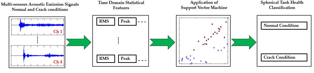
The methodology of this study is shown in Figure 1. It can be divided into two main steps. In the first step, statistical features were extracted from the AE signals acquired from the spherical tank under normal and cracked states. In the second step, these extracted statistical features were provided to SVM to identify whether each input instance belonged to the normal spherical tank or the cracked state.
2.1. Statistical Features
The acoustic emissions obtained from the spherical tank were time-domain measurements of the activity within the tank. These measurements consisted of voltage amplitude values taken at specific time intervals. Analyzing these measurements directly did not yield satisfactory results. Moreover, the sampling frequency of the measured signals was 1 MHz, and thus, each sample contained a huge number of data points. Therefore, quantification of the statistical features of the AE signals was needed to reduce the dimensions of the original data. Using time-domain statistical features, not only greatly reduces computational complexity, but also discriminated between the signals associated with the different structural integrity conditions in the feature space. The time-domain statistical features extracted from AE signals in this study consist of the peak (P), root mean square (RMS), kurtosis (K), crest factor (C), impulse factor (IF), shape factor (SF), skewness (S), square root mean (SRM), margin factor (MF), peak to peak (PP), kurtosis factor (KF), energy contained in the signals (E), and clearance factor (CF) values. The mathematical representation of these statistical features is given in Table 1.
2.2. Support Vector Machine (SVM)
A support vector machine is a popular machine-learning classifier that is used in mathematical and engineering problems, such as speech recognition, image processing, text classification, and natural language processing. The simplest form is a binary SVM classifier: One sorting instances into two classes.
Let us suppose there is a sample set consisting of , where . represents the length of the feature vectors and . Here, every is an -dimensional feature vector that belongs to one of the two classes, and , through , which defines the labels. Let us assume that the sample space is highly linearly separable. There are several approaches to linearly separate instances into two classes, for example, the use of a multilayer perceptron. Solutions to such problems are infinite sets depending on certain key factors, like a learning algorithm and its parameters, initial weights , and biases . Here, the focus of interest is to find the hyperplane that has the optimal separating margins between the two classes. The optimal margins provide a wide boundary between the classes, thereby reducing the misclassification rate.
If is highly linearly separable, then there exists a hyperplane and a positive that uniformly separate and ( is the dot product of vector and vector ). Therefore, any uniformly separating hyperplane can be represented by the following property:
A binary SVM classifier solves the following optimization problem:
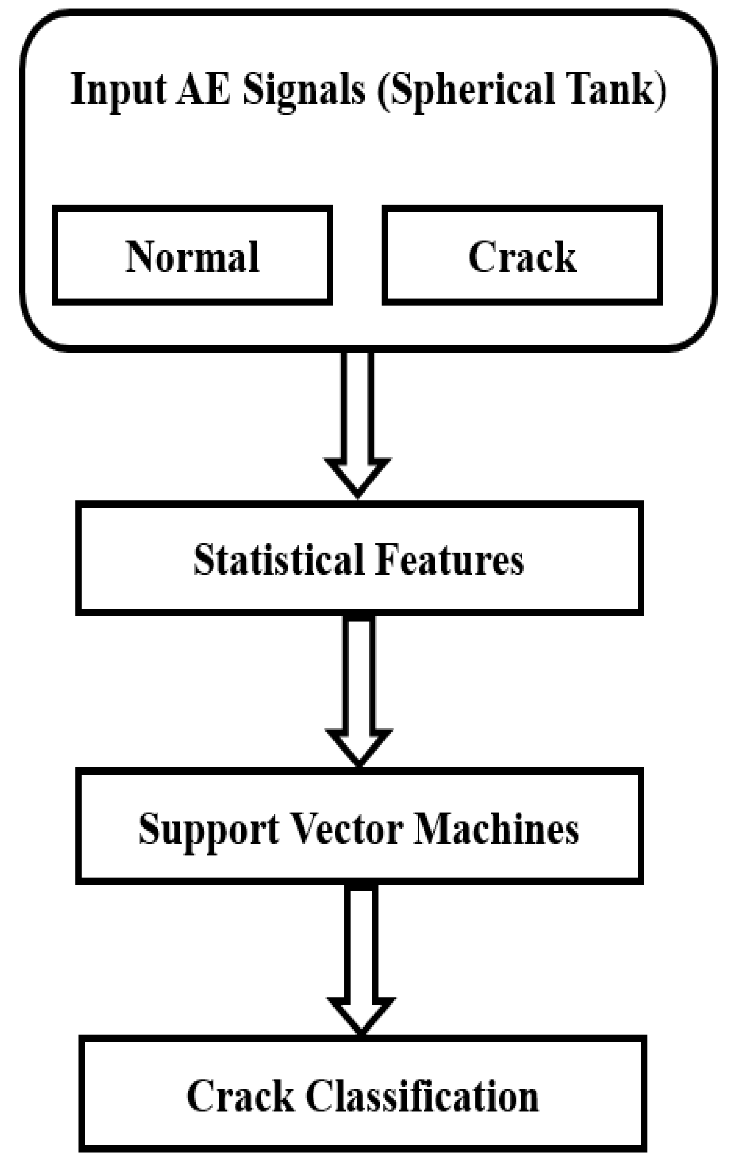
where are the Lagrange multipliers. Figure 2 presents the mechanism of how a hyperplane in the SVM separates two classes ( and ) that are linearly separable. Interestingly, the SVM can be changed from a linear to a nonlinear classifier by introducing a kernel function into the objective function. According to Cover’s theorem [22], if the data are not linearly separable into an input space , then it can be mapped to another feature space where the data are linearly separable. In this case, the main objective is to find a map function . The dot product in the new objective function is transformed into . If the condition is met by a kernel function , then the optimization problem will entirely depend on the function. Therefore, in the new feature space, we need to find linear margins. Thus, the optimization conditions can be generalized as follows:
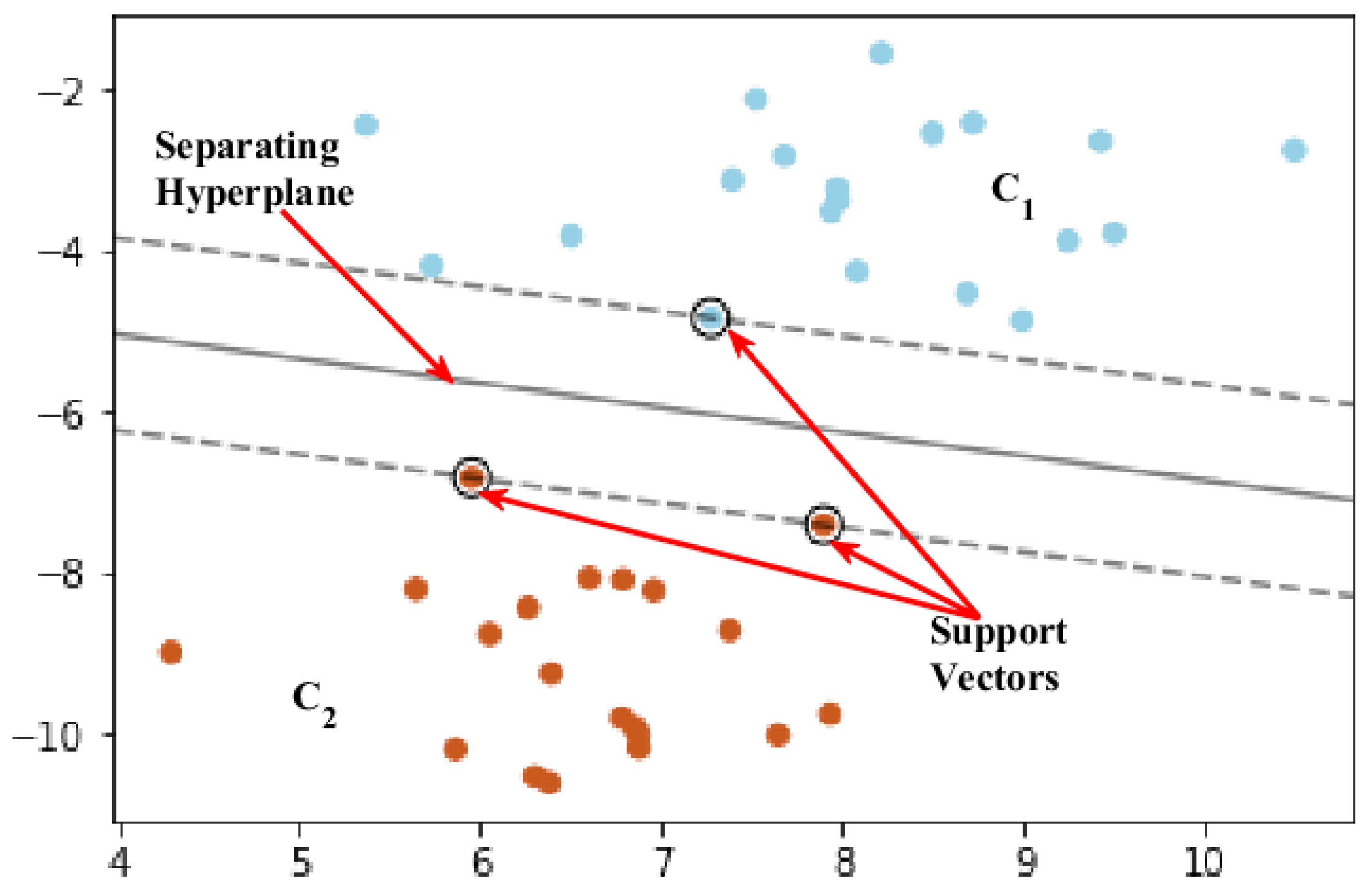
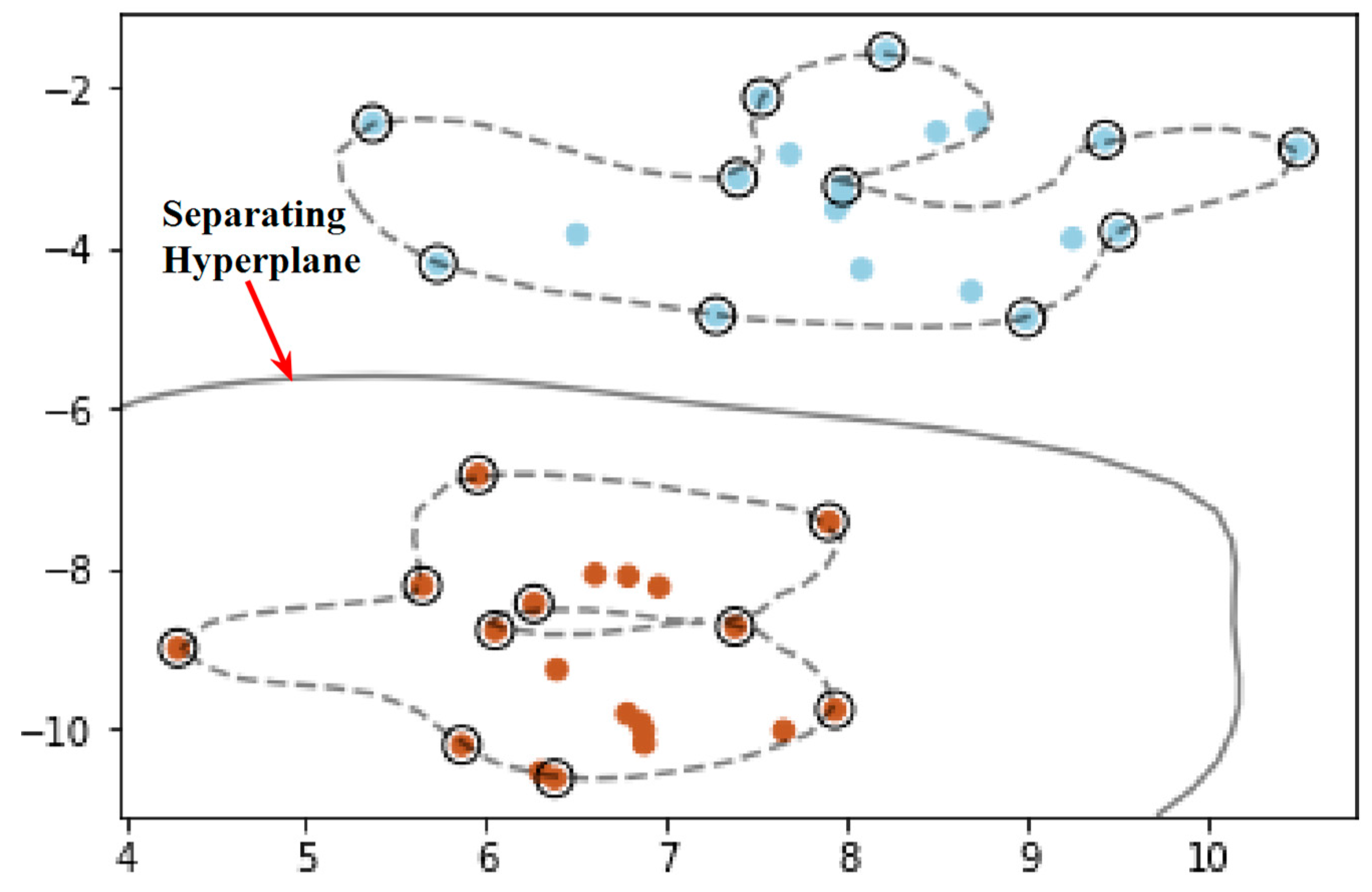
Here, the kernel function plays an important role. There are several kernel functions available for developing a nonlinear SVM. The most commonly used kernel functions are a dot product kernel, polynomial kernel, radial basis (Gaussian) kernel, and sigmoid kernel. In this work, we chose a Gaussian kernel function for training and testing the SVM. Figure 3 shows a hyperplane drawn between two nonlinear separable classes by using a Gaussian kernel function.
3. Dataset
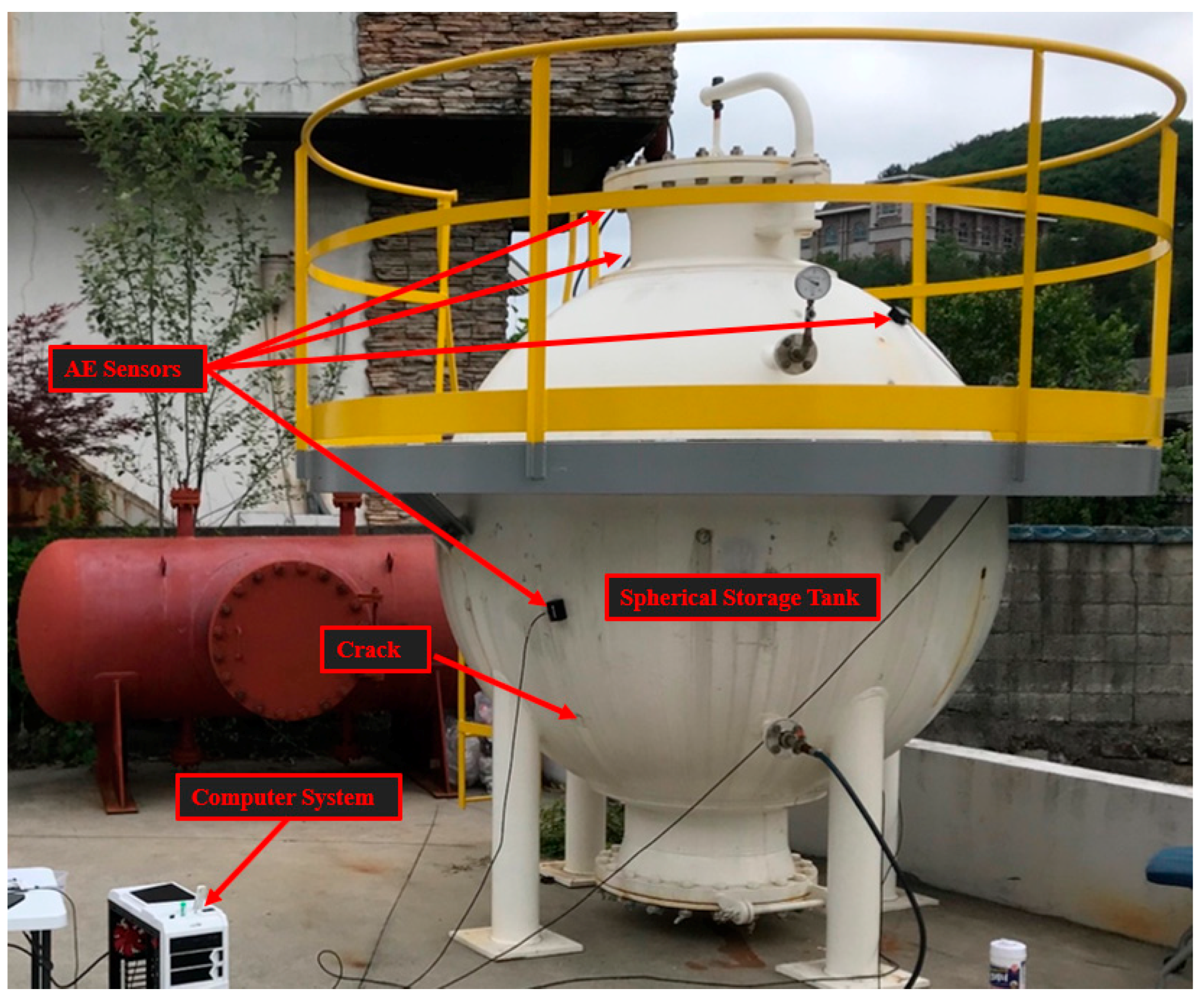
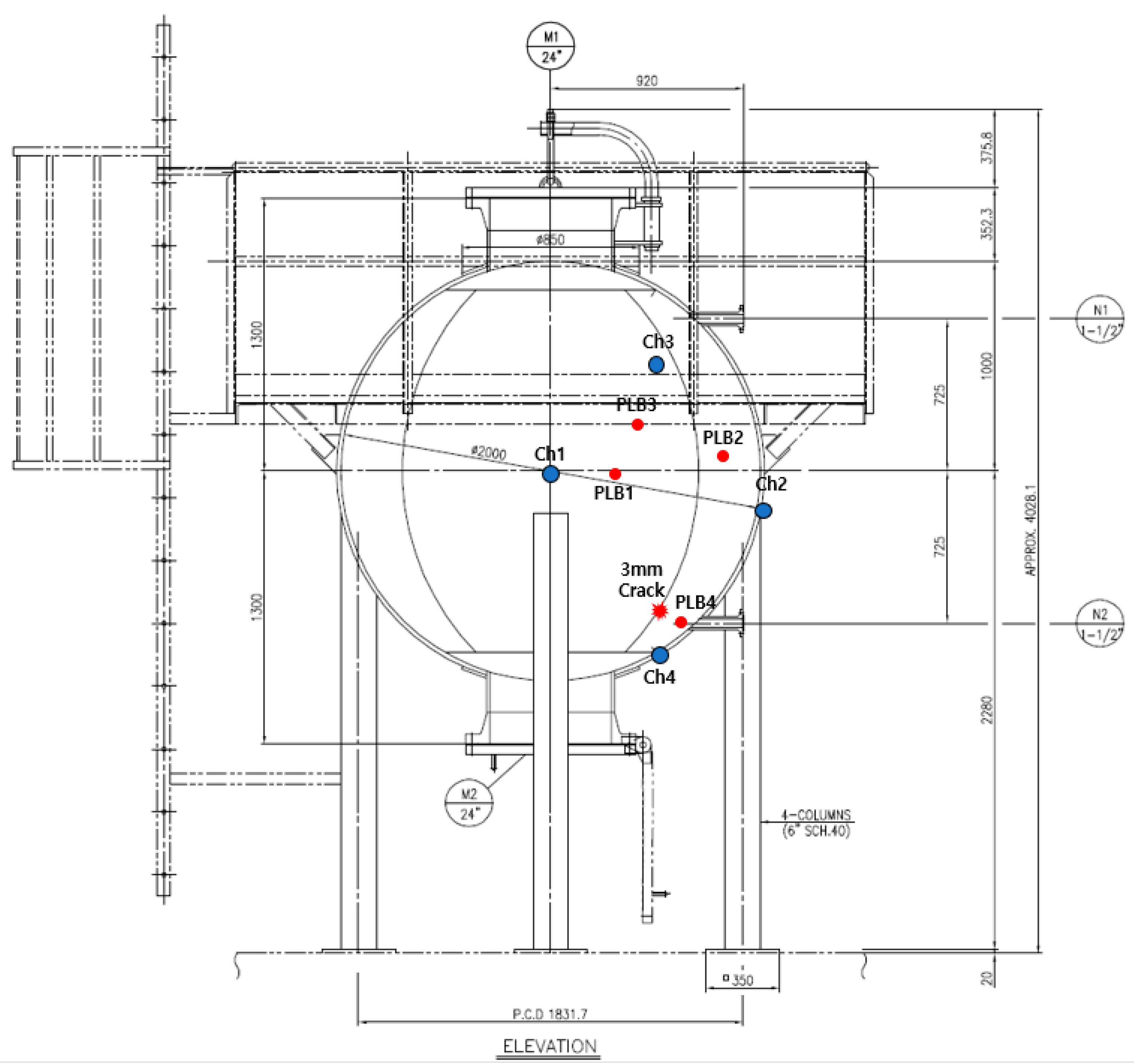
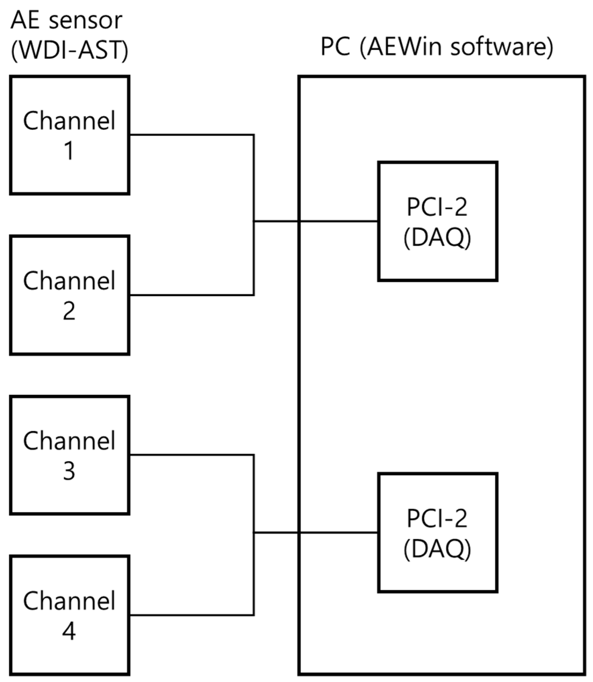
In our experiment, we considered a spherical tank made of carbon steel (A283-C) as a testbed. The testbed consisted of a spherical tank, AE sensors, a data acquisition device and a computer system, as presented in Figure 4. Moreover, for a detailed description, a schematic diagram of the test bed is also given in Figure 5. In the schematic diagram, the location of the four channels (sensors) and the pinhole crack can be easily observed. A 3-mm crack was deliberately introduced on the bottom of the tank. Four AE sensors were attached to the surface of the tank at different locations. A pencil lead test was performed to generate a guided wave through the tank surface. Acoustic emission signals were recorded using AE sensors keeping engineering norms in mind set by the American Society of Mechanical Engineers (ASME) and given in boiler and pressure vessel code (PVC) [23]. A peripheral component Interconnect bus (PCI-2) based data acquisition device connected with wideband differential AE sensors (WDI-AST) was used for this purpose. These wideband AE sensors are typically used in research and other applications for signal analysis. The details about the physical sensors and the PCI board is provided in Table 2. Data acquisition system and channels (sensors) arrangement during the experiment are shown in Figure 6. The signals were recorded at a 1 MHz sampling frequency from the tank under a constant load condition. For each condition (i.e., normal and cracked state), 20 signals were recorded, each for 0.1 seconds. The dataset is described in Table 3.
4. Results and Analysis
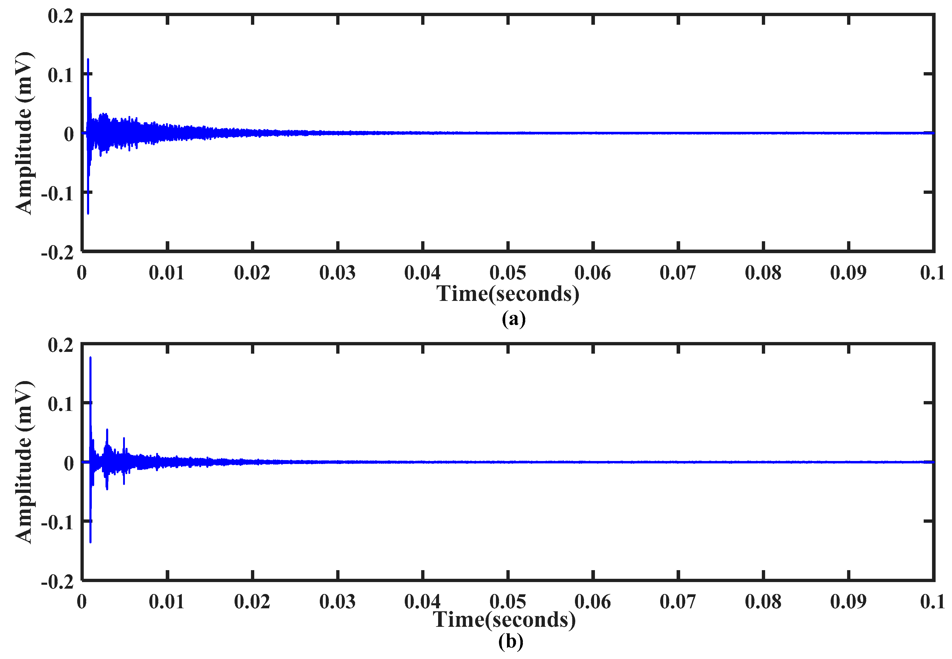
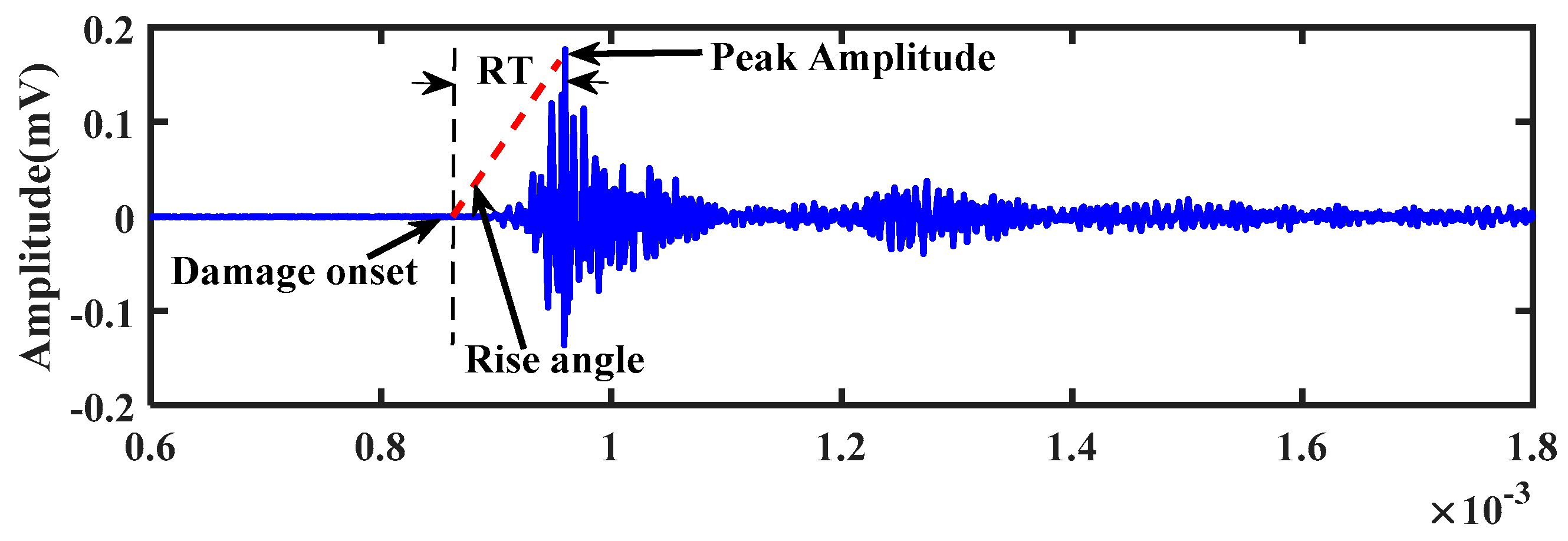
An AE dataset acquired from a spherical storage tank was used in this study to validate the effectiveness of the proposed model. The dataset consists of AE signals collected under two different conditions: Normal and with a 3 mm diameter pinhole crack. The purpose of the experiment is to identify whether each signal belongs to the normal condition or the cracked condition. Figure 7 shows the acoustic signals under the two conditions. To check the presence of the crack, we first analyze the AE signals. The rise angle of the obtained AE signals under the cracked condition was first observed because it was directly affected by the presence of the crack. When a crack develops on the surface of a tank, the effect of the event propagates as an elastic wave. We can observe the activity with the help of rise angle of the AE waveform. In Figure 8, the impact of the AE activity on signal rise angle can be observed. The delay between the onset of damage and the peak amplitude is short, which is termed as high-rise angle caused due to the volumetric change; hence it proves the presence of the crack. As is evident in Figure 7 and Figure 8, classification using raw AE signals in their original form (time-domain values) is not an easy task. Therefore, we extracted the time-domain statistical features from the AE signals. These time-domain statistical features project the AE signals into a reduced features space. The features extraction step is also needed to extract discriminant information from the signals. In the next step, the extracted time-domain statistical features were provided to the support vector machine (SVM) binary classifier. The kernel function used during training and validation of the model was a radial basis (Gaussian) kernel.
To obtain stable experimental results, we used a cross-validation technique. In cross-validation, a sample dataset is uniquely divided into training samples and test samples. Statistically and computationally, it is important to use a cross validation technique. In cross validation, the dataset is divided into subsets. Each subset is used once for testing and times for training.
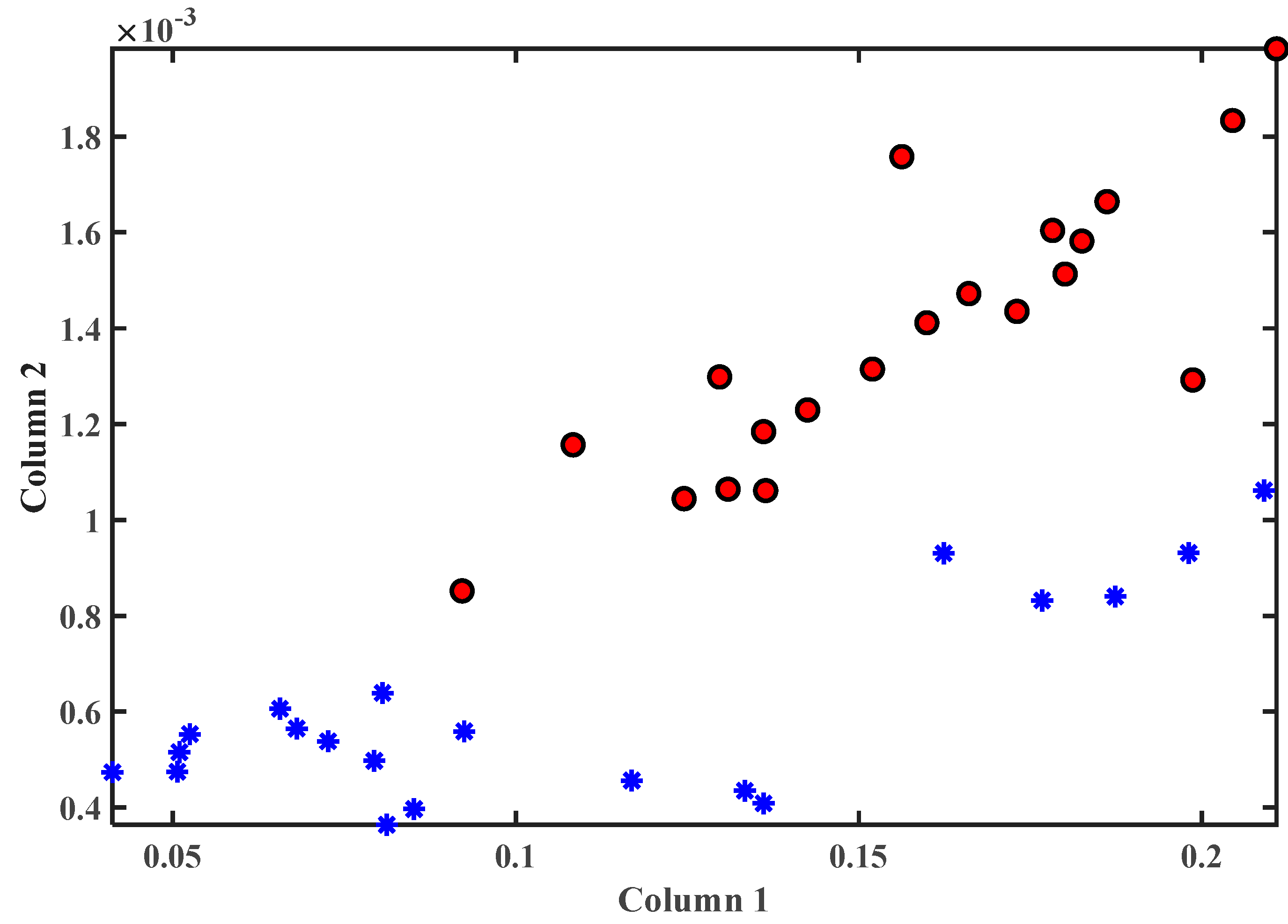
In Figure 9, the feature vectors belonging to the two classes are separated by the SVM decision boundary. The blue samples belong to the normal condition and the red samples belong to the crack condition. It can be observed that the instances of the two classes were well identified and properly separated. Therefore, in turn, the classification accuracy of the developed model was also enhanced.
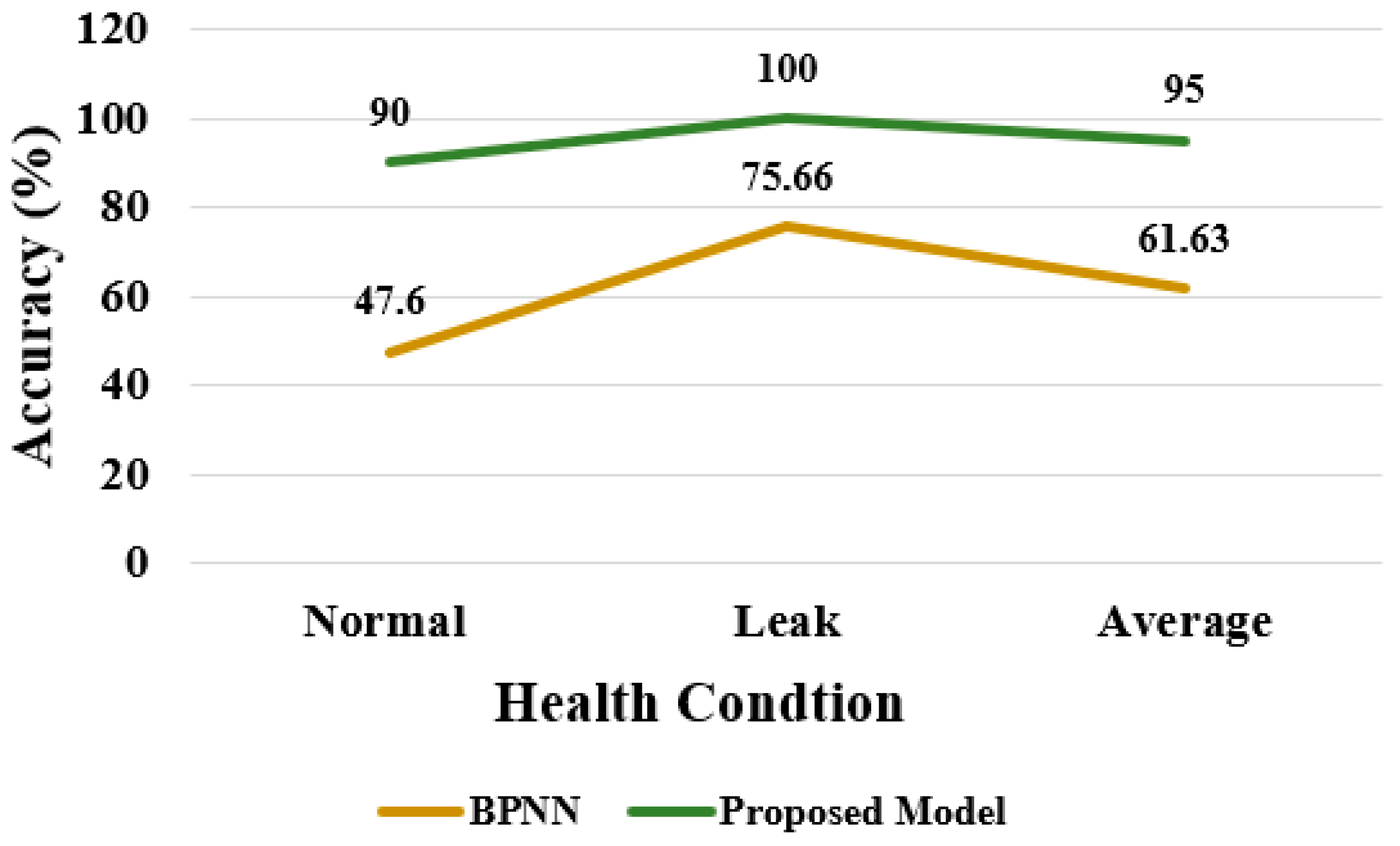
To further verify the effectiveness of the proposed model, we compared the classification results of the proposed model with those of a state-of-the-art machine-learning algorithm, that is, a backpropagation neural network (BPNN) algorithm. A two-layered BPNN was developed with 10 neurons in each layer. We replaced the SVM in the proposed method with the BPNN to create a similar work flow. We used sigmoid activation in the BPNN because the sample dataset was nonlinear. The same set of time-domain statistical features were provided to the BPNNs. We repeated the experiment with the BPNN multiple times to obtain stable results. The results of the proposed model are shown in Figure 10. The average classification accuracy of the proposed model for AE signals acquired from a spherical tank under normal and leak conditions was better than 95%. The model was able to accurately classify instances from the pinhole crack condition: This classification accuracy was 100%. However, under normal conditions, a few instances were misclassified because the time-domain statistical features did not provide enough discriminative information to the subsequent classifier. This means that some of the features in this class overlapped the features of the second class, so the SVM misclassified them. The average classification accuracy of the BPNN was 61.63% for the same experimental setup. The normal-condition classification accuracy was 47.60%, and the fault-condition classification accuracy was 75.66%. This shows that the BPNN was unable to properly differentiate some of the instances into the normal and cracked classes, reducing the average classification accuracy.
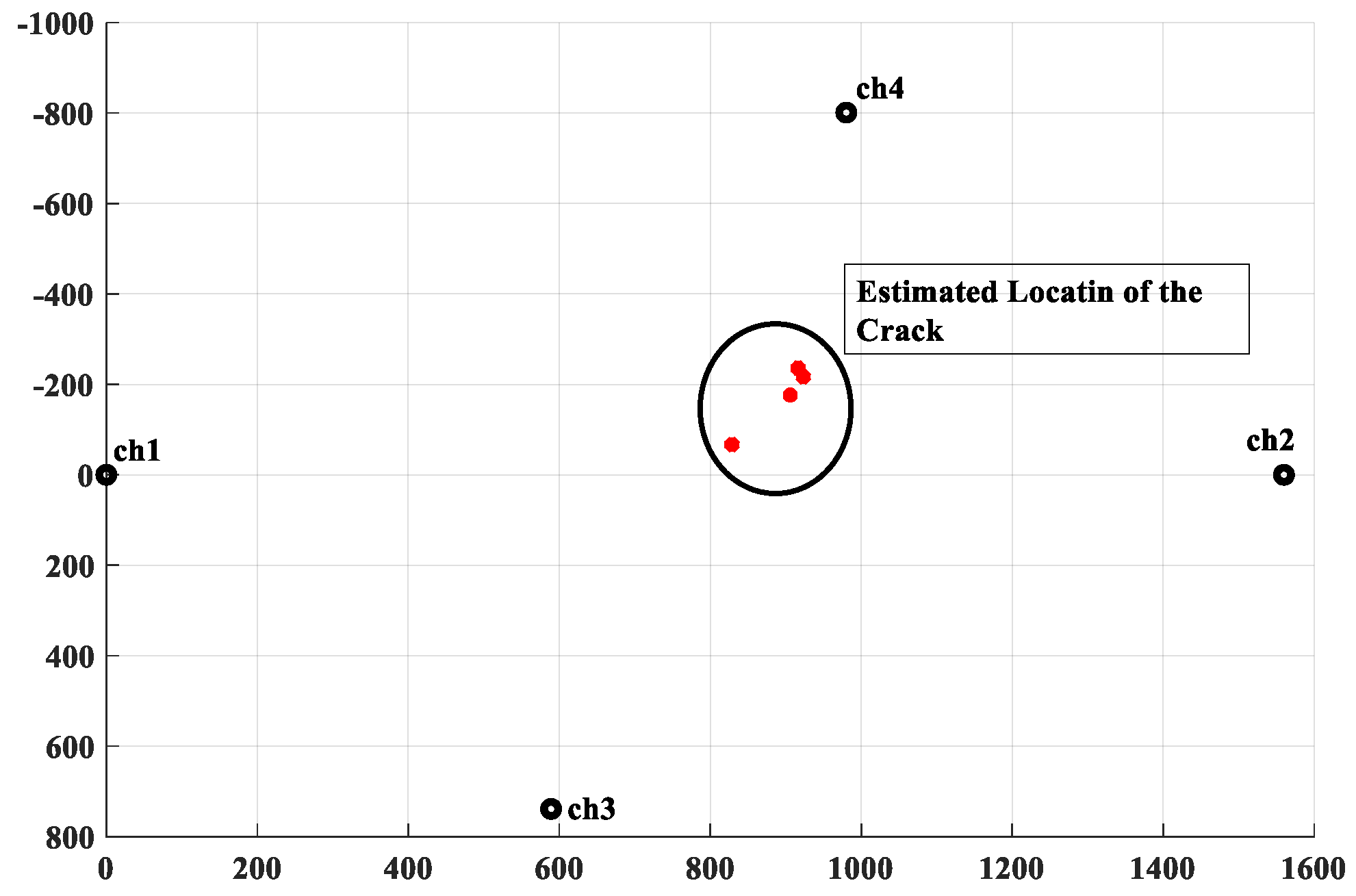
In addition to the classification results, we estimate the crack location in this study. The location of the crack is estimated based on the source localization technique given in [24]. The source can be localized by geometrical arguments by using the following formula:
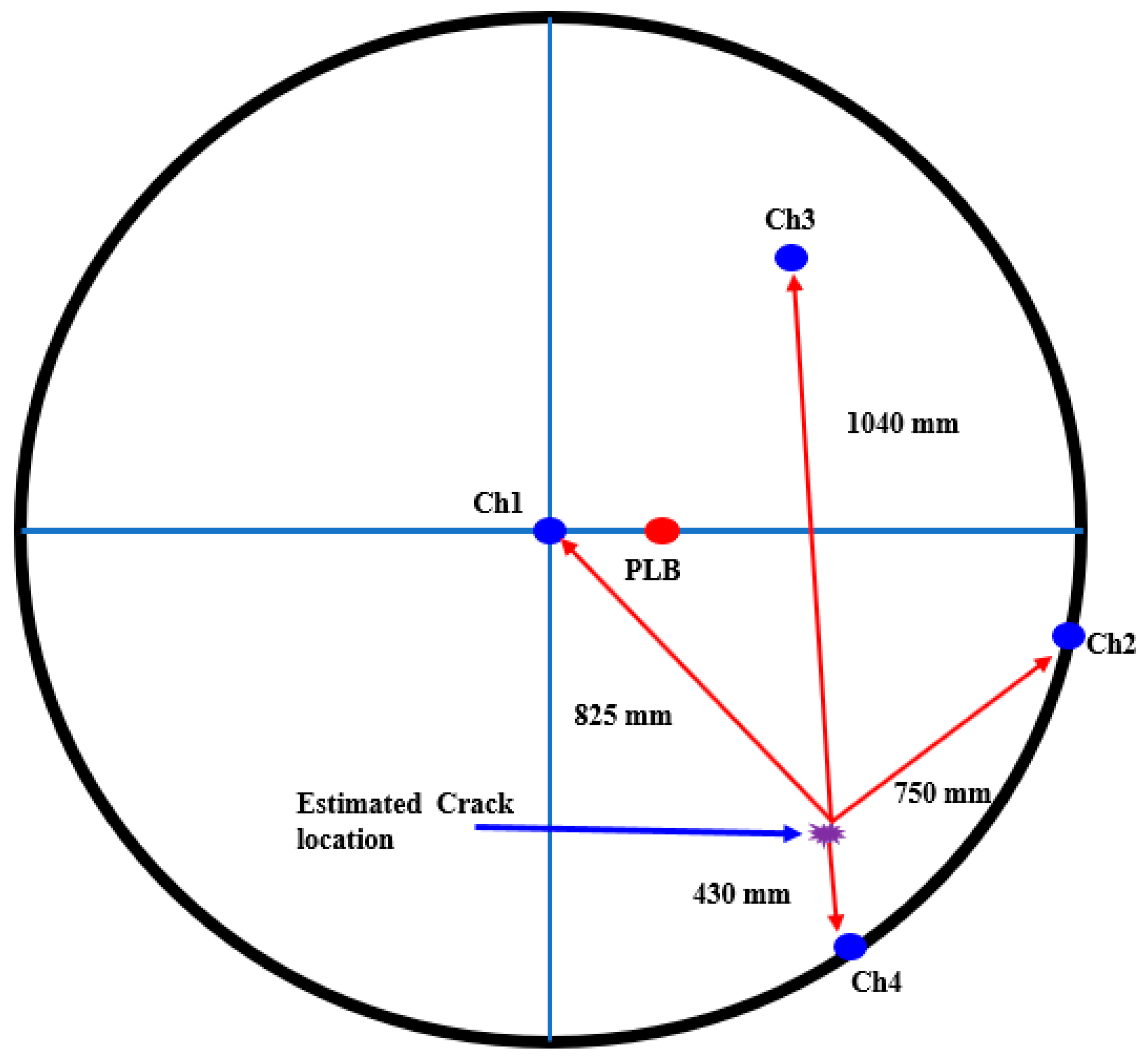
In the above equation, if the position of each sensor is given by and the source location is given by , then the resulting quantity is the desired distance among the source and the sensors. In Figure 11, a planer diagram by using the geometrical relationship of the sensors and the source for our experiment is presented. The red points show the estimated location about the source of origin of the AE signals for the four pencil lead break (PLB) tests. It can be observed that the density of the estimated points was near to the channel 4, and thus it can be assumed that the location of the signals originating from the crack was near to this channel.
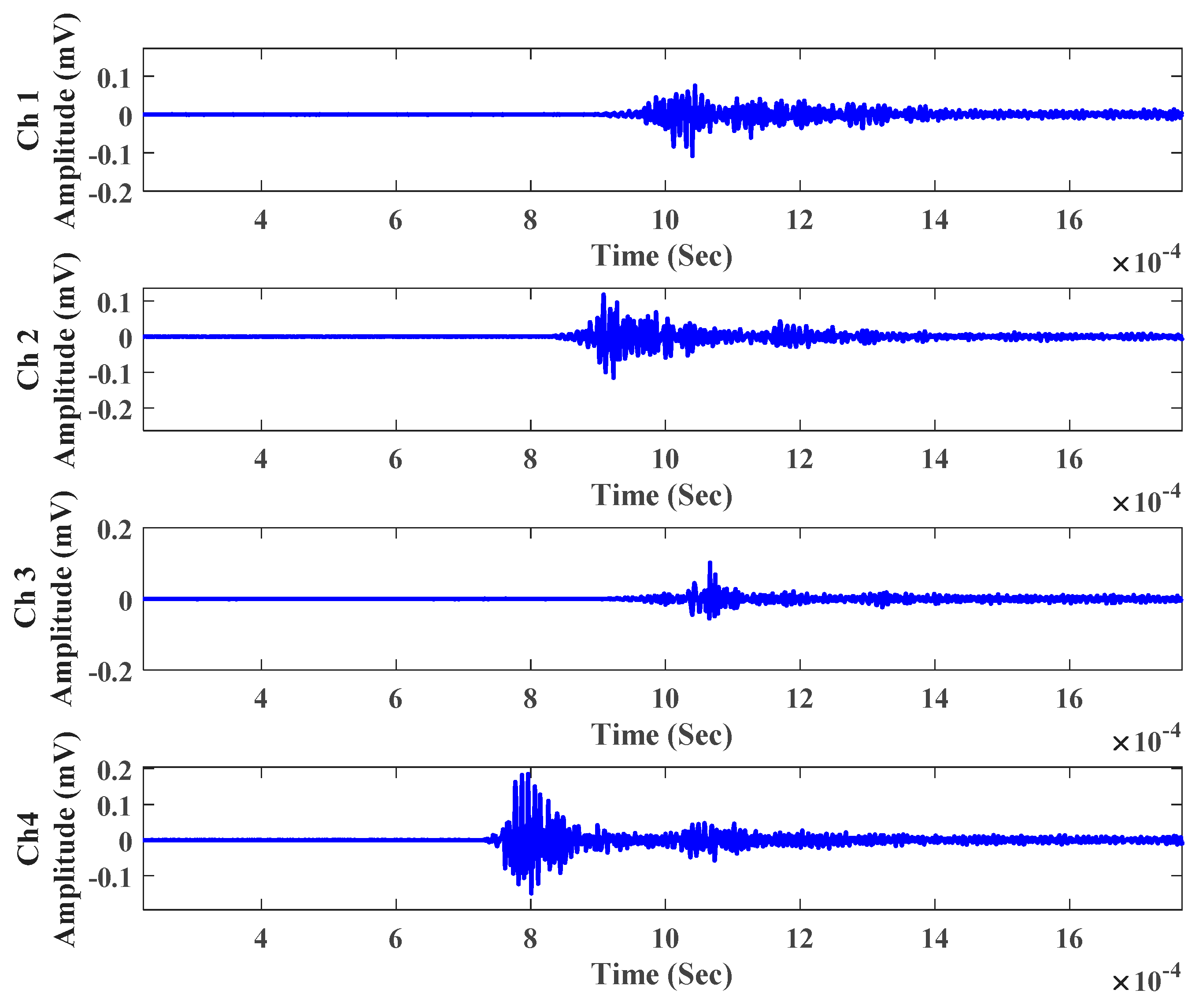
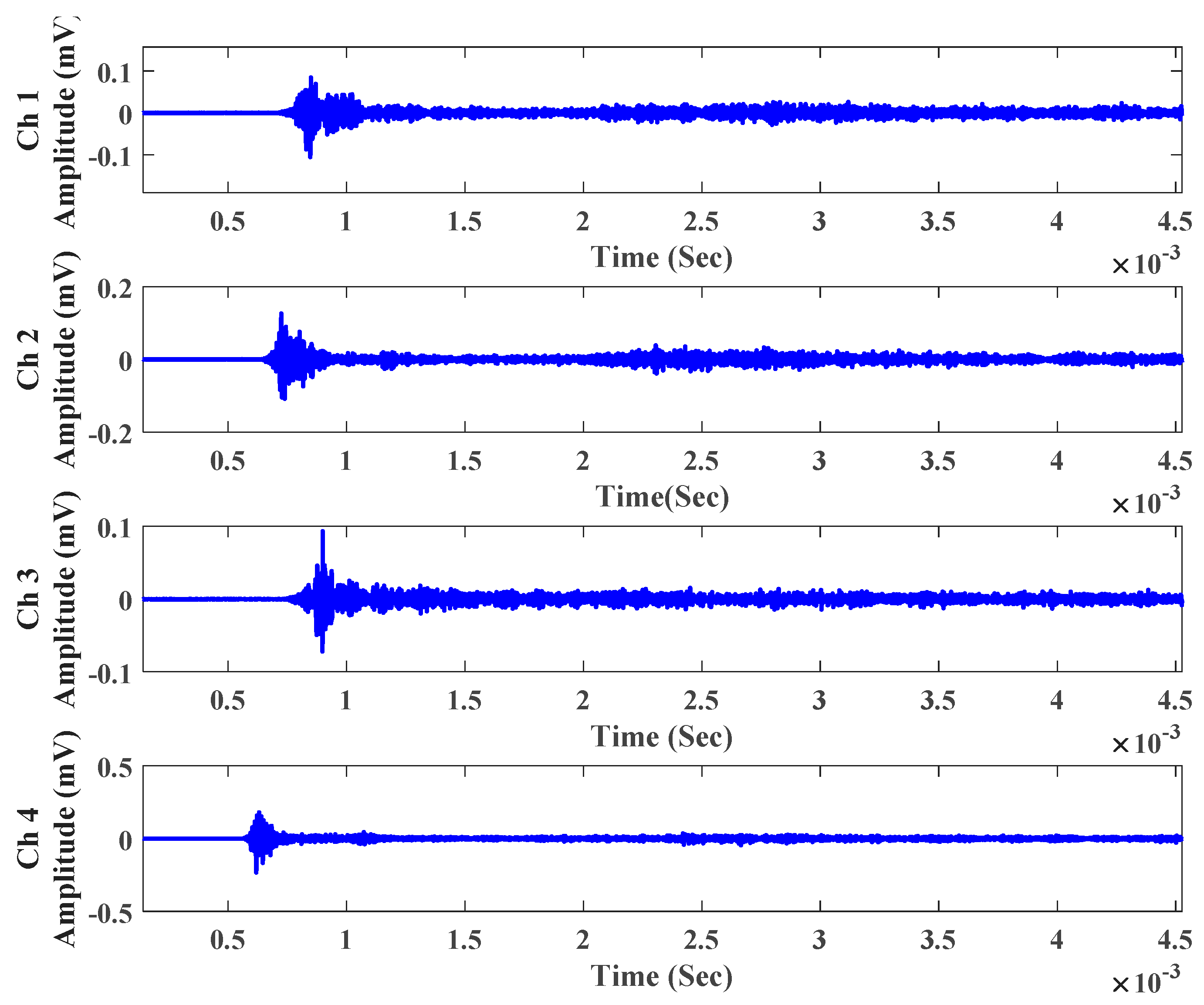
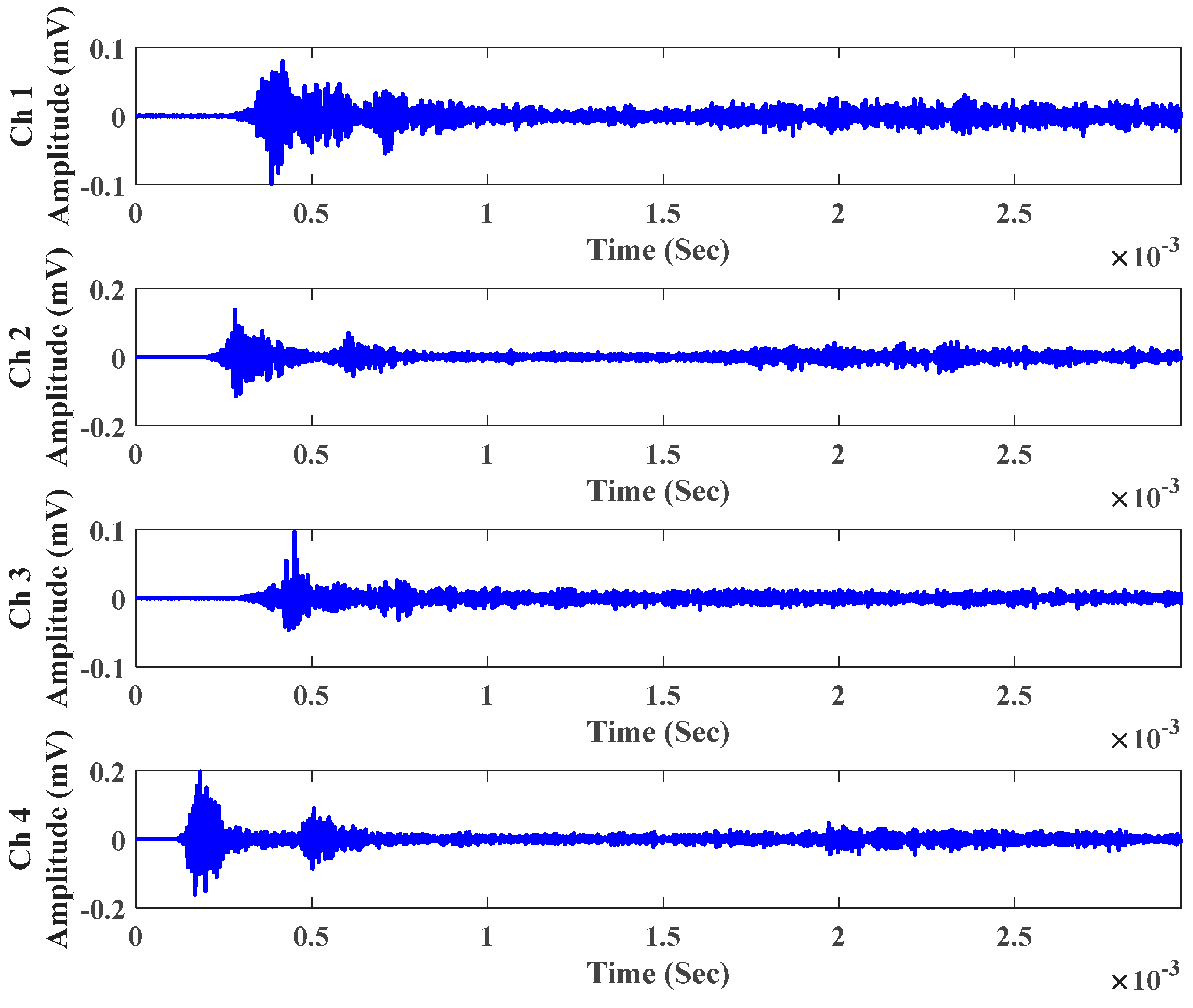
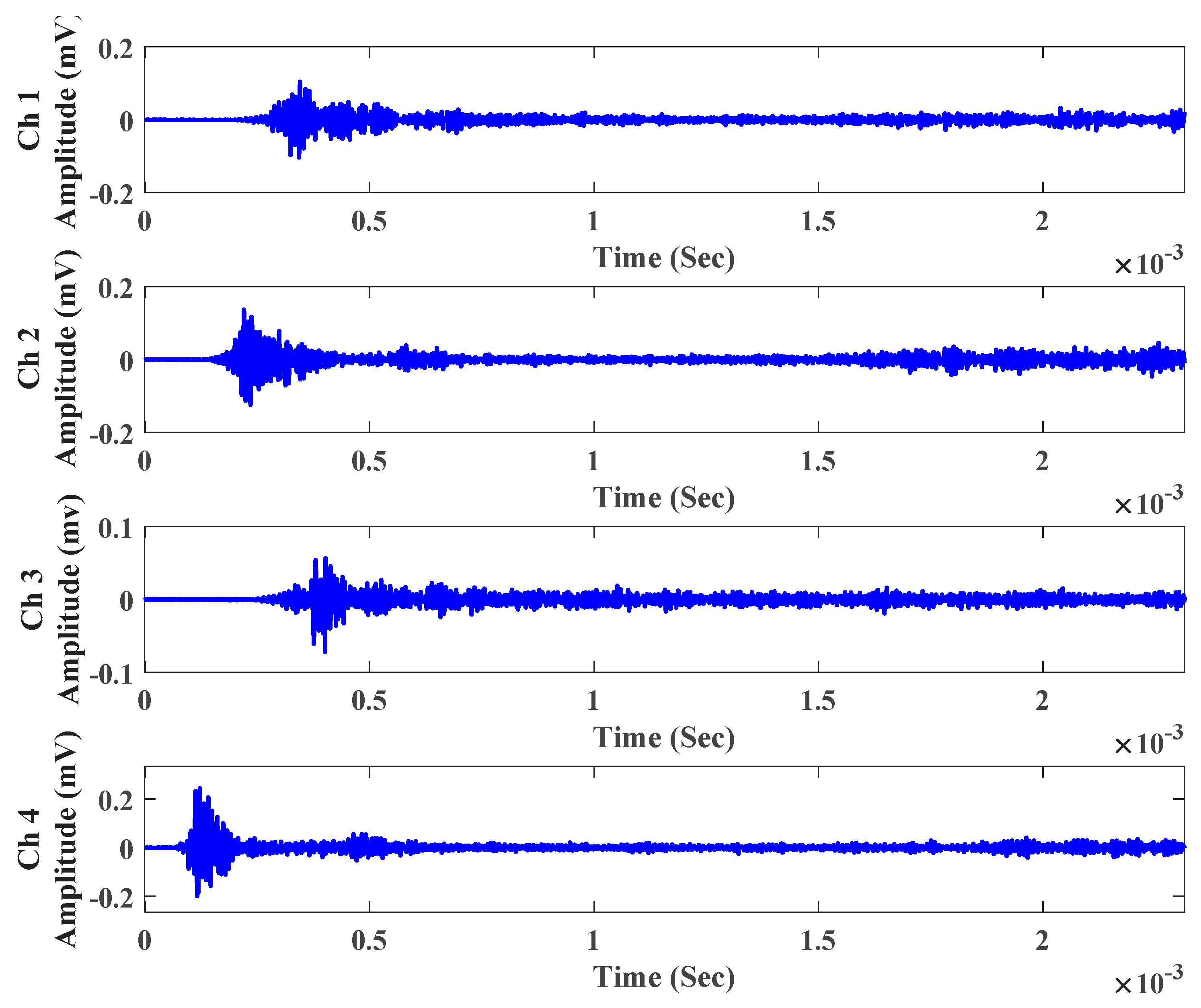
The notion about the estimated source location can be consolidated by analyzing the waveforms of the AE signals obtained during the four PLB tests. Theoretically, the location of the crack was near to the sensor which has minimum arrival time of the signals. The arrival time of a signal to a sensor can be obtained from the signal waveform. In this study, four PLB tests were conducted to excite the crack and get the crack signal. The signals obtained during the four PLB tests are given in Figure 12, Figure 13, Figure 14 and Figure 15. It is evident that in all the four tests, channel 4 first received the signals. We can also observe that channel 2 received the signals a little later as compared to channel 4 and the next one in line was channel 1. In all the tests, channel 3 was the last one to receive the signals, as the time of arrival of the signals was maximum in this case. Another trait worth noticing is that the amplitude of the signals for the channel 4 was grater compared to the signals of the other channels in all the PLB tests. This also indicates that the channel 4 was near to the crack location, as the signals for this channel encountered little attenuation during all the four PLB tests.
Moreover, to further check whether the estimated location of the crack is correct, we calculated the distance of the crack based on time of arrival and velocity of the AE signals for PLB 1. The time of arrival is calculated by using the following expression:
where represents the velocity of the signals, is the distance of a certain sensor from the crack location and is the time of arrival of the signal to the sensor. In this case, the velocity of the AE signal was 3,032,407 mm/s. Moreover, the time of arrival of the signals to the four channels was also known, as presented in Table 4.
By incorporating the velocity and time of arrival information in (7), the location of the leak can be estimated. The estimated distances of the crack from the four channels are given in Figure 16. It is obvious from the figure that the distance between the estimated location of the leak and channel 4 was minimal compared to others. It was also observed that channel 4 received the signal well before the other channels from the time of arrival given in Table 3. Therefore, based on all the information, it can be assumed that the leak was in the vicinity of the channel 4.
5. Conclusions
In this paper, we performed a quantitative assessment of AE signals acquired from a spherical storage tank. The main objective of this work was to perform data-driven structural integrity assessment of a spherical storage tank. We recorded one-second-long AE signals from the test bed under normal (no crack) and cracked (3-mm pinhole crack) conditions. Then, we extracted time-domain statistical features from these AE signals. These features are a compressed representation of the original signals used to differentiate instances into the two classes, as well as to avoid the high computational complexity of the original time-domain signals. The extracted features were then provided to the support vector machine (SVM) classifier. The results showed that the proposed method provides an average accuracy of 90%, making it an effective data classifier. We conclude that the proposed method can be deployed to effectively detect leakage in spherical storage tanks.
Author Contributions
Conceptualization, M.S., D.-C.J., J.-M.K.; Methodology, M.S., M.I., J.K.; Software, M.S.; Validation, M.S. and J.-M.K.; Formal Analysis, M.S. and M.I.; Investigation, M.S., D.-C.J. J.-M.K.; Resources, M.S., M.I., J.K.; Data Curation, M.S., M.I., J.K.; Writing-Original Draft Preparation, M.S.; Writing-Review & Editing, M.I., J.K., D.-C.J., and J.-M.K.; Supervision, J.-M.K.; Funding Acquisition, J.-M.K.
Funding
This work was supported by the Korea Institute of Energy Technology Evaluation and Planning (KETEP) and the Ministry of Trade, Industry & Energy (MOTIE) of the Republic of Korea (No. 20162220100050). This research was also financially supported by the Ministry of SMEs and Startups (MSS), Korea, under the “Regional Specialized Industry Development Program (R&D or non-R&D, P0002964)” supervised by the Korea Institute for Advancement of Technology (KIAT).
Conflicts of Interest
The authors declare no conflicts of interest.
References
- Barker, G. Storage tanks. In The Engineer’s Guide to Plant Layout and Piping Design for the Oil and Gas Industries; Barker, G., Ed.; Gulf Professional Publishing: Houston, TX, USA, 2018; Chapter 15; pp. 361–380. [Google Scholar]
- Luo, T.; Wu, C.; Duan, L. Fishbone diagram and risk matrix analysis method and its application in safety assessment of natural gas spherical tank. J. Clean. Prod. 2018, 174, 296–304. [Google Scholar] [CrossRef]
- Kennedy, M.S.; Moegling, S.; Sarikelle, S.; Suravallop, K. Assessing the effects of storage tank design on water quality. J. Am. Water Works Assoc. 1993, 85, 78–88. [Google Scholar] [CrossRef]
- Wilson, S.; Zhang, H.; Burwell, K.; Samantapudi, A.; Dalemarre, L.; Jiang, C.; Rice, L.; Williams, E.; Naney, C. Leaking Underground Storage Tanks and Environmental Injustice: Is There a Hidden and Unequal Threat to Public Health in South Carolina? Environ. Justice 2013, 6, 175–182. [Google Scholar] [CrossRef] [PubMed] [Green Version]
- Gholizadeh, S. A review of non-destructive testing methods of composite materials. Procedia Struct. Integr. 2016, 1, 50–57. [Google Scholar] [CrossRef] [Green Version]
- Blitz, J. Electrical and Magnetic Methods of Non-Destructive Testing; Springer Science & Business Media: Berlin, Germany, 2012; Volume 3. [Google Scholar]
- Guyott, C.C.H.; Cawley, P.; Adams, R.D. The Non-destructive Testing of Adhesively Bonded Structure: A Review. J. Adhes. 1986, 20, 129–159. [Google Scholar] [CrossRef]
- Pollock, A.A. Acoustic emission—2: Acoustic emission amplitudes. Non-Destr. Test. 1973, 6, 264–269. [Google Scholar] [CrossRef]
- Niccolini, G.; Durin, G.; Carpinteri, A.; Lacidogna, G.; Manuello, A. Crackling noise and universality in fracture systems. J. Stat. Mech. Theory Exp. 2009, 2009, P01023. [Google Scholar] [CrossRef]
- Bontea, D.-M.; Chung, D.; Lee, G. Damage in carbon fiber-reinforced concrete, monitored by electrical resistance measurement. Cem. Concr. Res. 2000, 30, 651–659. [Google Scholar] [CrossRef]
- Niccolini, G.; Borla, O.; Accornero, F.; Lacidogna, G.; Carpinteri, A. Scaling in damage by electrical resistance measurements: An application to the terracotta statues of the Sacred Mountain of Varallo Renaissance Complex (Italy). Rendiconti Lincei 2015, 26, 203–209. [Google Scholar] [CrossRef]
- Zongjin, L.; Surendra, P.S. Localization of Microcracking in Concrete Under Uniaxial Tension. Mater. J. 1994, 91, 372–381. [Google Scholar]
- Morofuji, K.; Tsui, N.; Yamada, M.; Maie, A.; Yuyama, S.; Li, Z. Quantitative study of acoustic emission due to leaks from water tanks. System 2003, 5, 213–222. [Google Scholar]
- Li, W.; Dai, G.; Wang, Y.; Long, F. Study of Tank Acoustic Emission Testing Signals Analysis Method Based on Wavelet Neural Network. In Proceedings of the ASME 2011 Pressure Vessels and Piping Conference, Baltimore, MD, USA, 17–21 July 2011; American Society of Mechanical Engineers: New York, NY, USA, 2011; pp. 699–703. [Google Scholar]
- Hasan, M.J.; Sohaib, M.; Kim, J.-M. 1D CNN-Based Transfer Learning Model for Bearing Fault Diagnosis under Variable Working Conditions; Springer International Publishing: Cham, Switzerland, 2019; pp. 13–23. [Google Scholar]
- Pratondo, A.; Chui, C.-K.; Ong, S.-H. Integrating machine learning with region-based active contour models in medical image segmentation. J. Vis. Commun. Image Represent. 2017, 43, 1–9. [Google Scholar] [CrossRef]
- Arganda-Carreras, I.; Kaynig, V.; Rueden, C.; Eliceiri, K.W.; Schindelin, J.; Cardona, A.; Sebastian Seung, H. Trainable Weka Segmentation: A machine learning tool for microscopy pixel classification. Bioinformatics 2017, 33, 2424–2426. [Google Scholar] [CrossRef] [PubMed]
- Goldberg, Y. Neural network methods for natural language processing. Synth. Lect. Hum. Lang. Technol. 2017, 10, 1–309. [Google Scholar] [CrossRef]
- Zhang, Y.; Chan, W.; Jaitly, N. Very deep convolutional networks for end-to-end speech recognition. In Proceedings of the 2017 IEEE International Conference on Acoustics, Speech and Signal Processing (ICASSP), New Orleans, LA, USA, 5–9 March 2017; IEEE: New York, NY, USA, 2017; pp. 4845–4849. [Google Scholar] [Green Version]
- Tra, V.; Kim, J.; Khan, S.A.; Kim, J.-M. Bearing Fault Diagnosis under Variable Speed Using Convolutional Neural Networks and the Stochastic Diagonal Levenberg-Marquardt Algorithm. Sensors 2017, 17, 2834. [Google Scholar] [CrossRef] [PubMed]
- Sohaib, M.; Kim, C.-H.; Kim, J.-M. A Hybrid Feature Model and Deep-Learning-Based Bearing Fault Diagnosis. Sensors 2017, 17, 2876. [Google Scholar] [CrossRef] [PubMed]
- Cristianini, N.; Shawe-Taylor, J. An Introduction to Support Vector Machines and Other Kernel-Based Learning Methods; Cambridge University Press: Cambridge, UK, 2000. [Google Scholar]
- American Society of Mechanical Engineers. Boiler and Pressure Vessel Code; American Society of Mechanical Engineers: New York, NY, USA, 2004. [Google Scholar]
- Salinas, V.; Vargas, Y.; Ruzzante, J.; Gaete, L. Localization algorithm for acoustic emission. Phys. Procedia 2010, 3, 863–871. [Google Scholar] [CrossRef] [Green Version]
Figure 1.
The proposed spherical tank crack-detection model. AE: acoustic emissions.

Figure 2.
A hyperplane separating two linearly separable classes.

Figure 3.
SVM demo for separating two nonlinearly separable classes via a hyperplane by using a Gaussian kernel function.
Figure 3.
SVM demo for separating two nonlinearly separable classes via a hyperplane by using a Gaussian kernel function.

Figure 4.
Testbed used to collect acoustic emissions in the experiment.

Figure 5.
Schematic representation of the testbed.

Figure 6.
The data acquisition system. PC: personal computer; PCI: peripheral component interconnect; WDI-AST: wideband differential; AE sensor.
Figure 6.
The data acquisition system. PC: personal computer; PCI: peripheral component interconnect; WDI-AST: wideband differential; AE sensor.

Figure 7.
(a) Normal acoustic emission signals from the spherical tank; (b) Acoustic emission signals from the spherical tank with a 3 mm pinhole crack.
Figure 7.
(a) Normal acoustic emission signals from the spherical tank; (b) Acoustic emission signals from the spherical tank with a 3 mm pinhole crack.

Figure 8.
The rise angle produced due the crack development on the spherical tank.

Figure 9.
SVM boundary line identification around the two feature vectors of the two classes. The blue samples belong to the normal condition and the red samples belong to the crack condition.
Figure 9.
SVM boundary line identification around the two feature vectors of the two classes. The blue samples belong to the normal condition and the red samples belong to the crack condition.

Figure 10.
Classification accuracy comparison of the proposed spherical tank leakage detection model with a back propagation neural network.
Figure 10.
Classification accuracy comparison of the proposed spherical tank leakage detection model with a back propagation neural network.

Figure 11.
Planer diagram of the estimated location of the crack.

Figure 12.
Acoustic emission signals obtained from the pencil lead break test (PLB) 1.

Figure 13.
Acoustic emission signals obtained from the pencil lead break test (PLB) 2.

Figure 14.
Acoustic emission signals obtained from the pencil lead break test (PLB) 3.

Figure 15.
Acoustic emission signals obtained from the pencil lead break test (PLB) 4.

Figure 16.
Crack position estimation through the velocity and time of arrival technique.


Table 1.
Statistical time domain features (x is the acoustic emission signal).
| Features | Expression | Features | Expression | Features | Expression |
|---|---|---|---|---|---|
| Peak (P) | Root mean square (RMS) | Crest factor (Cf) | |||
| Impulse factor (IF) | Kurtosis (K) | Skewness(S) | |||
| Square root Me an (SRM) | Margin factor (MF) | Peak-to-peak value (PP) | |||
| Kurtosis factor (KF) | Energy (E) | Shape factor (SF) | |||
| Clearance Factor (CF) |
Table 2.
Experimental setup details. PCI: peripheral component interconnect; WDI-AST: wideband differential; AE sensor.
Table 2.
Experimental setup details. PCI: peripheral component interconnect; WDI-AST: wideband differential; AE sensor.
| Acoustic Emission sensor (WDI-AST sensor) | Peak sensitivity (V/ms); [V/μbar]: 96[–25 dB] Operating frequency range: 200 to 900 kHz Directionality: ±1.5 d BResonant frequency: 650 kHz |
| PCI board with 2-channel AE sensor | 18-bit 40 MHz A/D conversion AE input: 2 channels (one is 10 M samples/s rate, and another is 5 M samples/s as two channels, with simultaneously used) |
Table 3.
Dataset description.
| Signal Type | Fault Location | Pinhole Size (mm) | Percentage of Training Samples | Percentage of Test Samples | Number of Channels |
|---|---|---|---|---|---|
| Normal | None | 0 | 60 | 40 | 4 |
| Pinhole crack | Bottom of the tank | 3 | 60 | 40 |
Table 4.
Time of arrival of the AE signals for four channels (sensors).
| Channel Number (Sensor) | Time of Arrival (milli-seconds) |
|---|---|
| 1 | 0.27 |
| 2 | 0.24 |
| 3 | 0.34 |
| 4 | 0.14 |
© 2019 by the authors. Licensee MDPI, Basel, Switzerland. This article is an open access article distributed under the terms and conditions of the Creative Commons Attribution (CC BY) license (http://creativecommons.org/licenses/by/4.0/).
Share and Cite
MDPI and ACS Style
Sohaib, M.; Islam, M.; Kim, J.; Jeon, D.-C.; Kim, J.-M. Leakage Detection of a Spherical Water Storage Tank in a Chemical Industry Using Acoustic Emissions. Appl. Sci. 2019, 9, 196. https://0-doi-org.brum.beds.ac.uk/10.3390/app9010196
AMA Style
Sohaib M, Islam M, Kim J, Jeon D-C, Kim J-M. Leakage Detection of a Spherical Water Storage Tank in a Chemical Industry Using Acoustic Emissions. Applied Sciences. 2019; 9(1):196. https://0-doi-org.brum.beds.ac.uk/10.3390/app9010196
Chicago/Turabian StyleSohaib, Muhammad, Manjurul Islam, Jaeyoung Kim, Duck-Chan Jeon, and Jong-Myon Kim. 2019. "Leakage Detection of a Spherical Water Storage Tank in a Chemical Industry Using Acoustic Emissions" Applied Sciences 9, no. 1: 196. https://0-doi-org.brum.beds.ac.uk/10.3390/app9010196
Note that from the first issue of 2016, this journal uses article numbers instead of page numbers. See further details here.