Landslide Susceptibility Mapping Based on Random Forest and Boosted Regression Tree Models, and a Comparison of Their Performance

Abstract

This study aims to analyze and compare landslide susceptibility at Woomyeon Mountain, South Korea, based on the random forest (RF) model and the boosted regression tree (BRT) model. Through the construction of a landslide inventory map, 140 landslide locations were found. Among these, 42 (30%) were reserved to validate the model after 98 (70%) had been selected at random for model training. Fourteen landslide explanatory variables related to topography, hydrology, and forestry factors were considered and selected, based on the results of information gain for the modeling. The results were evaluated and compared using the receiver operating characteristic curve and statistical indices. The analysis showed that the RF model was better than the BRT model. The RF model yielded higher specificity, overall accuracy, and kappa index than the BRT model. In addition, the RF model, with a prediction rate of 0.865, performed slightly better than the BRT model, which had a prediction rate of 0.851. These results indicate that the landslide susceptibility maps (LSMs) produced in this study had good performance for predicting the spatial landslide distribution in the study area. These LSMs could be helpful for establishing mitigation strategies and for land use planning.

1. Introduction

A landslide is defined as a natural disaster that occurs when gravity causes a mass of debris, soil, or rock to move on a downward slope [1]. The majority of landslides occur as a result of hydroclimatic events, such as prolonged or intensive rain. Furthermore, mechanisms such as seismic triggers, wind, and freeze–thaw cycles are known to initiate landslides [2].

Mountains with shallow layers of soil that have formed in place from weathered gneiss and granite make up roughly 70% of the Korean peninsula [3]. Such terrain is vulnerable to weakening during heavy rainfall. Most of the annual precipitation occurs during the summer, when heavy rain and typhoons frequently occur. In particular, the heavy rain associated with typhoons has the potential to cause landslides in South Korea [4]. The year 2011 was a particularly devastating year, with 43 landslide-related casualties in Chuncheon and at Woomyeon Mountain in the area surrounding Seoul City. This is the largest number of landslide-related casualties since 2000.

South Korea has not been alone in experiencing an increase in such natural disasters. Other regions around the world have also experienced more frequent landslides on a larger scale and with more severe damage. In future decades, this trend will probably continue because of ongoing deforestation, increased urbanization, and an increase in regional precipitation in landslide-prone areas due to climate change [5]. It is essential that both susceptible and stable areas be identified to mitigate property damage, environmental degradation, and loss of life. Consequently, landslide susceptibility assessments, i.e., assessments of the spatial probability of a landslide occurring, are a huge step forward in the comprehensive hazard management of landslides [6,7]. The landslide susceptibility map (LSM) produced by a landslide susceptibility assessment can be a useful tool for authorities with decision-making capabilities.

Many methods and techniques have been proposed to evaluate landslide susceptibility. In the past few decades, statistical approaches have become popular in the use of remote sensing (RS) with a geographic information system (GIS). There are many statistical approaches used in landslide susceptibility assessment, including a frequency ratio (FR) [8,9], certainty factor (CF) [10], statistical index (SI) [11,12], as well as weight of evidence (WoE) [7,13,14] and logistic regression (LR) [15,16] approaches.

Recently, machine learning techniques have become popular in various fields. Machine learning, a branch of artificial intelligence, uses computer algorithms to analyze and predict information based on learning from training data [17,18]. Due to its robustness and high generalization capability, the use of machine learning has increased in landslide susceptibility analysis. Among the machine learning methods, artificial neural network [19,20], fuzzy logic [21,22], neuro-fuzzy [23], support vector machine [24,25], random forest [26,27], and naïve Bayes tree [17,28] methods have been popularly applied.

More recently, ensemble machine learning techniques have been used to enhance the prediction power and robustness of landslide susceptibility assessment. The ensemble methods, formed by a combination of variously based classifiers, have typically demonstrated significant improvement [17,24,29,30]. Ensemble techniques, which are relatively new approaches for producing a landslide susceptibility map, have been rarely used in the field. Therefore, the main objective of this research was to analyze and compare the performance of different ensemble models—namely, the random forest (RF) and boosted regression tree (BRT) models—for landslide susceptibility analysis. The RF and BRT models are very popular ensemble methods. Both are tree-based algorithms that predict the results by combining individual trees. However, the RF and BRT models build trees in different ways. Considering these characteristics, these models are appropriate for producing LSMs and for comparing LSM results. The results of the models were compared using the receiver operating characteristic (ROC) curve and statistical indices to determine the more robust model.

2. Study Area and Data Used

2.1. Study Area

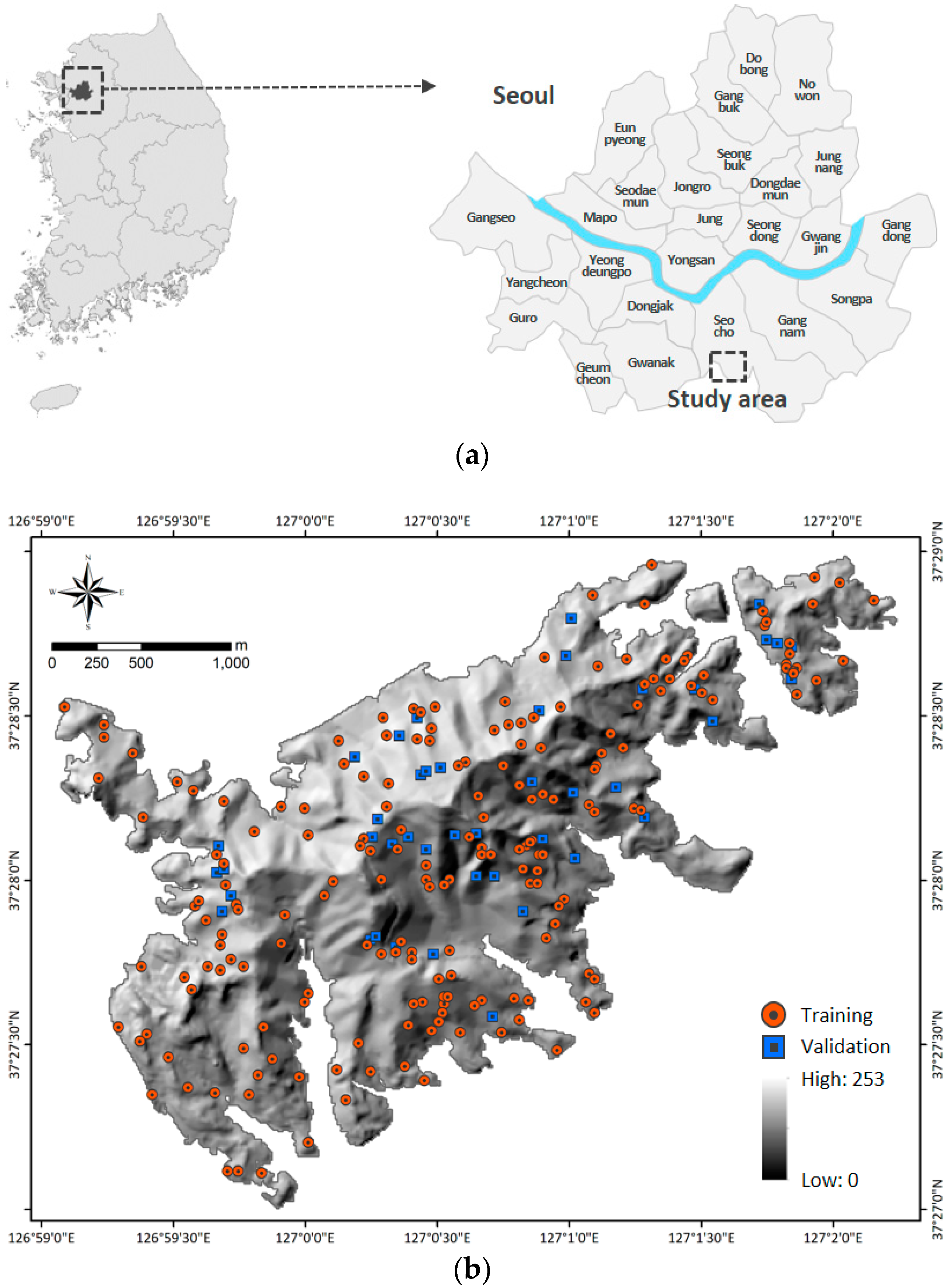
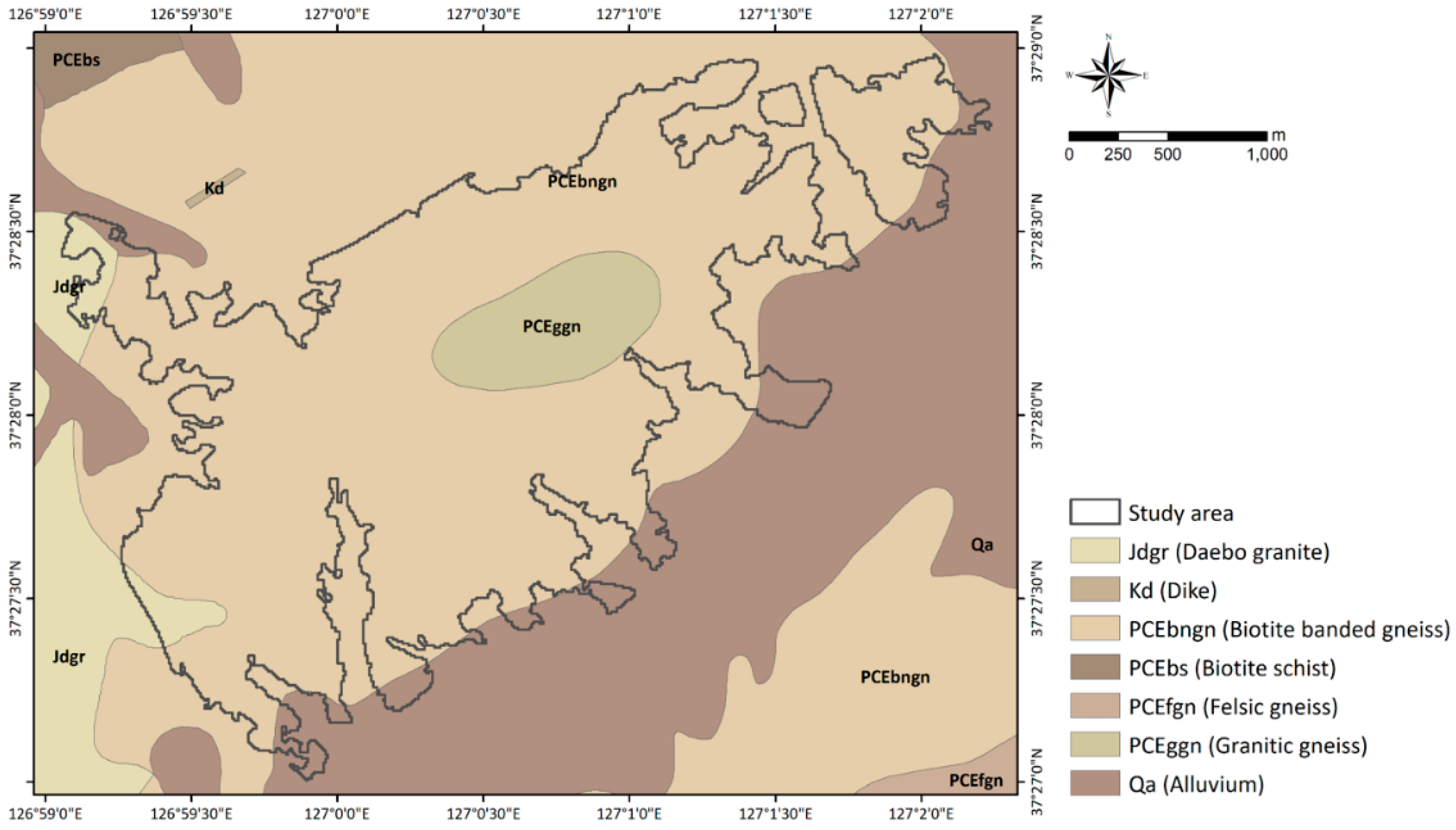
The study area, Woomyeon Mountain, is located in the Seocho district of Seoul City, South Korea. This area lies within 37°27′00″–37°28′55″ N and 126°59′02″–127°01′41″ E (Figure 1). The average elevation is 293 m above sea level, and the slope is approximately 30°–35°. The bedrock is Precambrian banded biotite gneiss, which is believed to be highly susceptible to landslides because of severe weathering and abundant faults (Figure A1). In addition, granite gneiss with relatively poor compositional differentiation is excavated en masse, and there is partial distribution of an embedded dike. The gneiss outcrop is poor, as a result of severe weathering in the overall area, and its foliation structure is irregular, due to several folding events [31].

This area experienced concentrated precipitation from 26–29 July 2011. The maximum precipitation, which occurred during 2 h one morning, was 164 mm. This exceeded the 156-mm, 100-year return period. This heavy precipitation led to a debris flow landslide in the area near Woomyeon Mountain, and 1–1.5 m of stratum flowed over areas near the mountain. Seven locations in the study area, including two locations in the valley area damaged primarily from flooding and five locations damaged by debris flow, were affected by the landslide. The total area damaged by the debris was approximately 276,683 m², and the maximum length of damage from the upper part of the steep-slope disaster area to diffuse areas was approximately 764 m. The event caused 16 deaths and 10 building collapses [31].

2.2. Landslide Inventory

Landslide locations were identified using 32 aerial photographs of the study area, taken after the occurrence of the landslides. These aerial photographs were taken by a digital mapping camera with a spatial resolution of 10 cm. The orthorectified photographs were produced using the Leica Photogrammetry Suite (LPS) mounted on ERDAS Imagine 2011 (Erdas, Inc., Norcross, GA, United States). Landslide locations were digitized by visual interpretation using ArcGIS 10.2 (ESRI, Inc., Redlands, CA, USA). Among the digitized landslide locations, landslide locations belonging to rupture zones were converted to point data using a centroid technique. The point data representing the landslide locations were converted to a pixel format, with resolution of 10 m. From the 140 identified landslides, 42 (30%) were reserved to validate the model, after 98 (70%) had been chosen at random for model training. Additionally, non-landslide pixels were selected randomly from the non-landslide area: 98 non-landslide pixels were used for the training dataset, and 42 non-landslide pixels were used to build the validation dataset. This generating and splitting process was performed repeatedly more than 10 times. Finally, the combination utilized was found through the area under the receiver operating characteristic (ROC) curve (AUC) method.

2.3. Landslide Explanatory Variables

Landslides usually occur by complex interactions among various explanatory variables, and there is no consensus about which landslide explanatory variables to use. In this study, 14 explanatory variables were selected, based on a literature review and data availability. These factors were divided into the following three categories: topography, hydrology, and forestry (

Table 1. Information and sources of data used for the landslide susceptibility assessment at Woomyeon Mountain.

Category	Factor	Source	Scale (Resolution)	GIS and Data Type
-	Landslide inventory	Aerial photographs	1:5000	Raster
Topography	Altitude	Topographic maps	1:5000	Vector
	Slope degree	Digital elevation map	10 × 10 m	Raster
	Slope aspect
	Profile curvature
	Plan curvature
Hydrology	Distance to streams	Digital elevation map	10 × 10 m	Raster
	Topographic wetness index
	Stream power index
	Sediment transport index
	Terrain roughness index
Forestry	Timber type	Forest map	1:5000	Vector
	Timber diameter
	Timber age
	Timber density

, Figure A2). These factors were produced in raster format with a cell size of 10 × 10 m, considering the scale of the input data, using ArcGIS 10.2 and ERDAS Imagine 2011; the total number of cells in the study area was 67,005. For the next process, the continuous variables among the explanatory variables were reclassified into seven classes, using ArcGIS 10.2. ArcGIS 10.2 provides various classification schemes, such as equal interval, standard deviation, natural break, quantile, etc. Natural break classification groups the classes based on break points that are relatively large jumps in data values. This classification method can be used to maximize the variance between classes. In addition, Cao et al. (2016) [32] indicated that natural break classification is more appropriate for the classification of variables, because their results showed that the LSM produced had higher accuracy compared to that using a different classification method. Therefore, natural break classification was used in this study.

2.3.1. Topography Factors

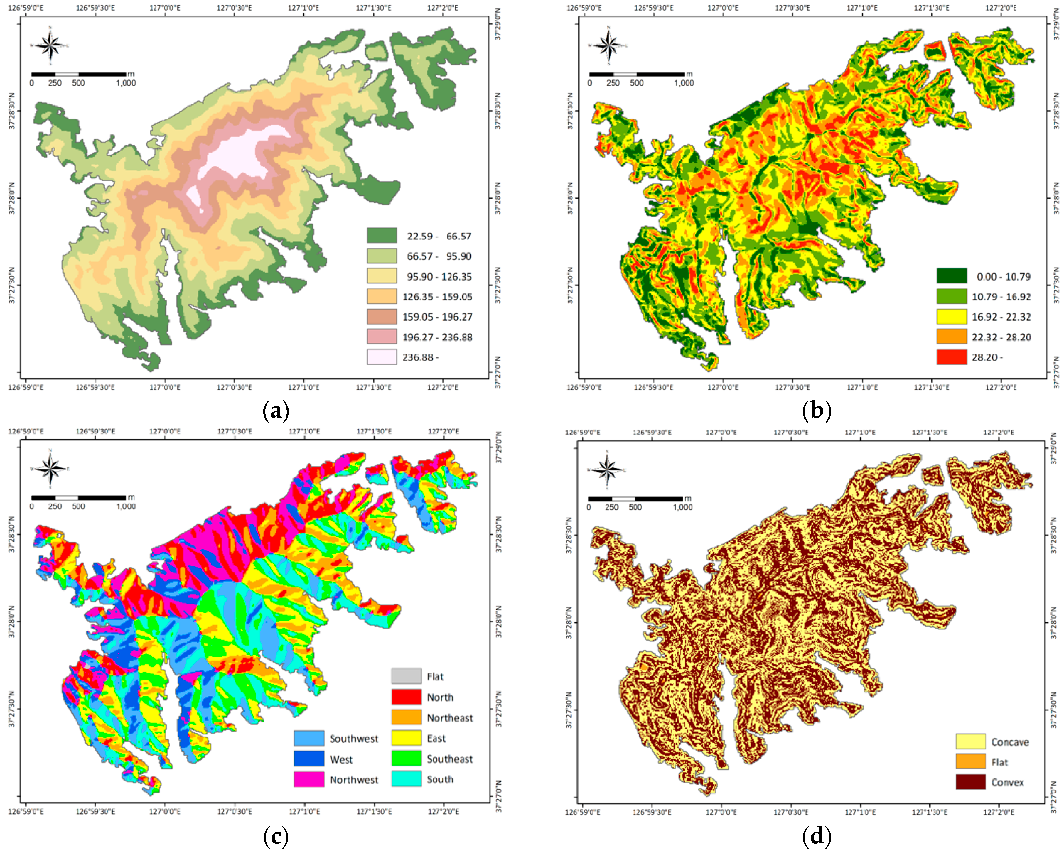
Topography factors include altitude, slope degree, slope aspect, profile curvature, and plan curvature. Altitude is an influential factor among the various landslide explanatory variables, because it is affected by several geomorphologic and geological processes. Slope, which can be described as the form between any section of the surface and a horizontal datum, has considerable influence on slope stability [33]. The degree of vulnerability to landslides may differ based on slope direction, because the water content of the surface, vegetation type, and soil strength may be different. In addition, both the profile and plan curvatures can be classified as flat, concave, or convex. During the rainy season, concave slopes may contain more moisture than convex slopes or flat slopes, so the concave slopes may be more vulnerable to landslides. All of these variables were extracted from the 10-m digital elevation model (DEM), using the spatial analyst tool of ArcGIS. The DEM was produced from 1:5000 topographic maps provided by the Korean National Geographic Information Institute.

2.3.2. Hydrology Factors

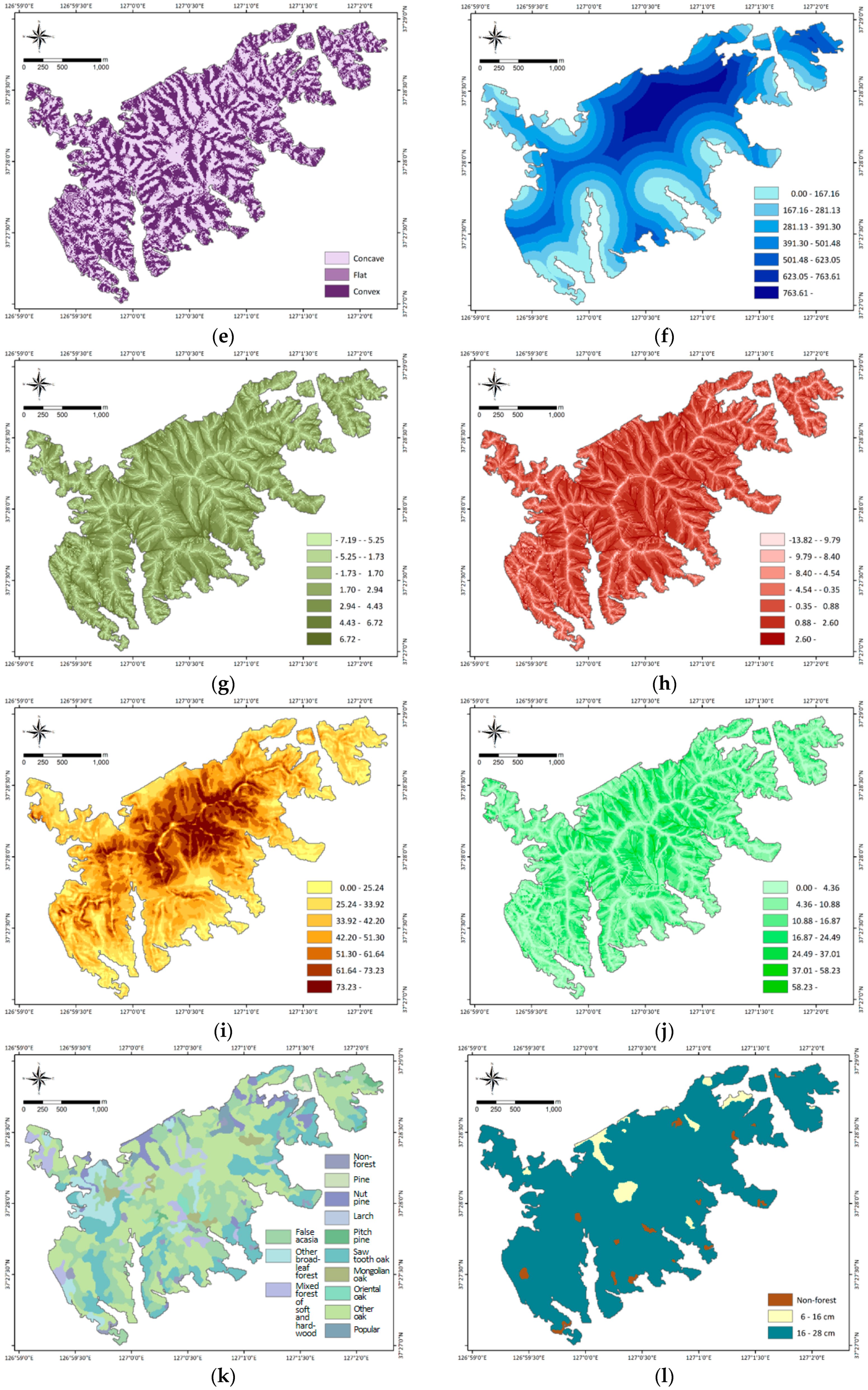
The hydrology factors were distance to streams, topographic wetness index (TWI), stream power index (SPI), sediment transport index (STI), and terrain roughness index (TRI). The streams were delineated by flow accumulation and converted to a vector format. The distance to streams was calculated using the Euclidean distance function in ArcGIS. Beven and Kirby (1979) [34] developed a TWI that reflects water’s tendency to accumulate anywhere within the catchment area, accumulations that will then tend to move downslope as a result of gravity [35]. The water flow’s power to erode is measured by the SPI, based on the assumption of proportionality of discharge to a catchment’s specific area [36]. The STI is also often used to reflect the overland flow’s power to erode [37]. The TWI, SPI, and STI were calculated with their base in specific catchment areas (A_s) and slope maps, using the following:

$$\mathrm{TWI}=\ln \left(\frac{A_s}{tan\beta }\right)$$

(1)

$$\mathrm{SPI}=A_s\times tan\beta$$

(2)

$$\mathrm{STI}={\left(\frac{A_s}{22.13}\right)}^{0.6}{\left(\frac{sin\beta }{0.0896}\right)}^{1.3}$$

(3)

where $A_s$ represents the specific catchment area (m²/m), and $\beta$ represents the local slope gradient (degrees).

In addition, the TRI, which represents the concave and convex upward slopes [38], was calculated as

$$\mathrm{TRI}=\sqrt{\left|x\right|\left(ma{x}^2-mi{n}^2\right)},$$

(4)

where max and min represent the maximum and minimum values of altitude among the nine rectangular neighbor pixels, respectively.

2.3.3. Forestry Factors

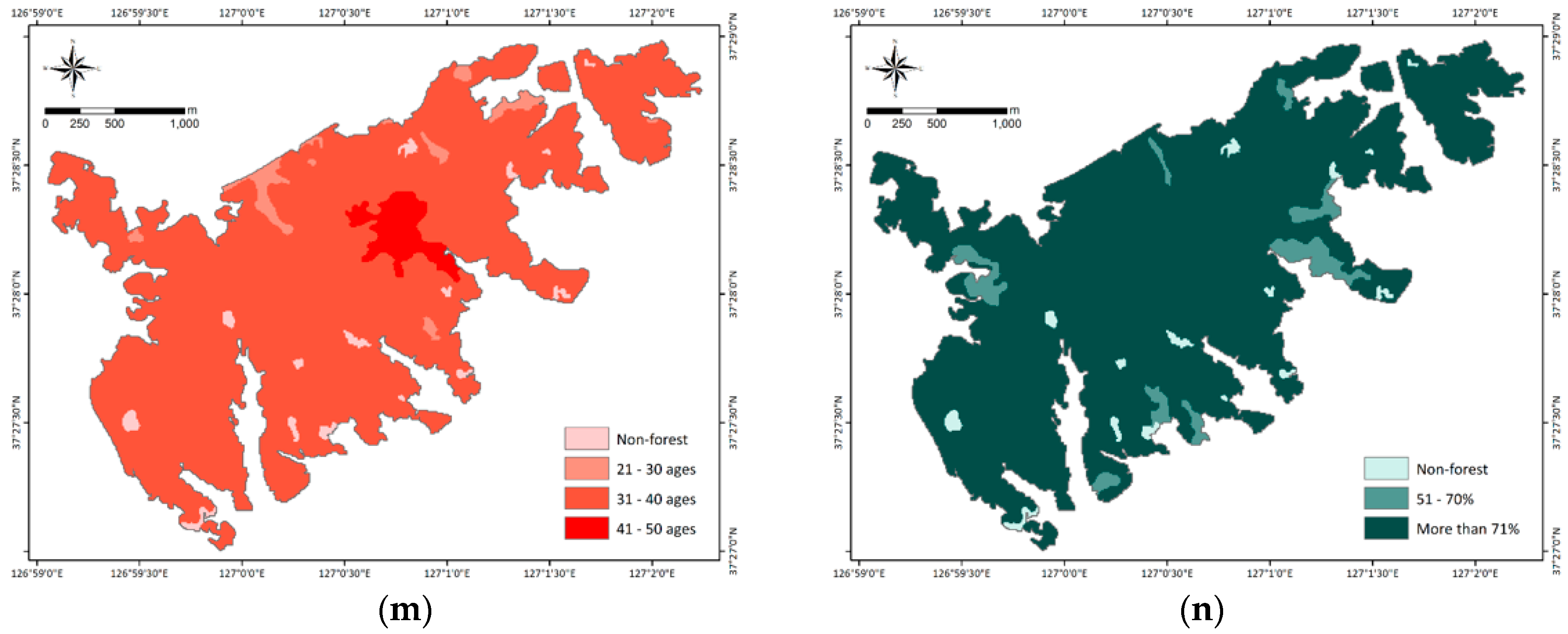
Vegetation prevents erosion on a slope by buffering the impact of rain falling on the slope, and vegetation roots increase the shear strength of the slope by increasing the shear strength of the soil. The forestry factors include timber type, timber diameter, timber age, and timber density. Here, timber type and timber age mean the species and average age of planted trees, respectively. In addition, timber diameter represents the size of the diameter at chest height. Timber density refers to the degree of closure of the crown canopy. These values were obtained from a 1:5000 scale forest map produced by the Korea Forest Research Institute.

3. Methodology

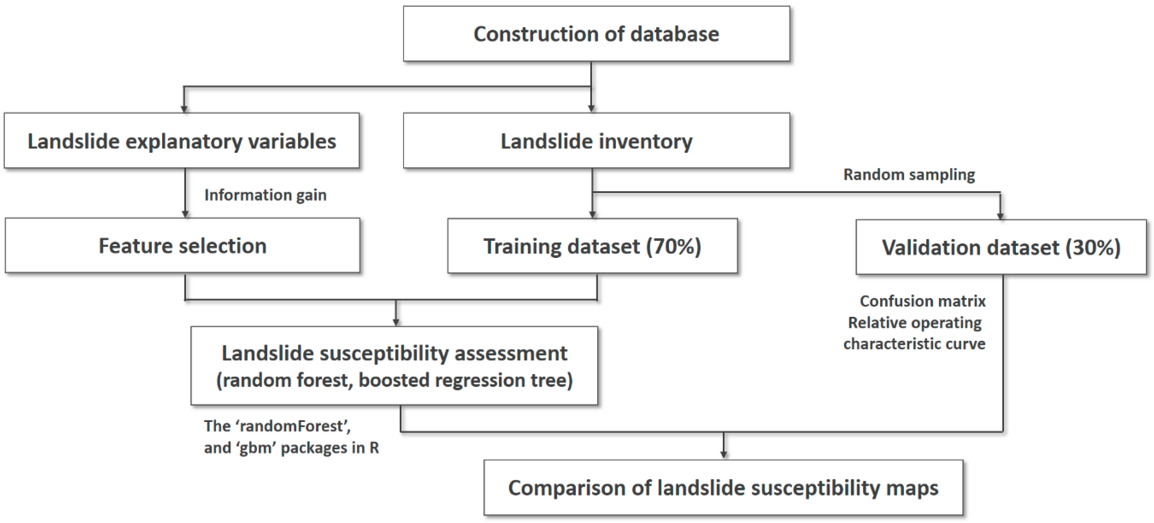
This study was performed using the following main steps: (1) collection and construction of database of landslides and landslide explanatory variables, (2) preparation of the training and test datasets through repeated random sampling, (3) feature selection using information gain (IG), (4) landslide susceptibility mapping using RF and BRT models, and (5) validation and comparison of performance among landslide susceptibility maps (LSMs) (Figure 2). The IG, RF, and BRT models were implemented in R (Foundation for Statistical Computing, Vienna, Austria) using the “FSelector,” “randomForest,” and “gbm” packages, respectively. These algorithms were performed employing a 10-fold cross-validation approach, to reduce the variability of the model results.

3.1. Landslide Dataset Preparation

In this study, correlations between landslide and landslide explanatory variables were analyzed using the FR (

Table A1. Correlations between landslide and landslide explanatory variables using the frequency ratio.

Factor	Class	No. of Pixels in Domains	No. of Landslide Pixels	Frequency Ratio	Normalized Frequency Ratio
Altitude (m)	[22.59, 66.57]	12,477	10	0.38	0.00
	[66.57, 95.90]	17,042	20	0.56	0.11
	[95.90, 126.35]	13,614	31	1.09	0.42
	[126.35, 159.05]	10,060	33	1.57	0.71
	[159.05, 196.27]	6766	17	1.20	0.49
	[196.27, 236.88]	4409	19	2.06	1.00
	[>236.88]	2637	10	1.81	0.85
Slope degree (°)	[0.00, 8.83]	4704	3	0.31	0.00
	[8.83, 13.98]	11,554	11	0.46	0.11
	[13.98, 18.15]	15,716	33	1.00	0.52
	[18.15, 22.07]	14,692	27	0.88	0.43
	[22.07, 26.24]	11,362	36	1.52	0.91
	[26.24, 31.39]	6708	23	1.64	1.00
	[>31.39]	2269	7	1.48	0.88
Slope aspect	Flat	69	0	0.00	0.00
	North	8483	12	0.68	0.50
	Northeast	7928	9	0.54	0.40
	East	9395	18	0.92	0.67
	Southeast	8837	20	1.08	0.80
	South	9522	26	1.31	0.96
	Southwest	8970	19	1.01	0.75
	West	6333	18	1.36	1.00
	Northwest	7468	18	1.15	0.85
Profile curvature	Concave	33,763	79	1.12	1.00
	Flat	247	0	0.00	0.00
	Convex	32,995	61	0.88	0.79
Plan curvature	Concave	31,592	82	1.24	1.00
	Flat	772	0	0.00	0.00
	Convex	34,641	58	0.80	0.65
Distance to streams (m)	[0.00, 167.16]	8947	3	0.61	0.28
	[167.16, 281.13]	12,553	16	1.46	0.81
	[281.13, 391.30]	13,430	41	0.77	0.38
	[391.30, 501.48]	12,372	20	1.28	0.69
	[504.48, 623.05]	9369	25	1.77	1.00
	[623.05, 763.61]	6205	23	1.39	0.76
	[>763.61]	4129	12	0.63	0.50
Topographic wetness index	[−7.19, −5.25]	8350	11	0.63	0.50
	[−5.25, −1.73]	3148	2	0.30	0.24
	[−1.73, 1.70]	13,316	24	0.86	0.69
	[1.70, 2.94]	21,415	56	1.25	1.00
	[2.94, 4.43]	14,843	38	1.23	0.98
	[4.43, 6.72]	4652	9	0.93	0.74
	[>6.72]	1281	0	0.00	0.00
Stream power index	[−13.82, −9.79]	487	0	0.00	0.00
	[−9.79, −8.40]	3850	2	0.25	0.17
	[−8.40, −4.54]	7251	11	0.73	0.48
	[−4.54, −0.35]	13,013	16	0.59	0.39
Stream power index	[−0.35, 0.88]	22,507	51	1.08	0.72
	[0.88, 2.60]	16,613	52	1.50	1.00
	[>2.60]	3284	8	1.17	0.78
Sediment transport index	[0.00, 4.35]	15,486	17	0.53	0.20
	[4.35, 10.88]	21,160	31	0.70	0.27
	[10.88, 16.87]	16,659	44	1.26	0.48
	[16.87, 24.49]	9054	29	1.53	0.58
	[24.49, 37.01]	3267	18	2.64	1.00
	[37.01, 58.23]	1065	0	0.00	0.00
	[>58.23]	314	1	1.52	0.58
Terrain roughness index	[0.00, 25.24]	6302	0	0.00	0.00
	[25.24, 33.92]	13,887	14	0.48	0.20
	[33.92, 42.20]	14,614	23	0.75	0.31
	[42.20, 51.30]	12,675	33	1.25	0.52
	[51.30, 61.64]	9415	27	1.37	0.57
	[61.64, 73.23]	6747	34	2.41	1.00
	[>73.23]	3365	9	1.28	0.53
Timber type	Non-forest	1027	0	0.00	0.00
	Pine	143	0	0.00	0.00
	Nut pine	2319	3	0.62	0.24
	Larch	1389	2	0.69	0.27
	Pitch pine	431	0	0.00	0.00
	Sawtooth oak	11,482	18	0.75	0.30
	Mongolian oak	1183	2	0.81	0.32
	Oriental oak	565	3	2.54	1.00
	Other oak	25,845	63	1.17	0.46
	Poplar	1419	6	2.02	0.80
	False acasia	15,809	30	0.91	0.36
	Other broadleaf forest	3707	12	1.55	0.61
	Mixed forest of soft and hardwood	1686	1	0.28	0.11
Timber diameter (cm)	Non-forest	1027	0	0.00	0.00
	[6, 16]	2124	3	0.68	0.66
	[16, 28]	63,854	137	1.03	1.00
Timber age (ages)	Non-forest	1027	0	0.00	0.00
	[21, 30]	1508	1	0.32	0.16
	[31, 40]	62,234	130	1.00	0.52
	[41, 50]	2236	9	1.93	1.00
Timber density (%)	Non-forest	1027	0	0.00	0.00
	[51, 70]	2994	5	0.80	0.78
	[>71]	62,984	135	1.03	1.00

). The FR is the ratio of the area where landslides occurred to the total study area. The FR was calculated by dividing the ratio of landslide occurrence, for the class or type of each factor, into an area ratio, for the class or type of each factor to the total area. The calculated FRs pertaining to each landslide explanatory variable were normalized from 0 to 1. The normalized FRs were extracted for the landslide and non-landslide dataset. Subsequently, these data were used for the training and validation datasets, to run the models and evaluate the prediction capabilities of the models, respectively.

3.2. Information Gain

The landslide explanatory variables have a crucial role in producing LSM. Some landslide explanatory variables might be associated with reductions in model performance, overfitting, model training time, and predictive capability [39]. Therefore, it is necessary to recognize and choose proper landslide explanatory variables.

Various methods such as IG [17], chi-square statistics [30], and Relief-F [29] have been proposed for feature selection in landslide modeling. In this study, the IG, proposed by Quinlan (1993) [40], was used to determine irrelevant and unimportant variables. The IG evaluates an attribute by determining the overall information gain in terms of the class. Consequently, the result can determine the ranking of importance, based on the normalized average merit contributed by each attribute [41,42].

The IG value of landslide explanatory variable $C_i$ belonging to class L (landslide and non-landslide) is calculated as [24,30]

$$IG\left(L, C_i\right)=IF\left(L\right)-IF(L|C_i),$$

(5)

where $IF\left(L\right)$ is the entropy value of L, and $IF(L|C_i)$ is the entropy of L after integrating the values of landslide explanatory variable $C_i$. These values are calculated using Equation (6) and Equation (7), respectively:

$$IF\left(L\right)=-{{\displaystyle \sum }}_{i}P\left(L_i\right){\log }_2\left(P\left(L_i\right)\right),$$

(6)

$$IF(L|C_i)=-{{\displaystyle \sum }}_{i}P\left(L_i\right){{\displaystyle \sum }}_{j}P\left(L_i|C_i)\right){\log }_2(P\left(L_i|C_i)\right),$$

(7)

where $P\left(L_i\right)$ is the prior probability of the class L, and $P\left(L_i|C_i\right)$ is the posterior probabilities of L given the values of explanatory variable $C_i$. An explanatory variable with a higher IG value has higher rank, meaning that it is more important to landslide models. By contrast, an explanatory variable with an IG value of zero must be removed from the dataset, because that factor does not make a contribution.

3.3. Landslide Susceptibility Analysis

3.3.1. Random Forest

RF, developed by Breiman (2001) [43], is a popular ensemble learning method that has been used widely for classification, regression, clustering, and interaction detection. A single decision tree is a weak classification, because of its high variance and bias. However, RF tends to produce robust models, because it can mitigate these problems by using ensemble trees [44].

RF generates thousands of random binary trees to form a forest. Each tree is grown based on a bootstrap sample, using a classification and regression trees (CART) procedure with a random subset of variables selected at each node [26,45]. For each tree grown on a bootstrap sample, the “out-of-bag” (OOB) error rate is calculated using observations left out of the bootstrap sample. The final decisions of class membership and model construction (output) are determined by the majority vote among all trees [46].

Two types of error rate—the mean decrease in accuracy and the mean decrease in the Gini coefficient—were calculated. These measures have been widely used to rank and select variables [26,47]. To run the RF model, the user should optimize two priori parameters, the number of trees in the forest (ntree) and the number of variables tested at each node (mtry), to minimize the OOB error and obtain good model performance [44,45].

3.3.2. Boosted Regression Tree Model

The BRT model is a combination of statistical and machine learning techniques. The BRT model fits different techniques and combines them to improve the performance of a single model [48,49]. Two different algorithms, namely boosting and regression, are used in the model, and the strengths of these algorithms are combined to improve model accuracy and decrease model variance [45,50]. Boosting is one of the most powerful learning methods for improving model accuracy, by iteratively fitting new trees to the residual errors (RE) of the existing tree assemblage [45,51]. In addition to boosting, the BRT model uses regression trees in the modeling process. Regression trees are categorized from the classification and regression tree approaches from the decision tree group of models [52].

In the model, among the various parameters, the number of trees is automatically set through internal cross-validation. In addition, the learning rate, the number of nodes in a single tree, and bag fraction were determined through a trial-and-error approach [53]. The complexity of the model and the contribution of each tree to the model are controlled by a shrinkage parameter and the learning rate, respectively. The bag fraction and shrinkage parameter determine the number of trees required to reach the optimal solution [54].

3.4. Model Performance Assessment and Comparison

3.4.1. Confusion Matrix

The confusion matrix includes true positive (TP), false positive (FP), true negative (TN), and false negative (FN) categories. Using these values, various statistical indices, such as accuracy, sensitivity, specificity, threat score, equitable threat score, Pierce’s skill score, odds ratio, and odds ratio skill score can be calculated [55]. The value calculated from the confusion matrix provides useful information on model performance and classification accuracy.

In this study, the sensitivity, specificity, overall accuracy, and kappa statistic were used to validate the performance of the LSMs. The percentages of landslide and non-landslide pixels classified correctly into those two categories enable the calculation of sensitivity and specificity, and the overall percentage classified correctly (in both categories together) indicates the accuracy of the LSMs [56]. In addition, the kappa statistic is used to evaluate the reliability of the landslide models. Its value ranges from −1 (non-reliable) to 1 (reliable) [57].

3.4.2. Receiver Operating Characteristic

The receiver operating characteristic (ROC) curve has been commonly used to validate the quality of a probabilistic model. The ROC curve is plotted by statistical index value pairs, with the false positive rate (sensitivity) on the x-axis and the “100−false negative rate” (100−specificity) on the y-axis. The ROC curve can be classified as a success rate curve or prediction rate curve, depending on the dataset used. The success rate curve, calculated using the training dataset, represents how well the LSMs fit the data. The prediction rate curve, calculated using the validation dataset, represents how well the model and landslide explanatory variables predict a landslide [11]. The ROC curve can be verified quantitatively when the area under the ROC curve (AUC) is calculated. AUC values range from 0.5 to 1.0. AUC values closer to 1 indicate a more accurate model.

4. Results

4.1. Selection of Landslide Explanatory Variables

The average information gain (AIG) value, and its standard deviation for each landslide explanatory variable, were calculated and ranked (

Table 2. Information gain values for the landslide explanatory variables used in this study.

No.	Landslide Explanatory Variable	Average Merit	Standard Deviation
1	Terrain roughness index	0.086	±0.010
2	Slope aspect	0.071	±0.012
3	Distance to streams	0.06	±0.010
4	Altitude	0.049	±0.008
5	Timber type	0.049	±0.008
6	Stream power index	0.041	±0.008
7	Slope degree	0.038	±0.008
8	Sediment transport index	0.037	±0.006
9	Topographic wetness index	0.033	±0.011
10	Plan curvature	0.025	±0.006
11	Profile curvature	0.013	±0.005
12	Timber age	0.012	±0.002
13	Timber density	0.008	±0.002
14	Timber diameter	0.005	±0.002

). All landslide explanatory variables used in this study contributed to the landslide models, because the AIG values of these variables were more than 0. According to the results, the TRI had the highest AIG value (0.086), which means that this factor made the greatest contribution to the landslide models in this study area. By contrast, timber diameter made the smallest contribution to the landslide models, as indicated by the lowest AIG value (0.005).

4.2. Training the Random Forest and Boosted Regression Tree Models

The training dataset was used to train the RF and BRT models for landslide susceptibility assessment. During the training process, the optimum values of the parameters for the models were applied to obtain high model predictive capability. The optimized values for the RF model were 300 for ntree and 2 for mtry. In the case of the BRT model, the optimized values for n.trees, interaction.depth, shrinkage, and n.minobsinnode were 500, 1, 0.01, and 10, respectively. Subsequently, the RF and BRT models were constructed using the optimized parameters, based on the training dataset. After their construction, the RF and BRT models were applied throughout the whole study area to produce LSMs.

4.3. Model Validation and Comparison

The performance of each model was analyzed using the training dataset. The RF model showed a higher sensitivity value (98.00%) than did the BRT model (79.57%). This result showed that the RF model classified more correctly than the BRT model in the landslide class. The specificity results also indicated that the RF model had higher specificity (100.00%) in the non-landslide class, indicating that the non-landslide pixels were more correctly classified. The specificity value of the BRT model was 76.70%. Because of the lower sensitivity and specificity values of the BRT model, the overall accuracy and kappa index values were lower, with values of 78.16% and 0.561, respectively. In the case of the RF model, the overall accuracy and kappa index were 98.98% and 0.980, respectively.

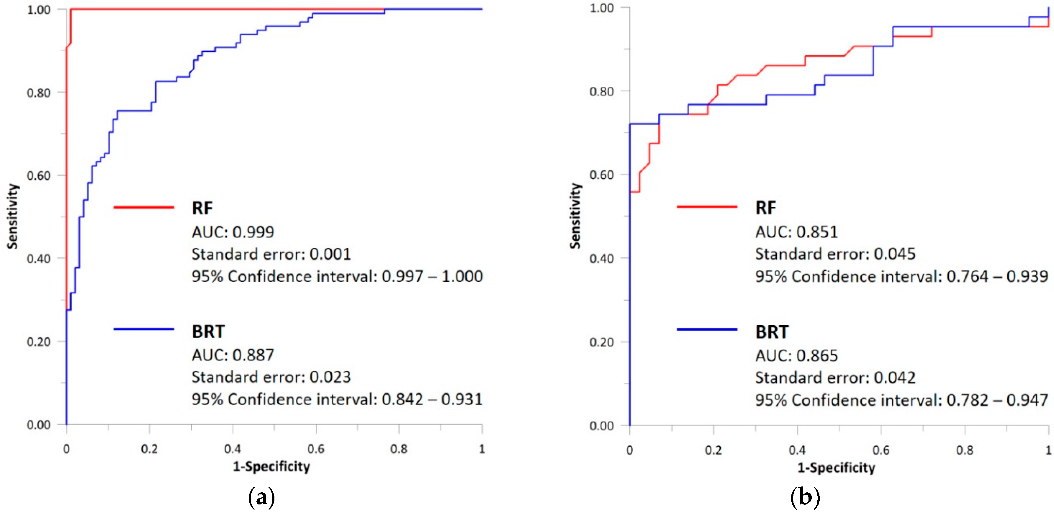
In addition, the success rate and the prediction rate were analyzed using the training dataset and the validation dataset, respectively (Figure 3). In the case of success rate, the RF and BRT models had values of 0.999 and 0.887, respectively. The prediction rate curve also showed that the RF model had a higher AUC (0.865) than the BRT model (0.851). Overall, the AUC values of all models were greater than 0.8. These results show that the LSMs constructed in this study have good accuracy in the spatial prediction of landslide susceptibility.

4.4. Generating Landslide Susceptibility Maps

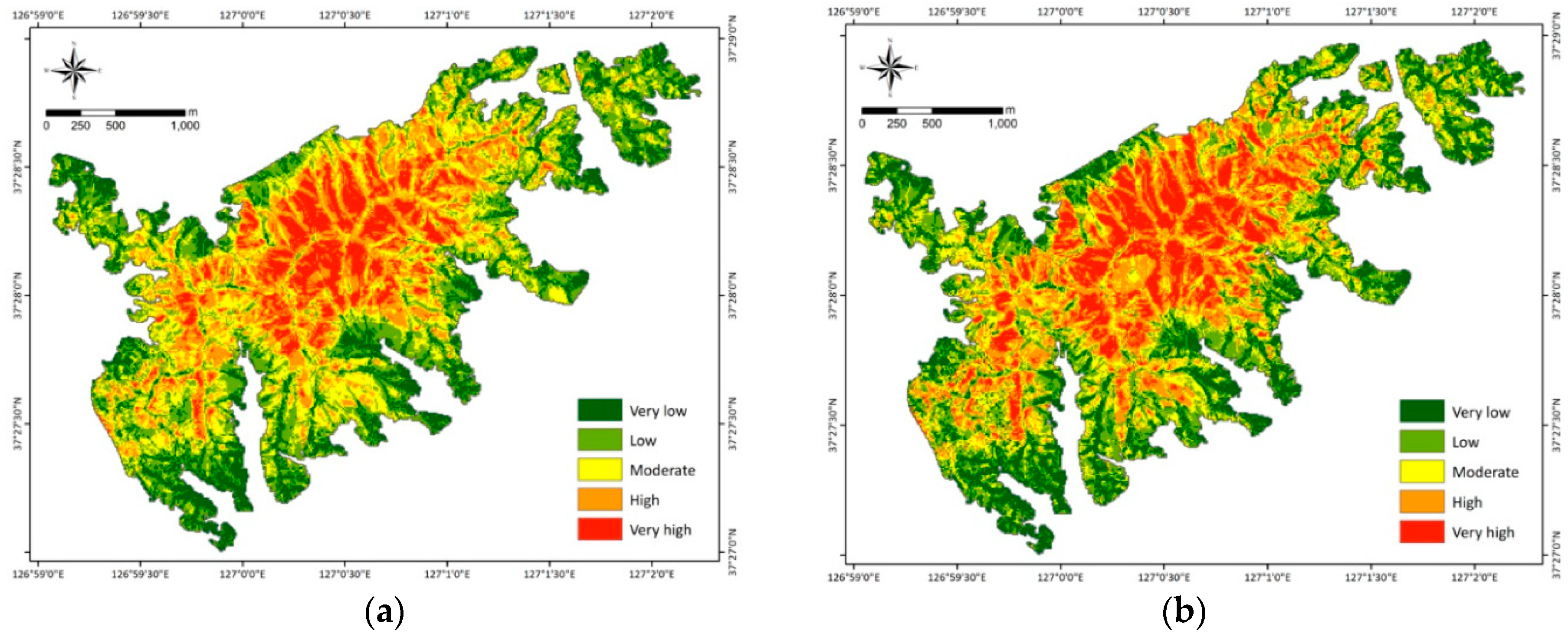
The RF and BRT models were used to develop LSMs in the study area. The LSMs were prepared by generating landslide susceptibility indices (LSIs) and reclassifying the class. The LSIs were calculated based on the trained RF and BRT models. Using the natural breaks method, the LSMs were reclassified into five susceptibility classes: very high, high, moderate, low, and very low (Figure 4). Overall, the distribution of LSI for each susceptibility class was similar between the LSM produced by RF (RF LSM) and that produced by BRT (BRT LSM). The “high” and “very high” susceptibility classes covered about 30% of the total area. The RF model had a value of 34.69%, and the BRT model had the lower value of 31.11%.

The LSMs produced from the two models were validated based on the landslide density (LD) of each susceptibility class on the LSMs. The LD is the ratio of the percentage of landslide pixels to the percentage of all pixels for each susceptibility class shown on the map [56]. LD was calculated by overlaying the five LSMs and the landslide inventory map. Generally, for the study area, the value of LD increased gradually, from very low to very high susceptibility (

Table 3. Landslide density on landslide susceptibility maps produced from the different models.

	Random Forest			Boosted Regression Tree
	Pixels of Class	Pixels of Landslide	Landslide Density	Pixels of Class	Pixels of Landslide	Landslide Density
Very low	13,034	2	0.073	10,671	3	0.135
Low	16,871	4	0.113	18,629	16	0.411
Moderate	13,854	16	0.553	16,860	35	0.994
High	12,917	36	1.334	12,930	41	1.518
Very high	10,329	82	3.799	7915	45	2.721
Total	67,005	140		67,005	140

). At the “very high” class, the RF and BRT models had LD values of 3.799 and 2.721, respectively. Overall, the models used in this study are suitable for LSM.

4.5. Discussion

The LSMs produced using the models were evaluated by statistical indices and ROC curves. The RF model had better sensitivity, specificity, overall accuracy, and kappa values. The AUC values of the LSMs used in this study were about 80%, indicating reasonable accuracy. The RF model had higher AUC values for the success rate and prediction rate curves than the BRT model. Thus, these models had very high predictive performance. Furthermore, the LSMs would be produced differently depending on the methods used and the landslide explanatory variables selected. The landslide explanatory variables may not make equal contributions, which can affect prediction ability. In this study, the landslide explanatory variables used made different contributions to the models.

Table 4. Relative importance of each landslide explanatory variable calculated in the random forest and boosted regression tree model.

	Random Forest		Boosted Regression Tree
	Importance	Rank	Importance	Rank
Terrain roughness index	1.000	1	1.000	1
Distance to streams	0.857	2	0.556	3
Altitude	0.766	3	0.277	5
Sediment transport index	0.654	4	0.562	2
Timber type	0.484	5	0.158	7
Slope degree	0.469	6	0.000	-
Stream power index	0.449	7	0.084	9
Topographic wetness index	0.440	8	0.378	4
Slope aspect	0.408	9	0.242	6
Plan curvature	0.214	10	0.099	8
Profile curvature	0.118	11	0.016	10
Timber diameter	0.026	12	0.000	-
Timber age	0.009	13	0.000	-
Timber density	0.000	14	0.000	-

illustrates the importance of each explanatory variable, calculated and normalized in the RF and BRT models. In general, TRI had the highest importance to the models, whereas timber diameter, timber age, and timber density had lower predictive capability.

From the results, ensemble classification, such as that done by the model used in this study, can improve the performance of single (weak) classifiers and the prediction accuracy of LSM [56]. However, the models had overfitting problems, as indicated by the AUC values calculated using the training and validation datasets. The AUC values of the success rate curve were very high, almost reaching a value of 1, but the AUC values of the prediction rate curve were lower. Especially in the case of the RF model, the AUC value of the prediction rate was decreased by about 20%. This result showed that the RF model was trained excessively by the training data. This can be associated with poor generalization from training data and increased error for real data. Overfitting is a common problem affecting researchers performing machine learning and data mining. There can be many reasons for overfitting. However, in this study, the landslide explanatory variables used still included noise, despite the feature selection process. In addition, because the landslide area is very small compared to the non-landslide area, the model could not learn and predict the non-landslide area.

5. Conclusions

This study compared and analyzed landslide susceptibility at Woomyeon Mountain using different models. For this purpose, landslide-related spatial data consisting of a landslide inventory, and landslide explanatory variables were collected and prepared. The landslide inventory map was built using aerial photographs. The 14 landslide explanatory variables were constructed from spatial data collected by government organizations. These factors included altitude, slope degree, slope aspect, profile curvature, plan curvature, distance to streams, TWI, SPI, STI, TRI, timber type, timber diameter, timber age, and timber density.

The contribution of each landslide explanatory variable was evaluated using the average IG value with a 10-fold cross-validation approach. All of the landslide explanatory variables contributed to the models, because the IG values of all factors were greater than zero. Therefore, the landslide susceptibility analysis and mapping were performed with all landslide explanatory variables using the RF and BRT models. The RF and BRT models were implemented in R. A popular open-source software, R is helpful for statistical computing and data visualization [58]. The models were constructed using optimized parameters, and LSI was predicted over the study area.

The LSMs produced in this study may prove useful for decision makers, planners, and engineers in disaster planning to minimize economic losses and casualties. In a future study, the accuracy of the LSMs of this study could be enhanced by selecting more optimal landslide explanatory variables and solving the problem of overfitting.

References

- Das, I.; Stein, A.; Kerle, N.; Dadhwal, V.K. Landslide susceptibility mapping along road corridors in the Indian Himalayas using Bayesian logistic regression models. Geomorphology 2012, 179, 116–125. [Google Scholar] [CrossRef]
- Jakob, M.; Lambert, S. Climate change effects on landslides along the southwest coast of British Columbia. Geomorphology 2009, 107, 275–284. [Google Scholar] [CrossRef]
- Vasu, N.N.; Lee, S.R. A hybrid feature selection algorithm integrating an extreme learning machine for landslide susceptibility modeling of Mt Woomyeon, South Korea. Geomorphology 2016, 263, 50–70. [Google Scholar] [CrossRef]
- Park, S.; Choi, C.; Kim, B.; Kim, J. Landslide susceptibility mapping using frequency ratio, analytic hierarchy process, logistic regression, and artificial neural network methods at the Inje area, Korea. Environ. Earth Sci. 2013, 68, 1443–1464. [Google Scholar] [CrossRef]
- Schuster, R.L. Socioeconomic Significance of Landslides: Investigation and Mitigation; National Academy Press Transportation Research Board Special Report; National Academy Press: Washington, DC, USA, 1996; Volume 247, pp. 12–35. [Google Scholar]
- Guzzetti, F.; Reichenbach, P.; Ardizzone, F.; Cardinali, M.; Galli, M. Estimating the quality of landslide susceptibility models. Geomorphology 2006, 81, 166–184. [Google Scholar] [CrossRef]
- Mohammady, M.; Pourghasemi, H.R.; Pradhan, B. Landslide susceptibility mapping at Golestan Province, Iran: A comparison between frequency ratio, Dempster–Shafer, and weights-of-evidence models. J. Asian Earth Sci. 2012, 61, 221–236. [Google Scholar] [CrossRef]
- Akgun, A.; Dag, S.; Bulut, F. Landslide susceptibility mapping for a landslide-prone area (Findikli, NE of Turkey) by likelihood-frequency ratio and weighted linear combination models. Environ. Geol. 2008, 54, 1127–1143. [Google Scholar] [CrossRef]
- Yilmaz, I. Landslide susceptibility mapping using frequency ratio, logistic regression, artificial neural networks and their comparison: A case study from Kat landslides (Tokat—Turkey). Comput. Geosci. 2009, 35, 1125–1138. [Google Scholar] [CrossRef]
- Kanungo, D.P.; Sarkar, S.; Sharma, S. Combining neural network with fuzzy, certainty factor and likelihood ratio concepts for spatial prediction of landslides. Nat. Hazards 2011, 59, 1491–1512. [Google Scholar] [CrossRef]
- Bui, D.T.; Lofman, O.; Revhaug, I.; Dick, O. Landslide susceptibility analysis in the Hoa Binh Province of Vietnam using statistical index and logistic regression. Nat. Hazards 2011, 59, 1413–1444. [Google Scholar] [CrossRef]
- Zhang, G.; Cai, Y.; Zheng, Z.; Zhen, J.; Liu, Y.; Huang, K. Integration of the statistical index method and the analytic hierarchy process technique for the assessment of landslide susceptibility in Huizhou, China. Catena 2016, 142, 233–244. [Google Scholar] [CrossRef]
- Ozdemir, A.; Altural, T. A comparative study of frequency ratio, weights of evidence and logistic regression methods for landslide susceptibility mapping: Sultan Mountains, SW Turkey. J. Asian Earth Sci. 2013, 64, 180–197. [Google Scholar] [CrossRef]
- Xu, C.; Xu, X.; Lee, Y.H.; Tan, X.; Yu, G.; Dai, F. The 2010 Yushu earthquake triggered landslide hazard mapping using GIS and weight of evidence modeling. Environ. Earth Sci. 2012, 66, 1603–1616. [Google Scholar] [CrossRef]
- Pourghasemi, H.R.; Moradi, H.R.; Aghda, S.F. Landslide susceptibility mapping by binary logistic regression, analytical hierarchy process, and statistical index models and assessment of their performances. Nat. Hazards 2013, 69, 749–779. [Google Scholar] [CrossRef]
- Yalcin, A.; Reis, S.; Aydinoglu, A.C.; Yomralioglu, T. A GIS-based comparative study of frequency ratio, analytical hierarchy process, bivariate statistics and logistics regression methods for landslide susceptibility mapping in Trabzon, NE Turkey. Catena 2011, 85, 274–287. [Google Scholar] [CrossRef]
- Chen, W.; Shirzadi, A.; Shahabi, H.; Ahmad, B.B.; Zhang, S.; Hong, H.; Zhang, N. A novel hybrid artificial intelligence approach based on the rotation forest ensemble and naïve Bayes tree classifiers for a landslide susceptibility assessment in Langao County, China. Geomat. Nat. Hazards 2017, 8, 1955–1977. [Google Scholar] [CrossRef] [Green Version]
- Jordan, M.; Mitchell, T. Machine learning: Trend, perspectives, and prospects. Science 2015, 349, 255–260. [Google Scholar] [CrossRef] [PubMed]
- Gomez, H.; Kavzoglu, T. Assessment of shallow landslide susceptibility using artificial neural networks in Jabonosa River Basin, Venezuela. Eng. Geol. 2005, 78, 11–27. [Google Scholar] [CrossRef]
- Nefeslioglu, H.A.; Gokceoglu, C.; Sonmez, H. An assessment on the use of logistic regression and artificial neural networks with different sampling strategies for the preparation of landslide susceptibility maps. Eng. Geol. 2008, 97, 171–191. [Google Scholar] [CrossRef]
- Shahabi, H.; Hashim, M.; Ahmad, B.B. Remote sensing and GIS-based landslide susceptibility mapping using frequency ratio, logistic regression, and fuzzy logic methods at the central Zab basin, Iran. Environ. Earth Sci. 2015, 73, 8647–8668. [Google Scholar] [CrossRef]
- Zhu, A.X.; Wang, R.; Qiao, J.; Qin, C.Z.; Chen, Y.; Liu, J.; Zhu, T. An expert knowledge-based approach to landslide susceptibility mapping using GIS and fuzzy logic. Geomorphology 2014, 214, 128–138. [Google Scholar] [CrossRef]
- Vahidnia, M.H.; Alesheikh, A.A.; Alimohammadi, A.; Hosseinali, F. A GIS-based neuro-fuzzy procedure for integrating knowledge and data in landslide susceptibility mapping. Comput. Geosci. 2010, 36, 1101–1114. [Google Scholar] [CrossRef]
- Bui, D.T.; Ho, T.C.; Pradhan, B.; Pham, B.T.; Nhu, V.H.; Revhaug, I. GIS-based modeling of rainfall-induced landslides using data mining-based functional trees classifier with AdaBoost, Bagging, and MultiBoost ensemble frameworks. Environ. Earth Sci. 2016, 75, 1101. [Google Scholar]
- Kavzoglu, T.; Sahin, E.K.; Colkesen, I. An assessment of multivariate and bivariate approaches in landslide susceptibility mapping: A case study of Duzkoy district. Nat. Hazards 2015, 76, 471–496. [Google Scholar] [CrossRef]
- Pourghasemi, H.R.; Kerle, N. Random forests and evidential belief function-based landslide susceptibility assessment in Western Mazandaran Province, Iran. Environ. Earth Sci. 2016, 75, 1–17. [Google Scholar] [CrossRef]
- Youssef, A.M.; Pourghasemi, H.R.; Pourtaghi, Z.S.; Al-Katheeri, M.M. Landslide susceptibility mapping using random forest, boosted regression tree, classification and regression tree, and general linear models and comparison of their performance at Wadi Tayyah Basin, Asir Region, Saudi Arabia. Landslides 2015, 13, 1–18. [Google Scholar]
- Tsangaratos, P.; Ilia, I. Comparison of a logistic regression and Naïve Bayes classifier in landslide susceptibility assessments: The influence of models complexity and training dataset size. Catena 2016, 145, 164–179. [Google Scholar] [CrossRef]
- Hong, H.; Liu, J.; Bui, D.T.; Pradhan, B.; Acharya, T.D.; Pham, B.T.; Ahmad, B.B. Landslide susceptibility mapping using J48 Decision Tree with AdaBoost, Bagging and Rotation Forest ensembles in the Guangchang area (China). Catena 2018, 163, 399–413. [Google Scholar] [CrossRef]
- Pham, B.T.; Bui, D.T.; Dholakia, M.B.; Prakash, I.; Pham, H.V.; Mehmood, K.; Le, H.Q. A novel ensemble classifier of rotation forest and Naïve Bayer for landslide susceptibility assessment at the Luc Yen district, Yen Bai Province (Viet Nam) using GIS. Geomat. Nat. Hazards Risk 2017, 8, 649–671. [Google Scholar] [CrossRef]
- Korean Geotechnical Society (KGS). The Study on Investigation of Cause and Development of Restoration Policy about Landslide in Wumyon Area; Korean Geotechnical Society: Seoul, Korea, 2011. (In Korean) [Google Scholar]
- Cao, C.; Xu, P.; Wang, Y.; Chen, J.; Zheng, L.; Niu, C. Flash flood hazard susceptibility mapping using frequency ratio and statistical index methods in coalmine subsidence areas. Sustainability 2016, 8, 948. [Google Scholar] [CrossRef]
- Kalantar, B.; Pradhan, B.; Naghibi, S.A.; Motevalli, A.; Mansor, S. Assessment of the effects of training data selection on the landslide susceptibility mapping: A comparison between support vector machine (SVM), logistic regression (LR) and artificial neural networks (ANN). Geomat. Nat. Hazards Risk 2018, 9, 49–69. [Google Scholar] [CrossRef]
- Beven, K.J.; Kirkby, M.J. A physically based, variable contributing area model of basin hydrology/Un modèle à base physique de zone d’appel variable de l’hydrologie du bassin versant. Hydrol. Sci. J. 1979, 24, 43–69. [Google Scholar] [CrossRef]
- Poudyal, C.P.; Chang, C.; Oh, H.J.; Lee, S. Landslide susceptibility maps comparing frequency ratio and artificial neural networks: A case study from the Nepal Himalaya. Environ. Earth Sci. 2010, 61, 1049–1064. [Google Scholar] [CrossRef]
- Moore, I.D.; Grayson, R.B.; Ladson, A.R. Digital terrain modelling: A review of hydrological, geomorphological, and biological applications. Hydrol. Process. 1991, 5, 3–30. [Google Scholar] [CrossRef]
- Moore, I.D.; Burch, G.J. Sediment transport capacity of sheet and rill flow: Application of unit stream power theory. Water Resour. Res. 1986, 22, 1350–1360. [Google Scholar] [CrossRef]
- Althuwaynee, O.F.; Pradhan, B.; Park, H.J.; Lee, J.H. A novel ensemble bivariate statistical evidential belief function with knowledge-based analytical hierarchy process and multivariate statistical logistic regression for landslide susceptibility mapping. Catena 2014, 114, 21–36. [Google Scholar] [CrossRef]
- Liu, H.; Motoda, H. Ensemble-based variable selection using independent probes. In Computational Methods of Feature Selection; Chapman and Hall/CRC: London, UK, 2007; pp. 147–162. [Google Scholar]
- Quinlan, J.T. C4.5: Programs for Machine Learning; Morgan Kaufmann Publishers: San Francisco, CA, USA, 1993. [Google Scholar]
- Oommen, T.; Cobin, P.F.; Gierke, J.S.; Sajinkumar, K.S. Significance of variable selection and scaling issues for probabilistic modeling of rainfall-induced landslide susceptibility. Spat. Inf. Res. 2018, 26, 21–31. [Google Scholar] [CrossRef]
- Witten, I.G.; Frank, E. Data Mining: Practical Machine Learning Tools and Techniques, 2nd ed.; Morgan Kaufmann Publishers: San Francisco, CA, USA, 2005. [Google Scholar]
- Breiman, L. Random forests. Mach. Learn. 2001, 45, 5–32. [Google Scholar] [CrossRef]
- Taalab, K.; Cheng, T.; Zhang, Y. Mapping landslide susceptibility and types using Random Forest. Big Earth Data 2018, 2, 1–20. [Google Scholar] [CrossRef]
- Rahmati, O.; Naghibi, S.A.; Shahabi, H.; Bui, D.T.; Pradhan, B.; Azareh, A.; Melesse, A.M. Groundwater spring potential modelling: Comprising the capability and robustness of three different modeling approaches. J. Hydrol. 2018, 565, 248–261. [Google Scholar] [CrossRef]
- Micheletti, N.; Foresti, L.; Robert, S.; Leuenberger, M.; Pedrazzini, A.; Jaboyedoff, M.; Kanevski, M. Machine learning feature selection methods for landslide susceptibility mapping. Math. Geosci. 2014, 46, 33–57. [Google Scholar] [CrossRef]
- Calle, M.L.; Urrea, V. Letter to the editor: Stability of random forest importance measures. Brief Bioinform. 2010, 12, 86–89. [Google Scholar] [CrossRef] [PubMed]
- Schapire, R.E. The boosting approach to machine learning: An overview. In Nonlinear Estimation and Classification; Springer: New York, NY, USA, 2003; pp. 149–171. [Google Scholar]
- Elith, J.; Leathwick, J.R.; Hastie, T. A working guide to boosted regression trees. J. Anim. Ecol. 2008, 77, 802–813. [Google Scholar] [CrossRef] [PubMed] [Green Version]
- Aertsen, W.; Kint, V.; Van Orshoven, J.; Özkan, K.; Muys, B. Comparison and ranking of different modelling techniques for prediction of site index in Mediterranean mountain forests. Ecol. Model. 2010, 221, 1119–1130. [Google Scholar] [CrossRef]
- Cao, D.S.; Xu, Q.S.; Liang, Y.Z.; Zhang, L.X.; Li, H.D. The boosting: A new idea of building models. Chemom. Intell. Lab. 2010, 100, 1–11. [Google Scholar] [CrossRef]
- Naghibi, S.A.; Pourghasemi, H.R.; Abbaspour, K. A comparison between ten advanced and soft computing models for groundwater qanat potential assessment in Iran using R and GIS. Theor. Appl. Climatol. 2018, 131, 967–984. [Google Scholar] [CrossRef]
- França, S.; Cabral, H.N. Predicting fish species richness in estuaries: Which modelling technique to use? Environ. Model. Softw. 2015, 66, 17–26. [Google Scholar] [CrossRef]
- Al-Abadi, A.M. A novel geographical information system-based Ant Miner algorithm model for delineating groundwater flowing artesian well boundary: A case study from Iraqi southern and western deserts. Environ. Earth Sci. 2017, 76, 534. [Google Scholar] [CrossRef]
- Frattini, P.; Crosta, G.; Carrara, A. Techniques for evaluating the performance of landslide susceptibility models. Eng. Geol. 2010, 111, 62–72. [Google Scholar] [CrossRef]
- Pham, B.T.; Bui, D.T.; Dholakia, M.B.; Prakash, I.; Pham, H.V. A comparative study of least square support vector machines and multiclass alternating decision trees for spatial prediction of rainfall-induced landslides in a tropical cyclones area. Geotech. Geol. Eng. 2016, 34, 1807–1824. [Google Scholar] [CrossRef]
- Bennett, N.D.; Croke, B.F.; Guariso, G.; Guillaume, J.H.; Hamilton, S.H.; Jakeman, A.J.; Pierce, S.A. Characterising performance of environmental models. Environ. Model. Softw. 2014, 40, 1–20. [Google Scholar] [CrossRef]
- Zhou, J.; Li, X.; Mitri, H.S. Classification of rockburst in underground projects: Comparison of ten supervised learning methods. J. Comput. Civ. Eng. 2016, 30, 04016003. [Google Scholar] [CrossRef]
Figure 1.
Location of study area (a) and landslide inventory map with hill shading (b).
Figure 2.
Flow chart of the overall methodology.
Figure 3.
Analysis of the receiver operating characteristic (ROC) curve for the two landslide susceptibility maps: (a) success rate curve using the training dataset and (b) prediction rate curve using the validation dataset.
Figure 4.
Landslide susceptibility maps produced by random forest (RF) (a) and boosted regression tree (BRT) (b) models.