Testing Procedure of Unmanned Aerial Vehicles (UAVs) Trajectory in Automatic Missions


AGH University of Science and Technology, Faculty of Mining Surveying and Environmental Engineering, 30-059 Cracow, Poland
Appl. Sci. 2019, 9(17), 3488; https://0-doi-org.brum.beds.ac.uk/10.3390/app9173488
Submission received: 31 July 2019
/
Revised: 20 August 2019
/
Accepted: 20 August 2019
/
Published: 23 August 2019
(This article belongs to the Special Issue Unmanned Aerial Vehicles (UAVs))
Abstract
:This paper describes an experimental test campaign while using an Unmanned Aerial Vehicle (UAV) and measuring the obtained UAV positions during different flight tasks and in different operative conditions. A new test procedure has been presented and tested for different devices in various weather conditions. This paper describes and analyses the measurements of the flight trajectory of the UAV that was performed with the use of a robotic total station (RTS), as compared to the design data and the data recorded in the internal memory of the UAV. Five different test tasks have been conducted. The obtained results have allowed for the assessment of the correctness of task performance as compared to the design and to determine the flying accuracy of the entire UAV set. The proposed set of tasks can be successfully utilised to control the correctness of operation of various types of UAVs and it may be implemented as a universal test to verify the algorithms optimising take-offs and landings, test flights of the objects, as well as flight planning in various terrain and weather conditions, which will increase the safety of the flights while using UAVs.
1. Introduction
The use of unmanned aerial vehicles (UAV) in a wide variety of domains of economy allows for accelerating the performance of various tasks. UAVs increase both the level of security of property and people as well as allowing initiating completely new uses. This equipment has recently become very popular for logistics and surveillance applications [1]. Thanks to a possibility of embedding several transmitters, sensors, and photographing equipment, UAVs can be used in a wide range of applications. Successful cases have been reported in, e.g., aerial reconnaissance [2], aerial forest fire detection [3], target observation [4], traffic monitoring and management [5], smart city [6], online commerce [7], geographic monitoring [8], scientific data collection [9], meteorological sampling [10], photogrammetry and three-dimensional mapping [2,9,11,12,13,14], UAVs networks [15], humanitarian relief [16], and disaster assessment and response [17,18,19]. More examples of the fast expanding potential of UAVs are presented in Rao et al. and Wyngaard et al. [20,21].
In June 2018, the European Parliament voted to adopt a new regulation that is the first one to regulate the UAV market [22]. Its development is currently being inhibited by uncoordinated national regulations, which hinders the implementation of the European Union (EU) idea of the Urban Space (U-Space)—a special airspace for automatic and autonomous flights out of sight in cities. The unification of the regulations will open the door for the further development of the drone market and popularisation of UAVs. On the other hand, UAVs are getting increasingly distanced from classical aviation and they are becoming flying robots. The growing requirements that are related to ensuring high safety levels of flight operations, as well as the legal regulations will force the certification of UAVs. According to the author, one of the stages of certification of this type of equipment should involve tests that allow for defining the characteristics that determine the correctness of the UAV task implementation. The missions that are performed by UAVs can be performed in automatic mode with the device implementing a previously planned mission, or autonomous at various levels of autonomy [23]. The navigation starts with the analysis of the environment using sensors (laser, stereo-vision, time-of-flight analysis), the modelling of the environment, the positioning using data integration techniques from navigation sensors (GNSS—Global Navigation Satellite System, IMU—Inertial Measurement Unit, gyroscopes), and the movement control using the ability to plan the path. The most advanced solutions in autonomous navigation are the algorithms that include the creation of a map into a navigation task, the so-called SLAM (Simultaneous Localisation and Mapping) [24,25]. There are also works being carried out that focus on the preparation of the ICT (Information and Communications Technologies) systems that support the UAV missions, as exemplified by the implementation of the contact system of the air traffic service units with the UAV operators, performed by the company DronRadar [26]. The UAV automatic take-off and landing systems are also being created [27]. According to the planned regulations, the drones that are to fly in the EU sky in the future will have to be equipped with certain elements, such as an altimeter, a device defining the position, geographical zone, and the maximum allowable operating distance, as well as collision avoidance and automatic landing systems. The European Parliament argues that it is about ensuring safety [22]. In addition, the studies into optimisation of the UAV flight trajectories are currently being conducted in numerous research centres. The performed research is aimed at the optimisation of image coverage of the areas subject to photogrammetric measurements [11,28,29], at improving the inspection of objects [30,31,32,33] as well as the trajectory of changes in flight directions [34,35].
While taking into account the rapid development of UAVs, it should be noted that the research has been carried out in different directions. The studies of mathematical models of a vehicle movement trajectory, structural models of machines, testing their reliability by developing appropriate procedures and methods of the research are among the most important ones [30,34,35]. The results of such analyses include the parameters that can be used to optimise the performance and durability, to determine the reliability, safety, and effective operation of the systems. In the case of unmanned aerial vehicles, it is essential to identify the possibilities of their control.
The studies that were conducted in this research paper have aimed to develop a new set of tests for measuring the position of UAVs in space. In the set of tests that were proposed by the author, the navigation using the GNSS system, magnetometer, IMU assisted with baro-sensors, has been subject to the studies. It should be noted that these elements are the basic components that are used by on-board computers when controlling UAVs. The performed tests will allow for the use of UAVs in specific missions that require flights with small horizontal and vertical separations [31,36], at precisely determined altitudes [12,25,33] and in areas with a complex terrain morphology [37,38]. In addition, the procedures that were proposed in this research paper will allow verifying the algorithms that optimise the test flights of the objects in reality. The targets of these explore-and-exploit approaches are many fold, such as maximizing the coverage of a target object or minimizing the acquisition time or energy consumption [36]. They will also allow for the introduction of additional parameters in the models, resulting from the measurement of the actual flight trajectory. In [39], the authors propose a method that can be used to model and analyse the energy consumption of a specific drone as a function of its speed and operating conditions.
2. Materials and Methods-Test Tasks for UAVs and Field Works
The studies that are discussed in this paper are a significant extension and continuation of the research presented in [40,41]. The first paper discusses the results of the research that aimed at determining the accuracy of stabilisation of an unmanned aerial system. The tests have been performed for the DJI S900 device with the A2 on-board computer during basic aviation operations. All of the manoeuvres have been performed in the remote control (RC) mode. The position of the UAV has been stabilised by its on-board systems. The first test has been aimed at determining the hovering accuracy by the UAV. It has been divided into two parts that differed in the duration of the measurement (5 min. and 10 min.). The second stage has been aimed at determining the accuracy of the UAV making horizontal and vertical displacements by the predetermined value. The second paper [41] discusses the tests that were conducted in an automatic mode where the basic measurements that are contained in the standards for industrial robots have been performed. The commonly used definition of the UAV for flying devices utilised for the purposes other than recreational or sport ones, says that it is an aircraft that does not require a crew to be present on board and it is unable to take passengers, it is controlled remotely or performs automatic flights. The definition of an industrial robot is as follows: a manipulative industrial robot is an automatically controlled, reprogrammable, multi-purpose manipulation machine with multiple degrees of freedom, having manipulative or locomotive properties, stationary or mobile, for important industrial applications [42]. When considering the above definitions, UAVs can be classified as mobile industrial robots. The paper [41] has analysed the selected tests that are presented in the ISO standard [43] with view to their implementation in the measurements of the UAV positioning accuracy. The works that are discussed there have aimed at verifying the suitability of these standards to examine the UAV positioning accuracy and they have been carried out for one on-board computer. An extended set of these tests has also been presented in this paper as task 2 cf. Section 2.
The first UAV trajectory tracking measurements were carried out by Eisenbeiss [44]. An automatic flight trajectory tracker, while using a robotic total station (RTS), has been the first of its kind performed on a UAV system. RTS is a surveying instrument that allows for automatic target search, recognition, and tracking. A test field for UAVs has also been established at the campus of Hönggerberg at ETH Zurich. This test field has enabled assess to the flight performance of UAVs. The tests that have been performed in this study have only included the analysis of the accuracy of a photogrammetric mission performed on a small-sized test basis. Basic flight trajectory analyses have been carried out. Similar but more complex tests were described in this paper as task 4 cf. Section 2. In Bláha et al. [45], the authors have focused on the analysis of the potential of the positioning accuracy of the UAV system Falcon 8. Consequently, the parameters of the positions, which are also co-determined in the process of direct geo-referencing, have not been considered there. This paper has focused on the comparison of the results from GNSS to direct geo-referencing. In addition, in this paper, the authors have demonstrated that the positioning results using direct geo-referencing have been able to provide information on the accuracy of which a drone can be positioned with. It is lower than what is available while using the prism tracking RTS. Paper [46] provides an alternative method for aerial vehicle localization and control utilising standard construction equipment suitable for onsite fabrication. The three-dimensional (3D) distances between reference and effective flight path have been analysed in order to evaluate the control quality for the RTS guided UAV. In these tests, the studies were conducted in a very little space, in a cube of a size of not more than 15 m. As demonstrated in works [47,48], the use of a RTS allows for a significantly more accurate means of empirical modelling of the sensor measurement variance of localization systems. From this, an effective extended Kalman filter system was designed and shown to function well in its intended environment in comparison to the raw UWB (Ultra Wide Band) positioning algorithm. The RTS has been previously demonstrated as both an effective source of reference data for the assessment of accuracy of state estimation systems, and also as a means of characterizing the sensor variance. The suitability of the RTS is confirmed in [49], where kinematic positioning was applied to a UAV in a field trial to improve a priori image coordinates and evaluate the method for direct geo-referencing. The premise of this research was to replace GNSS navigation quality (1–10 m) coordinates that were used as a priori positions for photogrammetric processing with higher-precision image positions derived from a RTS. This required a detailed investigation of kinematic positioning with a RTS. Moreover, testing the performance characteristics of Micro-Electro-Mechanical Systems (MEMS) or low cost navigation sensors for various UAV applications is important research [50]. This work focuses on studying the performance characteristics under different manoeuvres while using inertial measurements that were integrated with single point positioning, Real-Time-Kinematic (RTK), and additional navigational aiding sensors. Furthermore, the performance of the inertial sensors is tested during GNSS signal outage. RTK or post-processed kinematic (PPK) methods are also used for the georeferencing of measurement materials (photos, LIDAR scans), but these solutions are not commonly used for UAV navigation [29,51,52]. Papers [53,54,55] also include the information on the application of the systems utilising camera systems that create systems allowing trajectory tracking and defining based on the image. The UAV tracking with the use of high speed cameras could be implemented in small areas, while for larger areas, due to the limitation of the field of view of the camera, a new construction of the measuring system for the automatic target tracking would be necessary. It should be emphasised that such systems have much lower accuracy of determining the coordinates as well as a smaller range. Therefore, the proposed measurement methodology may prove to be very helpful in assessing the accuracy of their operation.
The UAV trajectory tracking studies that have been conducted so far have mainly focused on the use of new measurement methods. However, to the best of author knowledge, none of these works take into account the positioning accuracy of on-board computer and control systems in the realization of UAV missions. The tests that were carried out by Eisenbaiss [44] concerned only one type of UAV mission, and the systems that are described in [53,54,55] did not give sufficient accuracy in determining the coordinates. On the other hand, UWB systems had a limited range of operation [47]. In contrast to the studies that are described above in this article, an innovative set of tests has been proposed, which allows for assessing the accuracy of the task performance by UAV in space. Taking into account the state-of-the-art, the RTS was used during the research for reference measurements determining the current position of the UAV. The RTS was used with geodetic prisms (360° mini prism). It is an accurate, widely available and the most reliable method of tracking trajectories of objects in motion. The suitability and versatility of the proposed tests were verified by conducting appropriate field works for two different devices in various weather conditions.
The main part of the research involved the formulation of a set of tasks, the implementation of which would allow for the assessment of UAV flight parameters in various terrain and weather conditions. It is worth noting that it is possible to use these tests as versatile ones, which can be carried out almost anywhere. The following tasks have been specified:
- Task 1—aimed at determining the hovering accuracy by the UAV. The device has been programmed to reach the point having specific coordinates and then to maintain the position. This point has been located 30 m above the ground. Such measurement conditions has allowed for me to assume that the device has been subjected to laminar wind flow only and it has not been disturbed by turbulences from terrain obstacles. This is one of the basic tasks with the main purpose of controlling the position of the UAV during the hovering to examine the device position drift during its flight.
- Task 2—based on five waypoints that have been the ends of the sections covered by the UAV. The waypoints have been placed on the base and arranged in a cross, whose arms have been parallel to the directions of the world, with each arm being 25.00 m in length (counting from the centre of the base). Figure 1 illustrates an outline of the base. The motivation to define this task has been determining the basic parameters of the UAV work in the aspect of the ISO standards for industrial robots.
- Task 3—aimed at verifying the accuracy of the barometric system that was installed in the UAV, responsible for the correct implementation of the programmed flight altitudes. This task has assumed a gradual attainment of successive altitudes, previously programmed in 5 m intervals between 20 and 90 m.
- Task 4—there has been a simulation of a photogrammetric mission in which the device has been programmed to perform a mission over a given area. The trajectory of the changed direction of the flight has been used here by stopping at the programmed waypoint, and then turning and continuing the way to the next point. Figure 2 illustrates an outline of the base.
- Task 5—there has also been a simulation of a photogrammetric mission as in task 4, with the exception that it has been using the trajectory of the changed direction of the flight in which the UAV does not stop at the turn point, but it makes a smooth turn towards the next point. The forward speed of the device is adjusted to the turn automatically by the UAV on-board computer. The aim of tasks 4 and 5 was to verify the accuracy of the realization of photogrammetric missions by the UAV and to analyse its influence on coverage of the images.
The proposed set of tasks is flexible. It is worth mentioning that the sizes of the test bases that are described above can be individually adjusted to the device being the object of interest. It is also important to pay attention to the target tasks for the UAV before which the tests are performed; for example, the maximum altitude tested in Task 3 should be adjusted to the planned UAV flight parameters during the mission.
The tasks that are described above were tested several times during the field works, which have consisted in the measurements performed on two the same DJI A2 on-board computers in two types of weather conditions. The DJI A2 multi-rotor stabilisation controller is a complete flight control system for various multi-rotor platforms. Flight controller supports many UAV’s functions, such as control of the gimbal and the camera, the FailSafe activation, changing control mode, intelligent orientation control, low voltage protection, and parachute activation. The A2 flight control system uses the controller unit as its core, which is connected with the IMU, GNSS-COMPASS module, Power Management Unit (PMU), and Electronic Speed Controllers (ESC). The lock of altitude and position of the UAV during a flight is achievable thanks to the IMU and the GNSS. All on-board systems contribute to the hovering accuracy of the UAV that is equipped with DJI A2 declared by the manufacturer, which is: ±0.5 m (vertical) and ±1.5 m (horizontal). These are the parameters for the UAV that is stabilized in a horizontal position by GNSS and vertical position is stabilized by built-in pressure sensor for the detection of aircraft altitude (GNSS ATTI Mode). Additional parameters of the flight controller include: maximum wind resistance (less than 8 m/s), maximum yaw angular velocity (150°/s), maximum tilt angle (35°), and the maximum velocity of ascent/descent (6 m/s). The technical documentation of the on-board computer does not contain information regarding the accuracy of the MEMS sensors that are installed in the IMU [56]. The on-board computers have been installed on DJI Spreading Wings S900 platforms Figure 3. DJI S900 is a hexa-rotor aircraft that is equipped with advanced components (motors, ESC, gimbal, and camera). These vehicles are mostly used for photogrammetric applications. The vehicle maximum take-off weight is 8.2 kg. According to the data that were provided by the manufacturer, it can fly for up to 18 min. (used with a 6S 12,000 mAh battery, on a windless day with a payload of 6.8kg, hovering at an altitude of 2 m) [57].
On the first part of the tests, there was a light wind with the gusts not exceeding 4 m/s, and on the second part of the tests there was a constant wind with a speed of about 6 m/s, with the gusts up to 10 m/s.
The position of the device in space has been measured with the RTS Leica Nova MS50. The polar coordinate measurement system determines the XYZ-position of a moving 360° mini prism with respect to a certain time stamp while using the three-dimensional (3D)-distance as well as the horizontal and vertical angles. The RTS is equipped with servomotors and a moving prism tracking system. According to the data that were provided by the manufacturer, the MS50 operating in a continuous measurement mode allows for the position of a moving object to be recorded at a frequency of up to 20 Hz. The MS50 determines the vertical and horizontal directions with accuracy of 1″ and it makes distance measurements with accuracy of 2 mm + 1.5 ppm in tracking prism mode [58]. During the tests, an average data recording frequency of 5.8 Hz has been achieved. The tracked prism has been mounted on the camera stabilisation controller (gimbal), Figure 3. It allowed for determining the changes in the position of the camera that is the most important from the point of view of the quality of the photogrammetric data being captured.
Two measurement points that constitute the measuring base have been placed. Their coordinates have been determined by the static GNSS technology with reference to the ASG-EUPOS network in the geodetic coordinate system 2000, zone 7 (EPSG 2178). One of the control points has been the station of the RTS, the other has served as a reference point. Figure 2 and Figure 4 illustrate the location of the RTS, the reference point, and the UAV take-off point. The arrangement of the individual components of the base has ensured the optimal working conditions for the RTS equipped with an ATR (automatic target recognition) system, which has allowed for the tracking of the prism installed on the UAV. The RTS has been placed higher in relation to the UAV take-off point, on which the 360° mini prism has been placed. Prior to each measurement (task) starting, a test has been carried out involving an observation of not moving prism for a minimum of 30 s. Thus, it has been possible to assess the accuracy of the measurement that was carried out by the instrument. Spatial deviations from the average position of the fixed prism have not exceeded 15 mm, which, with their standard deviation of 10 mm, have allowed for concluding that the measurement accuracy of this instrument is satisfactory for the testing of the UAV devices equipped with GNSS navigation receivers. UAV takeoff was made after a stable GNSS solution was obtained. During all of the tests, near the position of the MS50 instrument, the wind speed and the atmospheric pressure has been measured. However, it should be noted that the measurements have been performed at a horizontal distance of 50 to 250 m from the UAV at a much lower altitude, and correlating them with the behaviour of the aircraft is not justified. During the test, the value of the pressure remained constant within the accuracy limits of the measuring device, Comet D4130 thermo-hydro-barometer.
3. Results
As a result of the field studies, the coordinates of the points measured while using the Leica Nova MS50 have been captured, in the geodetic coordinate system 2000. The data have represented the actual position of the UAV in space. This data set has been hereinafter denoted as MS50 and should be considered as reference. Moreover, the data presenting the coordinates and altitudes recorded by the drone, stored in the LOG files saved in the on-board computer, have been acquired. These data have been recorded in the WGS84 system (EPSG 4326) and they have been transformed to the 2000 system, in the calculations and in the diagrams that they have been marked as LOG. The last type of the data that has been subject to a later analysis are the ones dealing with the coordinates of the points designed to be implemented by the UAV. The mission projects have used the coordinates in the WGS84 system, which have also been converted into the 2000 system. In the calculations and on the diagrams, they have been marked as PROJ. The altitudes have been designed while assuming that the UAV take-off point has had the altitude 0 m. Thus, the comparison of the altitudes has required the reduction in the data captured from the surveying instrument at the beginning of each mission. Correlating the UAV’s take-off and landing time have carried out the time synchronisation of the data that were captured from the RTS and the UAV. Samples selection for further analysis was based on finding the MS50 and LOG samples, which was characterized by the smallest time differences between the moments of their record. In the measurement results from MS50, the prism position has been reduced relative to the GNSS antenna that was installed in the UAV, while taking into account the measured offset and the data recorded by the IMU, mounted in the drone, and stored in the LOG files from each flight. Therefore, it has been possible to cross-compare these three sets of data, and the following data sets have been created in the form of the time series, demonstrating:
- coordinate differences between the design values and those that wre measured by the MS50 instrument, denoted as PROJ-MS50:
- coordinate differences between the design values and those captured from the data stored in the LOG files of the UAV on-board computers, denoted as PROJ-LOG:
- coordinate differences between the values measured by the MS50 instrument and obtained from the data stored in the LOG files of the UAV on-board computers, denoted as MS50-LOG:
Coordinate differences were determined for each coordinate components: North (N), East (E), and Altitude (A). The following subchapters discusses the results of the individual tasks presented for each on-board computer separately, while taking account of whether a given task has been carried out in the weather conditions with a negligible influence of the wind or whether the wind has been strong. For easy identification, it has been assumed that the on-board computers would be denoted as COM-1 and COM-2, while the wind effect has been divided into LIGHT WIND (LW) and STRONG WIND (STW).
3.1. Task 1—Determining the Hovering Accuracy by the UAV
The analysis of the data has been commenced by preparing graphs of the changes of the coordinates that have occurred during the test. Figure 5a presents a graph of the changes in the UAV location coordinates in time: recorded by the MS50 instrument, from the LOG file, and the value designed for the COM-2 on-board computer during the strong wind test (the test under the strong wind conditions). This Figure demonstrates the changes in the position of the device, separately for the coordinate components: North (N), East (E), and Altitude (A), relative to the take-off point during the entire test. Figure 5b presents similar graph, but during a 120-s part of the test.
In all of the missions carried out as part of this task, two regularities have been noticed. The first one has involved small-range changes of the UAV position, from about ±0.3 m along the X and Y axes to about ±0.5 m for the altitude. Depending on the conditions, the duration of these changes has been 10–20 s. The second regularity involved location changes with larger values, being distributed over longer intervals of about 60–120 s. Firstly, the obtained values result from the adjustments taken into account by the device, obtained from the gyroscopic sensors and inclinometers installed in the IMU, and secondly by the indications that were derived from the GNSS system. Table 1 summarises the data on the differences calculated between the different types of the captured data. The maximum and minimum differences, denoted as MIN and MAX, respectively, their range MAX-MIN, the mean value of the difference and the standard deviation of the coordinate differences σ are presented:
where xi are the observed values of the sample items, is the mean value of these observations, and n is the number of observations in the sample.
The MAX-MIN parameter in the PROJ-MS50 and MS50-LOG combinations for both on-board computers indicates that the equipment has been positioned with the accuracy resulting from the characteristics of the GNSS systems. Both of the on-board computers show low differences in LOG-PROJ calculations.
The drift of the device position during the whole test has been also recorded by the MS50 instrument. It has been observed in the recorded altitude and in the horizontal position during the tests that were performed in strong wind conditions. The values of the drifts for each axis, for each of the tests, have been determined by fitting linear regressions into the time series. Table 2 presents the values of the time drifts calculated for all tests for each coordinate component. The values of the drifts determined for the indications obtained from the LOG files of the on-board computers have also been added. It should be noted that both devices tested while hovering, have performed slight horizontal movements related to the compensation of wind gusts. In strong wind, the difference between the extreme values of the position (MAX-MIN) is rather greater than for a light wind Table 1. Similarly, standard deviations of the differences are also slightly greater. As far as the altitude data is concerned, in none of the tests has the UAV reached the planned altitude. The average position of the UAV for COM-1 in light wind has been 1.32 m lower, and during the remaining three tests it has exceeded 3 m. The drift of the value of the device position in time has also been recorded by the external surveying instrument MS50 Table 2. Drift is most clearly visible for the vertical position. The horizontal drift in time has mostly occurred in windy weather conditions. In the case of the vertical drift, it has occurred in all tests and, specifically, the values for each on-board computer have been similar regardless of the weather conditions. At the same time, the calculated values of the drifts for the data that were captured from the both on-board computers (LOG data) are close to zero, failing to identify such an error, which clearly indicates their inaccurate operation.
The results for COM-2 present drift in horizontal position, even in light wind, which increases in stronger wind. Vertical drift for COM-1 is independent of wind force, but for COM-2 drift is much higher in strong wind. The performed test will allow for checking the possibility of the use of UAVs in specific missions that require flights with small horizontal and vertical separations. This effect could be very dangerous in urban environments, e.g., when mapping a building, it is very likely, that the UAV is flying close to infrastructure, which is blocking, diffracting, or reflecting GNSS signals. These effects are called site-dependent GNSS effects [29]. For example, in [50], it was shown that deviations of 10–100 m have to be expected during a GNSS outage of 30 s, when MEMS inertial sensors are used on a UAV. However, in the paper on the control of a UAV with a RTS, the following results are achieved for the 3D control quality—a Root Mean Square Error (RMS) of 329 mm was detected for the complete flight path [46]. The horizontally projected evaluation of the control quality, referenced to the x-y plane, revealed a RMS of 104 mm and the vertically projected evaluation, referenced to the y-z plane, indicated a RMS of 319 mm. In this case, the working space was also limited to a very small space.
3.2. Task 2—ISO Standards for Industrial Robots
The accuracy of an industrial robot is determined by its functional characteristics [59], the most important of which are the accuracy and repeatability of reaching a position. The guidelines for testing the accuracy of robots are described by PN-EN ISO 9283:2003 [43,60]. Different measuring methods can be used for examining the positioning of such devices [61,62,63,64]. In task 2, all of the tests have been carried out, so that the central point of the test base reached the four independent directions consistent with the Cardinal Directions. The UAV has been programmed to carry out the mission, so as to reach the set central position at least 25 times. The test has been conducted at a flight altitude of 30 m, so that the measurement results have not been affected by turbulence that is associated with trees or other infrastructure located in the vicinity of the measurement base. The calculations have been performed so that the description of the results is related to the direction of reaching the central point from the north (N), south (S), east (E), and west (W), respectively. The reference data have been the measurement results of the MS50 instrument as absolute position sources. Task 2 discusses the works allowing for defining the parameters listed below:
- positioning accuracy (APP), which is understood as the difference between the set position and the average position reached by the robot when reaching the set position following from the same direction:
where —coordinates of average position reached by the robot; xc, yc, zc—coordinates of set position; xj, yj, zj—coordinates of the j-th position reached; and, n—number of cycles measured.
- positioning repeatability (RPl), i.e., a measurement of the scatter of deviations between the positions reached after n number of repetitions, when reaching the same position set from the same direction:
where —average coordinates of points reached n times in response to the reference position; l—the distance between the achieved position and the average of all achieved positions; xj, yj, zj—coordinates of the j-th position reached.
- variability of the positioning accuracy (vAPP) from multiple directions, which is the maximum distance between the mean of the reached positions, as obtained when reaching the same set position n number of times from three perpendicular directions:
where h, k = 1, 2, 3—path direction markings.
- deviation of the distance (ADP), which is the difference between the set distance and the mean distance reached:
where DC—distance between two programmed points; Dj—measured distance between two programmed points.
- repeatability of the distance (RD), i.e., a measure of the scatter of deviations of the reached distances, with these distances corresponding to the same set distance, repeated n number of times from the same direction:
where —average distance between two programmed points; Dj—distance between two programmed points.
Table 3 summarises the results of the UAV positioning accuracy test, depending on the direction from which the central position has been reached. The columns present the parameters for the individual axes of the coordinate system, the northern and eastern one, respectively, and the altitude. It should be noted that the standard only requires the spatial values for the centre of gravity of the positions reached by the robot from the same direction, i.e., the column denoted as 3D.
The results of task 2 allow for a wider analysis. As far as the positioning accuracy parameter is concerned, Table 3, the results allow for stating that, for determining the horizontal position in incidences of light wind, the positioning of the device with accuracy of ±1.5 m is ensured in most cases. However, in strong winds, on the verge of operability of the device, the value of this parameter is slightly exceeded. In the case of vertical positioning, the differences are larger than the 1.5 m in light wind and 2.0 m in strong wind. The parameter that is used in the standard, i.e., the accuracy of spatial positioning, by far exceeds the values 2.0 m in light wind and 3.0 m in strong wind. The results for both on-board computers are similar, but the effect of wind in the increased values of the results is observed. This is a dangerous phenomenon that can pose problems with maintaining proper separation from objects, for example, during inspections [31,32,33].
In the case of positioning repeatability, Table 4 summarises the results. It should be emphasised that this parameter determines the accuracy of the implementation of a predetermined position, having eliminated the systematic factor related to the inaccuracy of the coordinates of the GNSS receiver. When considering its values, it can be stated that the direction of the approach to the central point does not affect the repeatability of the device positioning. However, it should be noted that, for the tests carried out in strong winds, these parameters are greater. Just as it occurred in the previous case, the variability of the positioning accuracy attained from many directions in windy conditions is greater. The parameters for each direction are similar within one on-board computer. COM-1 has a higher accuracy of about 0.3 m in strong wind conditions. The variability of the positioning accuracy that was achieved from multiple directions is represented by one parameter, which in the discussed case has been summarised in the last column of Table 4 denoted as vAPP.
The parameters of deviation and repeatability of the distance implemented for each direction of reaching the central point have been summarised in Table 5. For the parameter of the distance deviation for each direction of approach to the central point, it is noticeable that the performed length of the segment has been shorter than the assumed one for all directions of the flight. For COM-1, these mean values of the distance deviation are slightly lower. For classic industrial robots, this indicates the error of the scale. However, when analysing the repeatability of the performed distance, it follows that this parameter exceeds 1 m. Therefore, it can be assumed that the previously discussed values of the distance deviation can be considered to be negligible. It is worth noting that the mean value of this parameter is higher in strong winds. The results of such tests may form the basis for testing in multi-UAV routing [37,38], as well as tests of new algorithms implemented in on-board computers while using the extended Kalman filter (EKF) [65].
3.3. Task 3-Accuracy of the Vertical Displacement
The objective of the third test has been to determine the accuracy of the vertical displacement by a given interval, as carried out by the UAV. As the device moved from the take-off place to the altitude of 20 m and then in the interval of 5 m, it rose to the altitude of 90 m. The difference in altitude by which the UAV moved has been measured at 5 m, according to the programmed mission, and it has been carried out according to the indications of its on-board systems. As a result, 15 measurement points have been obtained in each test. In each of these points, the UAV had been hovering for a minimum of 15 s. Table 6 summarises the results of all the tests recorded by the MS50 surveying instrument and by the UAV in the LOG files. The differences in altitudes that were recorded at successive altitudes have been compared. Table 6 also presents the parameter denoted as Scale, the value of which has been calculated as the ratio of the reached altitude, as measured by the MS50, and the designed altitude:
The results of the differences that were recorded between the design data and the data captured from the MS50 instrument, are also presented in Figure 6. Table 7 demonstrates the values of the correlation between the designed altitudes and the differences in altitudes resulting from the measurement while using a given method. Based on the captured data, the increments of the altitudes between the subsequently reached waypoints have also been presented. Table 8 summarises the values of maximum and minimum increments between the flight levels, their mean values, and the standard deviation of these values.
In task 3, the results of all the tests have demonstrated increasing differences between the programmed altitude and the one measured by the MS50 instrument. For COM-1, the differences reach 2.7 m in light wind and over 4 m in strong wind, while for COM-2 they reach up to 9.5 m in light wind and almost 8 m in strong wind. At the same time, the differences between the values that are recorded by the UAV in the LOG files and the design values at the same points have not exceeded 1.00 m, with an average of 0.15 m Table 6. The numerical values corresponding to the differences between the data that were captured from the MS50 and from the LOG files of the UAV are similar to the data discussed as task 1. The results of this task prove the occurrence of the error of the barometer scale, which has affected the flying altitude reached relative to the take-off point. The observed errors of barometric sensors may negatively affect flights at low altitudes [33,37,66], for example, in application [31], the flight altitude is 18m above the top lightning line (the top line). Altitude changes that are greater than 5 m can be a serious threat to the UAV during power line inspection. Precise flight altitude planning is also important for the implementation of the smart city concept [6] and the phenomenon of lowering the flying altitude may adversely affect the assumed parameters of image overlaps when conducting photogrammetric missions [12,51,52,67]. Table 6 additionally presents the parameter denoted as scale, the value of which has been calculated as the ratio of the reached altitude measured by MS50 to the design altitude. It should be noted that, for the COM-1, its mean value has ranged from 0.98 in light wind to 0.95 in strong wind, and for the COM-2 from 0.89 in light wind to 0.90 in strong wind. As can be seen from these parameters, the barometric sensor in COM-1 has shown its susceptibility to wind influence. The high values of the altitude correlations with the PROJ-MS50 and MS50-LOG data indicate the faulty operation of the barometer, Table 7. The low values of the altitude correlations with the PROJ-LOG data suggest that they should be treated as random values. This analysis proves the existence of a scale error in the barometers. The comparison of the mean values of altitude increments between the subsequent mission waypoints in Table 8 also demonstrates that the programmed value has not been reached for the measurement using the MS50 surveying instrument. In the case of the data captured from the on-board computers, the average values coincide with the predetermined values with an accuracy of 0.05 m.
3.4. Task 4—Photogrammetric Mission—Stop and Turn
Taking the specificity of the tasks into account, the moments when releasing the camera shutter trigger, recorded in the LOG files that were obtained from the UAV, have been analysed and compared to the design data and the data captured from the MS50 surveying instrument. The analyses have commenced with the preparation of the data sets, in which the horizontal and vertical distances of the mission deviating from the design value have been analysed. It has been assumed that the identified differences have been calculated as the length of the orthogonal projection of the waypoints on the designed flight line, while taking into account the characteristics of this task with the UAV changing the flight direction through the Stop and Turn mode. The points located to the right of the designed line had a positive sign and the points on the left side had a negative sign. The Figure 7 illustrates the data for the flights that were captured from the COM-1 in light wind conditions and in strong wind conditions. The figure has been prepared for five successive flight lines and it demonstrates the deviations from the designed flight line for the subsequent images. The horizontal deviations and the altitudes have been presented for the data sets such as in other tests, i.e., PROJ-MS50, PROJ-LOG and MS50-LOG. In addition, Table 9 presents the values of the maximum and minimum differences, denoted as P, relative to the flight lines for all of the on-board computers in strong and light wind conditions. Moreover, the data revealing the accuracy with which the UAV has reached the turn points have been summarised. Figure 8 illustrates the course of the mission in the horizontal plane. Table 10 summarises the basic data on the accuracy of the mission implementation by reaching the turn points.
The analysis of the results from task 4 allows for stating that the deviations from the flight line recorded by the MS50 surveying instrument in relation to the design values. They fall within the range from 2 m to −1.70 m (COM-1) and from 2.5 m to −1.5 m (COM-2) for flights in light winds. In the case of strong winds from 2.70 m to −3.30 m (COM-1) and from 2.2 m to −2.15 m (COM-2). The value of the standard deviation of the differences, larger by 0.50 m for strong wind conditions for both computers, also clearly points to the influence of wind on the recorded differences. For the values that were obtained from the LOG files in relation to the design data, the extreme values for COM-1 in light wind conditions range from 1.60 m to −0.90 m, and in a strong wind from 3.30 m to −4.6 m. Extreme values for COM-2 in light wind conditions range from 1.40 m to −1.50 m, and in a strong wind from 1.20 m to −1.1 m. The differences between MS50 and the data from the UAV allow for determining the accuracy of the device. The standard deviation of horizontal accuracy of this task is similar for COM-1 and COM-2, and it amounts to approximately 0.7 m in light wind and 1.00 m in strong wind. The results of the altitude measurements for both devices confirm the results of task 1 and 3.
Based on the analyses of the figures and tables, it can also be noticed that there is a systematic drift of entire missions if compared to the design values. It results from the inaccuracy of the solution of the coordinates performed by the GNSS receiver. In addition, the table demonstrates the differences in the altitudes for the subsequent locations of the shutter release. Table 10 lists the differences in an analogous manner, as in Table 1 from task 1. The systematic drift of the entire series and the UAV’s failure to reach the predetermined altitude have both confirmed the results of tasks 1 and 2. By analysing Figure 8, it can be stated that, in strong wind conditions, the rectilinearity of the flight is strongly disturbed, which results in large discrepancies in the distances between successive flight lines. The obtained results concerning the accuracy of reaching a position are similar to the results that were published for the helicopter-like UAVs [44]. The 3D-Plot of the trajectory also demonstrates that the helicopter is influenced by the wind on the stop points. The helicopter moves within a certain limit around the defined point. As is well known, the accuracy values bring to the conclusion that the positioning resulting from low-cost GNSS sensors might be usable as an approximation for the positions of the UAV-image data in photogrammetric software. The further part of the discussion will analyse the changes in the parameters of the side overlaps in photogrammetric flights that are caused by the above-mentioned discrepancies.
3.5. Task 5—Photogrammetric Mission—Bank Turn
The characteristics of this test has allowed for carrying out the flight trajectory analyses similarly to those that are contained in task 4. The specificity of the mission has consisted in the device constantly moving and performing the manoeuvres of changing direction without stopping at the turn points. The principle of determining the value of the deviation from the designed flight line has been adopted identical as in task 4. Figure 9a illustrates the deviations from the planned flight path for COM-1, which have occurred during the test performed in the light wind conditions, while Figure 9b depicts the graph for COM-2 for the strong wind test. The demonstrated data includes five flight lines and it is presented in the same sets as in task 4. In this test, the author has not presented the statistical data on the deviations from the designed line in a tabular form, as their values are significantly influenced by flight characteristics. An important element presented in Table 11 is the data on the distances from the ends of the planned flight lines, where the UAV has performed a turn. These values have been calculated as the projections of the shortest sections connecting the trajectory of the UAV movement projected onto a line perpendicular to the flight line Figure 10. Table 11 presents the minimum, maximum, mean and standard deviations of these values for the data captured from the MS50 and the LOG files. The differences in the results between COM-1 and COM-2 are not significant. However, the results for both on-board computers show the effect of wind force on the results. The standard deviation values are at least 25% higher for strong wind and they show more flight instability in turns. The analysis of the results from task 5 allows for asserting that a continuous flight without stopping is not susceptible to a strong wind as a flight during which the UAV stops. The comparison of the results for the PROJ-MS50 and PROJ-LOG data sets for the horizontal data, i.e., Figure 10 and 9a, demonstrates their similarity. When analysing the MS50-UAV differences in the horizontal plane, the differences visible in the light wind graph only indicate the occurrence of random errors in the GNSS observations of the receiver that was installed in the UAV.
Figure 9b, which illustrates the results for the test performed in strong wind conditions, draws attention to the occurrence of a systematic factor related to wind pressure. However, it also has a repetitive nature that will not affect the side overlap. In instances of differences in altitude, the earlier observations regarding the failure of the UAV to reach the planned altitude have been confirmed. On the other hand, it is also apparent that during the continuous flight the trajectory is smooth. In addition, it is worth emphasising that the UAV has failed to attain the planned lengths of the flight lines. The recorded turn points have been approximately 9.50 m from the planned ones (mean values in Table 11). Moreover, Figure 9b illustrates that having made a turn, and having covered 25 to 30 m from the turn point. The UAV gradually approaches the planned flight line, reaching a transverse distance from the design flight trajectory of less than 2 m Figure 9a. It is worth noting that the wind strength has not significantly affected this parameter.
4. Discussion
The first part of the discussion should reflect on the interpretation of the result data that were obtained with the use of the new set of tests. The differences between the design values and the ones measured by the MS50 surveying instrument, as a reference data, can be used to assess the accuracy of the UAV mission, e.g., in the case of separation from infrastructure, obstacles [31,32,36], ensuring appropriate shooting distances, etc. The differences between the design values and those that were derived from the data stored in the LOG files of the UAV on-board computers allow for determining the internal accuracy of the on-board computer, i.e., the permissible values at which the planned tasks are considered to be fulfilled by its software. On the other hand, the differences between the values that were measured by the MS50 surveying instrument, as a reference data, and those that were captured from the data stored in the LOG files of the UAV on-board computers should be interpreted as helpful in determining the accuracy of the UAV on-board devices.
The results of tasks 1–3 allow for stating that the stabilisation of the device in the horizontal plane, in most cases, does not exceed ±1.50 m Table 1 and Table 3. The results are not affected by the duration of the mission. Momentary changes in the position of the device with small values result from the adjustments that were introduced by the on-board computer based on the readings of gyroscopes and inclinometers installed in the IMU Figure 5. However, the time drift in the horizontal plane has mostly occurred during the strong wind tests and it has resulted from the wind pressure on the device, Table 2. In the paper on control of a UAV with a RTS 3D position, quality has been measured for the complete flight path [46]. In this case, the working space was also limited to a very small space, in a cube of a size of not more than 15 m. The stabilisation accuracy of the device in the vertical plane is much lower than in the horizontal plane, as in the tests presented in this paper. The main reason for the occurrence of differences is the scale error and the barometric sensor drift, Table 2 and Table 6. During short hovers, it is unnoticeable, Figure 5b. However, taking into account the entire mission lasting several minutes, the barometer readings relative to the reference system significantly differ, Figure 5a. From the results of the performed measurements, it can be concluded that errors in the barometer scales and the drift of the sensor are a specificity of individual on-board computers and are dependent on the weather conditions, Table 6. It is worth adding that, for the confirmation of this conclusion, it would be necessary to conduct research on a larger set of such devices. Taking into account the results of the measurements, it should be noted that, for long-term hovering of the UAVs that were equipped with this type of on-board computers, the vertical drift should be taken into consideration. It will not be visible in the telemetry data that are transmitted from the UAV to the control station. The value of the drift determined on the data captured from the MS50 surveying instrument in all tests has had a value that indicates the lowering of the flying altitude. The resulting lack of proper separation of the UAVs from obstacles is extremely dangerous, especially in automated missions. This effect could be very dangerous in urban environments, e.g., when UAV is flying close to infrastructure or during flights at low altitudes [31,33,37,66]. In the case of short-term hovering of the device in order to take single photographs or film shots, the negative impact of the barometric sensor drift is of no importance.
In the case of the obtained results, the implementation of the ISO standards for industrial robots [42,43,59,60] is not justified due to the differences in the positioning accuracy of the device in the horizontal and vertical planes, Table 3, Table 4 and Table 5. It is required to carry out the accuracy test for the systems that are responsible for separately maintaining the horizontal and vertical positions. Comparison between Euclidean distance estimations in paper [47,48] is justified by the characteristics of the tested devices on small test fields. Moreover, the extension of this test set should be considered, taking into account the autonomy levels that were proposed in [23,68]. In this paper, the tests have included the devices with a first degree of autonomy. This set of tests will also allow the verification of the efficiency of the parameters of the EKF [65], as a control tool to examine pre-programmed on-board computer.
Taking into account the results that were obtained in tasks 4 and 5, the author has carried out the analysis of the influence of inaccuracy on the implementation of photogrammetric missions on the image overlap. The UAV flight that was performed in the horizontal plane, inconsistently with the design, results in a reduction or increase in the distance between successive flight lines, Figure 8 and Figure 10. This will result in a reduction or increase in side overlaps between the adjacent flight lines. The recorded maximum differences between the designed distances and the implemented ones reached 5.00 m. For the analysis to be as legible as possible, Table 12 compares the changes of side overlaps for the images with different widths, with the distances between the lines changing by 2.50; 5.00; and, 10.00 m. The table only presents the situations where the distance between the lines has increased in relation to the design, resulting in the reduced side overlap of the images. The 60% side overlap, recommended by most manufacturers of data processing software, has been used as the initial value [12,69,70]. The size of the GSD (ground sampling distance), the focal length, and the size of the matrix have been rendered irrelevant for this analysis. In the further part of the discussion, it has been assumed that the change in the coverage to the value of 55% is insignificant. It is worth noting that, for images with a width of 40 m, the alterations in distance between the lines even as small as 2.50 m, change the value of the side overlap to 53.8%. In addition, Table 12 demonstrates the combinations of image sizes and differences in the distances between the lines, which have resulted in the changes in coverage to less than 50%. For the images with widths exceeding 200 m, the changes in the side overlap, due to incorrect implementation of the mission, result in a reduction of the coverage to a minimum of 55.0%.
When conducting photogrammetric missions, the phenomenon of lowering the flying altitude may adversely affect the assumed parameters of image overlaps [12,69,70]. When considering the fact that the change in the flying altitude is associated with a larger number of parameters that are involved in the calculation of image coverage, with the GSD, matrix size, the focal lengths already being discussed. The analysis has been carried out for an exemplary RGB sensor in the form of a mirror-less device, which is commonly used in UAVs, namely SONY ILCE alfa6000 with three different focal lengths. The 80% forward overlap and 60% side overlap, as recommended by most manufacturers of data processing software, has been used as the initial value [12,69,70]. Table 13 presents the values of the forward and side overlaps of the images depending on the size of the GSD, and the reduction of the flying altitude by 2.50, 5.00, and 10.00 m. In the case of the forward overlap, the significant effect of a failure to perform the mission at a given altitude (reduction of the coverage to 73%) only occurs for the 10 mm GSD and the 15 mm focal length. However, in the case of the side overlap using a 15 mm lens, it should be borne in mind that errors in the implementation of the mission, which are greater than 5 m for a 10 mm GSD, and greater than 10 m for a 20 mm GSD, result in a reduction of the coverage to less than 55%. For a 25 mm lens, reducing the flying altitude by 10 m with a 10 mm GSD, reduces the side overlap to 52.7%.
In simulations of photogrammetric missions (task 4 and 5), there have been significant deviations from the planned trajectory of the flight in the missions with a stop Table 9, Figure 8, where the accuracy of the mission has been affected not only by the accuracy of the GNSS, but also by the wind. In photogrammetric missions, the trajectories where the UAV does not use the Stop and Turn mode have yielded much better results Figure 10. However, it should be remembered to extend the lengths of the flight lines beyond the extent of the study area for on-board computers of the DJI A2 type Table 11. It is worth mentioning that changing the flight trajectory varies greatly, depending on the manufacturer and the type of the on-board computer. Additionally, the scope of the implemented mission should be expanded in order to take into account the possibility of the occurrence of errors resulting from the determination of the horizontal position.
5. Conclusions
The proposed new set of tasks and the methodology of their implementation can be successfully used to control the proper operation of UAVs. Their application allows for determining a number of parameters that should be necessary to certify these devices, such as hovering accuracy, positioning accuracy, device position drift, positioning repeatability, variability of the positioning accuracy, deviation, and repeatability of the distance. It should be noted that Task 3 describes research that has never been published before. The application of this type of task allows for checking the real altitude of UAV flights. While considering the obtained results and the planned rules of UAV utilisation related to the establishment of the U-Space, assuming flights take place at altitudes up to 120 m [22], it seems necessary to test the devices in terms of their accuracy in the performance of automatic missions in order to determine the applicability of individual devices, depending on the on-board computers and GNSS-IMU systems that were used.
The new procedures that were proposed in this paper will allow for verifying the algorithms that optimise the test flights of the objects in reality. The test results can also be used as additional information when working on the algorithms that optimise flight planning in various terrain and weather conditions [11,28,29,30,34,35,71,72], as well as supporting precision landing [73,74]. An integration of these parameters should be used for automating the image acquisition process for large-scale areas, allowing for the planning UAV flights with respect to the desired GSD. These parameters are sufficient in the case of spacious and flat terrains with obstacles, but they are suitable for use in uneven, densely built, or heavily vegetated environments. Such measurements will also allow for the introduction of additional parameters resulting from the measurement of the actual flight trajectory of the device [39,65,75]. In this paper, it is presented how new set of tests cues into UAV flight planning for generating safe trajectories for real-world 3D mapping applications.
Funding
The article was prepared under the research subvention of AGH University of Science and Technology No. 16.16.150.545 in 2019.
Conflicts of Interest
The authors declare no conflict of interest.
References
- Tsourdos, A.; White, B.; Shanmugavel, M. Cooperative Path Planning of Unmanned Aerial Vehicles; John Wiley & Sons: Hoboken, NJ, USA, 2010. [Google Scholar]
- Ruzgiene, B.; Berteška, T.; Gečyte, S.; Jakubauskienė, E.; Aksamitauskas, V. Česlovas The surface modelling based on UAV Photogrammetry and qualitative estimation. Measurement 2015, 73, 619–627. [Google Scholar] [CrossRef]
- Zhang, Y.; Yuan, C.; Liu, Z. A survey on technologies for automatic forest fire monitoring, detection, and fighting using unmanned aerial vehicles and remote sensing techniques. Can. J. For. Res. 2015, 45, 783–792. [Google Scholar]
- Rysdyk, R. Unmanned Aerial Vehicle Path Following for Target Observation in Wind. J. Guid. Control Dyn. 2006, 29, 1092–1100. [Google Scholar] [CrossRef]
- Kanistras, K.; Martins, G.; Rutherford, M.J.; Valavanis, K.P. Survey of Unmanned Aerial Vehicles (UAVs) for Traffic Monitoring. In Handbook of Unmanned Aerial Vehicles; Valavanis, K., Vachtsevanos, G., Eds.; Springer: Dordrecht, The Netherlands, 2015. [Google Scholar] [CrossRef]
- Wan, S.; Lu, J.; Fan, P.; Letaief, K.B. To Smart City: Public Safety Network Design for Emergency. IEEE Access 2018, 6, 1451–1460. [Google Scholar] [CrossRef]
- Wang, X.; Poikonen, S.; Golden, B. The vehicle routing problem with drones: Several worst-case results. Optim. Lett. 2017, 11, 679–697. [Google Scholar] [CrossRef]
- Uysal, M.; Toprak, A.; Polat, N. DEM generation with UAV Photogrammetry and accuracy analysis in Sahitler hill. Measurement 2015, 73, 539–543. [Google Scholar] [CrossRef]
- Stöcker, C.; Eltner, A.; Karrasch, P. Measuring gullies by synergetic application of UAV and close range photogrammetry—A case study from Andalusia, Spain. Catena 2015, 132, 1–11. [Google Scholar] [CrossRef]
- Elston, J.; Argrow, B.; Stachura, M.; Weibel, D.; Lawrence, D.; Pope, D. Overview of Small Fixed-Wing Unmanned Aircraft for Meteorological Sampling. J. Atmos. Ocean. Technol. 2014, 32, 97–115. [Google Scholar] [CrossRef]
- Torres-Sánchez, J.; López-Granados, F.; Borra-Serrano, I.; Peña, J.M. Assessing UAV-collected image overlap influence on computation time and digital surface model accuracy in olive orchards. Precis. Agric. 2018, 19, 115–133. [Google Scholar] [CrossRef]
- Dandois, J.P.; Olano, M.; Ellis, E.C. Optimal Altitude, Overlap, and Weather Conditions for Computer Vision UAV Estimates of Forest Structure. Remote Sens. 2015, 7, 13895–13920. [Google Scholar] [CrossRef] [Green Version]
- Nex, F.; Remondino, F. UAV for 3D mapping applications: A review. Appl. Geomat. 2013, 6, 1–15. [Google Scholar] [CrossRef]
- Yang, B.; Hawthorne, T.L.; Torres, H.; Feinman, M. Using Object-Oriented Classification for Coastal Management in the East Central Coast of Florida: A Quantitative Comparison between UAV, Satellite, and Aerial Data. Drones 2019, 3, 60. [Google Scholar] [CrossRef]
- Hayat, S.; Yanmaz, E.; Muzaffar, R. Survey on Unmanned Aerial Vehicle Networks for Civil Applications: A Communications Viewpoint. IEEE Commun. Surv. Tutor. 2016, 18, 2624–2661. [Google Scholar] [CrossRef]
- Bravo, R.; Leiras, A. Literature Review of the Applications of UAVs in Humanitairan Relief. In Proceedings of the XXXV Encontro Nacional de Engenharia de Producao, Fortaleza, Brazil, 13–16 October 2015; pp. 1–15. [Google Scholar]
- Quaritsch, M.; Kruggl, K.; Wischounig-Strucl, D.; Bhattacharya, S.; Shah, M.; Rinner, B. Networked UAVs as aerial sensor network for disaster management applications. Elektrotech. Inftech. 2010, 127, 56–63. [Google Scholar] [CrossRef]
- Xu, Z.; Yang, J.; Peng, C.; Wu, Y.; Jiang, X.; Li, R.; Zheng, Y.; Gao, Y.; Liu, S.; Tian, B. Development of an UAS for post-earthquake disaster surveying and its application in Ms7.0 Lushan Earthquake, Sichuan, China. Comput. Geosci. 2014, 68, 22–30. [Google Scholar] [CrossRef]
- Nedjati, A.; Vizvari, B.; Izbirak, G. Post-earthquake response by small UAV helicopters. Nat. Hazards 2016, 80, 1669–1688. [Google Scholar] [CrossRef]
- Rao, B.; Gopi, A.G.; Maione, R. The societal impact of commercial drones. Technol. Soc. 2016, 45, 83–90. [Google Scholar] [CrossRef]
- Wyngaard, J.; Barbieri, L.; Thomer, A.; Adams, J.; Sullivan, D.; Crosby, C.; Parr, C.; Klump, J.; Shrestha, S.R.; Bell, T. Emergent Challenges for Science sUAS Data Management: Fairness through Community Engagement and Best Practices Development. Remote Sens. 2019, 11, 1797. [Google Scholar] [CrossRef]
- Bujnowski, M. Integration of unmanned aerial veficles with the EU civil aviation system. IKAR 2017, 6, 73–96. [Google Scholar] [CrossRef]
- Atyabi, A.; Mahmoudzadeh, S.; Nefti-Meziani, S. Current advancements on autonomous mission planning and management systems: An AUV and UAV perspective. Annu. Rev. Control 2018, 46, 196–215. [Google Scholar] [CrossRef]
- Omari, S.; Gohl, P.; Burri, M.; Achtelik, M.; Siegwart, R. Visual industrial inspection using aerial robots. In Proceedings of the 2014 3rd International Conference on Applied Robotics for the Power Industry, Foz do Iguassu, Brazil, 14–16 October 2014; pp. 1–5. [Google Scholar] [CrossRef]
- Munguia, R.; Urzua, S.; Bolea, Y.; Grau, A. Vision-Based SLAM System for Unmanned Aerial Vehicles. Sensors 2016, 16, 372. [Google Scholar] [CrossRef] [PubMed]
- Droneradar. Available online: https://droneradar.eu/ (accessed on 25 July 2019).
- Kügler, M.E.; Heller, M.; Holzapfel, F. Automatic Take-off and Landing on the Maiden Flight of a Novel Fixed-Wing UAV. In Proceedings of the 2018 Flight Testing Conference, Atlanta, Georgia, 25–29 June 2018. [Google Scholar]
- Torres, M.; Pelta, D.A.; Verdegay, J.L.; Torres, J.C. Coverage path planning with unmanned aerial vehicles for 3D terrain reconstruction. Expert Syst. Appl. 2016, 55, 441–451. [Google Scholar] [CrossRef]
- Zimmermann, F.; Eling, C.; Klingbeil, L.; Kuhlmann, H. Precise Positioning of UAVs—Dealing with Challenging RTK-GPS Measurement Conditions during Automated UAV Flights. ISPRS Ann. Photogramm. Remote Sens. Spat. Inf. Sci. 2017, 4, 95–102. [Google Scholar] [CrossRef]
- Moranduzzo, T.; Melgani, F. Monitoring structural damages in big industrial plants with UAV images. In Proceedings of the 2014 IEEE Geoscience and Remote Sensing Symposium, Quebec City, QC, Canada, 13–18 July 2014. [Google Scholar]
- Teng, G.E.; Zhou, M.; Li, C.R.; Wu, H.H.; Li, W.; Meng, F.R.; Zhou, C.C.; Ma, L. Mini-UAV Lidar for Power Line Inspection. Int. Arch. Photogramm. Remote. Sens. Spat. Inf. Sci. 2017, XLII-2/W7, 297–300. [Google Scholar] [CrossRef]
- Coombes, M.; Fletcher, T.; Chen, W.-H.; Liu, C. Optimal Polygon Decomposition for UAV Survey Coverage Path Planning in Wind. Sensors 2018, 18, 2132. [Google Scholar] [CrossRef] [PubMed]
- Guerrero, J.A.; Bestaoui, Y.J. UAV Path Planning for Structure Inspection in Windy Environments. J. Intell. Robot. Syst. 2013, 69, 297–311. [Google Scholar] [CrossRef]
- Coutinho, W.P.; Battarra, M.; Fliege, J. The unmanned aerial vehicle routing and trajectory optimisation problem, a taxonomic review. Comput. Ind. Eng. 2018, 120, 116–128. [Google Scholar] [CrossRef] [Green Version]
- Goerzen, C.; Kong, Z.; Mettler, B. A Survey of Motion Planning Algorithms from the Perspective of Autonomous UAV Guidance. J. Intell. Robot. Syst. 2010, 57, 65. [Google Scholar] [CrossRef]
- Koch, T.; Körner, M.; Fraundorfer, F. Automatic and Semantically-Aware 3D UAV Flight Planning for Image-Based 3D Reconstruction. Remote Sens. 2019, 11, 1550. [Google Scholar] [CrossRef]
- Altdorff, D.; Schliffke, N.; Riedel, M.; Schmidt, V.; van der Kruk, J.; Vereecken, H.; Stoll, J.B. UAV-borne electromagnetic induction and ground-penetrating radar measurements: A feasibility test. Water Resour. Res. 2014, 42, W11403. [Google Scholar]
- Avellar, G.S.C.; Pereira, G.A.S.; Pimenta, L.C.A.; Iscold, P. Multi-UAV Routing for Area Coverage and Remote Sensing with Minimum Time. Sensors 2015, 15, 27783–27803. [Google Scholar] [CrossRef] [PubMed] [Green Version]
- Di Franco, C.; Buttazzo, G. Energy-aware coverage path planning of UAVs. In Proceedings of the 2015 IEEE International Conference on Autonomous Robot Systems and Competitions, Vila Real, Portugal, 8–10 April 2015. [Google Scholar] [CrossRef]
- Ćwiąkała, P.; Puniach, E. Assessment of the accuracy of positioning unmanned aerial vehicles. Meas. Autom. Monit. 2016, 62, 17–21. [Google Scholar]
- Ćwiąkała, P. Assessment of accuracy of basic maneuvers performed by an unmanned aerial vehicle during autonomous flight, GEO 2017. In Proceedings of the 7th International Conference on Engineering Surveying, Faculty of Civil Engineering, Department of Surveying, Lisbon, Portugal, 18–20 October 2017; pp. 355–362, ISBN 978-972-49-2300-0. [Google Scholar]
- ISO 8373:2012; Robots and robotic devices -- Vocabulary; International Organization for Standardization: Geneva, Switzerland, 2012; pp. 1–38.
- ISO 9283:1998; Manipulating Industrial Robots. Performance Criteria and Related Test Methods; International Organization for Standardization: Geneva, Switzerland, 1998; pp. 1–60.
- Eisenbeiss, H. UAV Photogrammetry. Ph.D. Thesis, ETH Zürich, Zürich, Switzerland, 2009. [Google Scholar] [CrossRef]
- Bláha, M.; Eisenbeiss, H.; Grimm, D.; Limpach, P. Direct georeferencing of UAVs. In Proceedings of the Conference on Unmanned Aerial Vehicle in Geomatics, Zurich, Switzerland, 14–16 September 2011; Volume XXXVIII-1/UAV-g. [Google Scholar] [CrossRef]
- Maxim, A.; Lerke, O.; Prado, M.; Dörstelmann, M.; Menges, A.; Schwieger, V. UAV Guidance with Robotic Total Station for Architectural Fabrication Processes. In Unmanned Aerial Vehicles; Wißner-Verlag: Augsburg, Germany, 2017; pp. 145–161. [Google Scholar]
- McLoughlin, B.J.; Pointon, H.A.G.; McLoughlin, J.P.; Shaw, A.; Bezombes, F.A. Uncertainty Characterisation of Mobile Robot Localisation Techniques using Optical Surveying Grade Instruments. Sensors 2018, 18, 2274. [Google Scholar] [CrossRef] [PubMed]
- Pointon, H.A.G.; McLoughlin, B.J.; Matthews, C.; Bezombes, F.A. Towards a Model Based Sensor Measurement Variance Input for Extended Kalman Filter State Estimation. Drones 2019, 3, 19. [Google Scholar] [CrossRef]
- Roberts, C.; Boorer, P. Kinematic positioning using a robotic total station as applied to small-scale UAVs. J. Spat. Sci. 2016, 61, 29–45. [Google Scholar] [CrossRef]
- Mohamed, H.A.; Hansen, J.M.; Elhabiby, M.M.; El-Sheimy, N.; Sesay, A.B. Performance characteristic MEMS-based IMUs for uavs navigation. Int. Arch. Photogramm. Remote Sens. Spat. Inf. Sci. 2015, XL-1/W4, 337–343. [Google Scholar] [CrossRef]
- Forlani, G.; Dall’Asta, E.; Diotri, F.; Di Cella, U.M.; Roncella, R.; Santise, M. Quality Assessment of DSMs Produced from UAV Flights Georeferenced with On-Board RTK Positioning. Remote Sens. 2018, 10, 311. [Google Scholar] [CrossRef]
- Forlani, G.; Diotri, F.; Di Cella, U.M.; Roncella, R.; Cella, U. Indirect UAV Strip Georeferencing by On-Board GNSS Data under Poor Satellite Coverage. Remote Sens. 2019, 11, 1765. [Google Scholar] [CrossRef]
- Rozantsev, A.; Sinha, S.N.; Dey, D.; Fua, P. Flight Dynamics-Based Recovery of a UAV Trajectory Using Ground Cameras. In Proceedings of the 2017 IEEE Conference on Computer Vision and Pattern Recognition (CVPR), Honolulu, HI, USA, 21–26 July 2017; pp. 6030–6039. [Google Scholar]
- OptiTrack for Robotics. Available online: http://optitrack.com/motion-capture-robotics/ (accessed on 25 July 2019).
- Garcia Carrillo, L.R.; Rondon, E.; Sanchez, A.; Dzul, A.; Lozano, R. Stabilization and Trajectory Tracking of a Quad-Rotor Using Vision. J. Intell. Robot. Syst. 2011, 61, 103–118. [Google Scholar] [CrossRef]
- DJI. A2 Flight Control System; User Manual v.1.24; DJI: Shenzhen, China, 2016. [Google Scholar]
- DJI. Spreading Wings S900; User Manual v.1.4; DJI: Shenzhen, China, 2016. [Google Scholar]
- Leica Geosystems AG. Leica Nova MS50; User Manual; Leica Geosystems AG: Heerbrugg, Switzerland, 2013. [Google Scholar]
- ISO 9946:1999; Manipulating Industrial Robots—Presentation of Characteristics; International Organization for Standardization: Geneva, Switzerland, 1999; pp. 1–5.
- ISO 9787:2013; Robots and Robotic Devices—Coordinate Systems and Motion Nomenclatures; International Organization for Standardization: Geneva, Switzerland, 2013; pp. 1–12.
- Renders, J.-M.; Rossignol, E.; Becquet, M.; Hanus, R. Kinematic calibration and geometrical parameter identification for robots. IEEE Trans. Robot. Autom. 1991, 7, 721–732. [Google Scholar] [CrossRef]
- Aoyagi, S.; Kohama, A.; Nakata, Y.; Hayano, Y.; Suzuki, M. Improvement of robot accuracy by calibrating kinematic model using a laser tracking system-compensation of non-geometric errors using neural networks and selection of optimal measuring points using genetic algorithm. In Proceedings of the 2010 IEEE/RSJ International Conference on Intelligent Robots and Systems, Taipei, Taiwan, 18–22 October 2010; pp. 5660–5665. [Google Scholar]
- Ahmad, R.A.; Azmi, H.; Syamimi, S.; Mohd, Z.N.; Shahrum, A. The Repeatability Analysis of Industrial Robot under Loaded Conditions and Various Distances. Int. J. Math. Models Methods Appl. Sci. 2008, 2, 75–79. [Google Scholar]
- Kluz, R.; Trzepieciński, T. The repeatability positioning analysis of the industrial robot arm. Assem. Autom. 2014, 34, 285–295. [Google Scholar] [CrossRef]
- Nemra, A.; Aouf, N. Robust INS/GPS Sensor Fusion for UAV Localization Using SDRE Nonlinear Filtering. IEEE Sens. J. 2010, 10, 789–798. [Google Scholar] [CrossRef]
- Sofonia, J.J.; Phinn, S.; Roelfsema, C.; Kendoul, F.; Rist, Y. Modelling the effects of fundamental UAV flight parameters on LiDAR point clouds to facilitate objectives-based planning. ISPRS J. Photogramm. Remote Sens. 2019, 149, 105–118. [Google Scholar] [CrossRef]
- Benassi, F.; Dall’Asta, E.; Diotri, F.; Forlani, G.; Di Cella, U.M.; Roncella, R.; Santise, M. Testing Accuracy and Repeatability of UAV Blocks Oriented with GNSS-Supported Aerial Triangulation. Remote Sens. 2017, 9, 172. [Google Scholar] [CrossRef]
- Yazdani, A.M.; Sammut, K.; Yakimenko, O.A.; Lammas, A.; Tang, Y.; Mahmoud Zadeh, S. IDVD-based trajectory generator for autonomous underwater docking operations. Robot. Auton. Syst. 2017, 92, 12–29. [Google Scholar] [CrossRef]
- Agisoft Metashape—Manual. Available online: https://www.agisoft.com/pdf/metashape-pro_1_5_en.pdf (accessed on 25 July 2019).
- Pix4D, 2014. Pixd4D, Flight Planning. Available online: https://support.pix4d.com/entries/26874943-Step-1-Before-Starting-a-Project-1-Designing-the-Images-Acquisition-Plan (accessed on 25 July 2019).
- Bircher, A.; Kamel, M.; Alexis, K.; Burri, M.; Oettershagen, P.; Omari, S.; Mantel, T. Three-dimensional coverage path planning via viewpoint resampling and tour optimization for aerial robots. Auton. Robot. 2016, 40, 1059–1078. [Google Scholar] [CrossRef]
- Stephen Nuske, S.; Choudhury, S.; Jain, S.; Chambers, A.; Yoder, L.; Scherer, S.; Chamberlain, L.; Cover, H.; Singh, S. Autonomous Exploration and Motion Planning for a UAV Navigating Rivers. J. Field Robot. 2015, 32, 1141–1162. [Google Scholar] [CrossRef]
- Wenzel, K.E.; Masselli, A.; Zell, A. Automatic Take Off, Tracking and Landing of a Miniature UAV on a Moving Carrier Vehicle. J. Intell. Robot. Syst. 2011, 61, 221. [Google Scholar] [CrossRef]
- Criado, R.M.; Rubio, F.R. Autonomous path tracking control design for a comercial quadcopter. IFAC-PapersOnLine 2015, 48, 73–78. [Google Scholar] [CrossRef]
- Hernandez-Martinez, E.G.; Fernandez-Anaya, G.; Ferreira, E.D.; Flores-Godoy, J.J.; Lopez-Gonzalez, A. Trajectory Tracking of a Quadcopter UAV with Optimal Translational Control. IFAC-PapersOnLine 2015, 48, 226–231. [Google Scholar] [CrossRef]
Figure 1.
Outline of measurement base in task 2.

Figure 2.
Outline of measurement base in task 4 and 5.

Figure 3.
Location and method of installation of 360° mini prism on unmanned aerial vehicle (UAV).

Figure 4.
Measurement set-up.

Figure 5.
Changes in UAV position in time for task 1 for North (N), East (E), and Altitude (A) coordinate components, relative to place of take-off: (a) during the entire test, (b) during a 120-s part of the test.
Figure 5.
Changes in UAV position in time for task 1 for North (N), East (E), and Altitude (A) coordinate components, relative to place of take-off: (a) during the entire test, (b) during a 120-s part of the test.

Figure 6.
Results of differences recorded between design data and data captured from the MS50 surveying instrument in task 3.
Figure 6.
Results of differences recorded between design data and data captured from the MS50 surveying instrument in task 3.

Figure 7.
Data from flights in task 4 for COM-1: (a) in light wind conditions, (b) in strong wind conditions.
Figure 7.
Data from flights in task 4 for COM-1: (a) in light wind conditions, (b) in strong wind conditions.

Figure 8.
Course of the automatic pre-programmed flight mission in the horizontal plane-COM-2 in strong wind in task 4.
Figure 8.
Course of the automatic pre-programmed flight mission in the horizontal plane-COM-2 in strong wind in task 4.

Figure 9.
Data from flights in task 5: (a) for COM-1 in light wind conditions, (b) for COM-2 in strong wind conditions.
Figure 9.
Data from flights in task 5: (a) for COM-1 in light wind conditions, (b) for COM-2 in strong wind conditions.

Figure 10.
Maps illustrating how distances from the ends of the planned flight lines have been measured in task 5.
Figure 10.
Maps illustrating how distances from the ends of the planned flight lines have been measured in task 5.


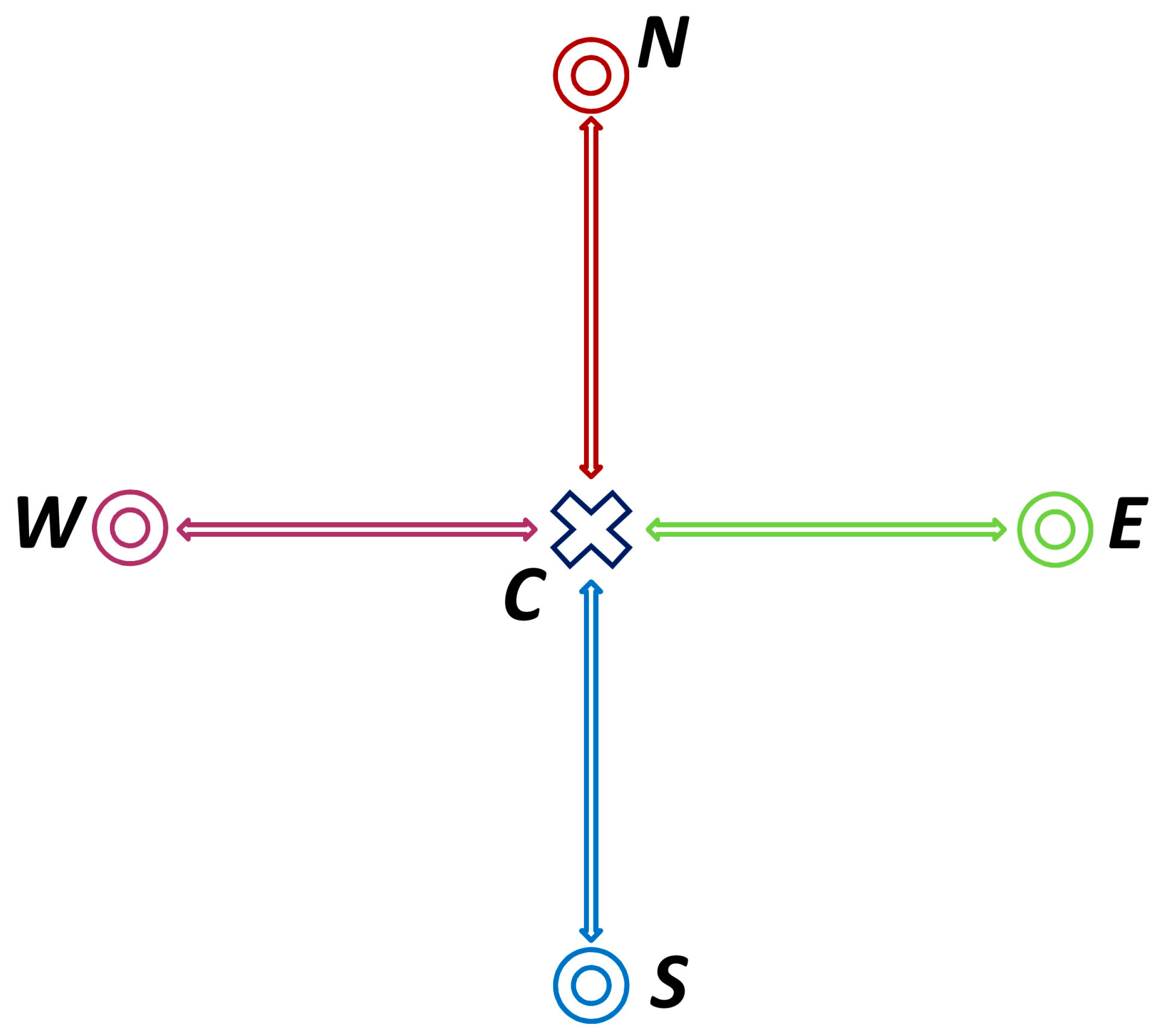
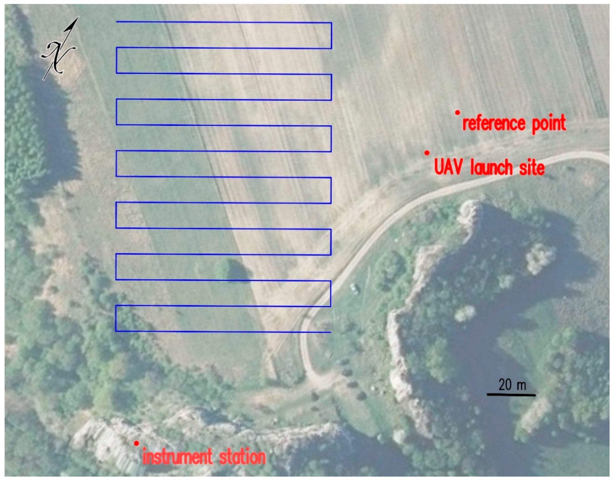
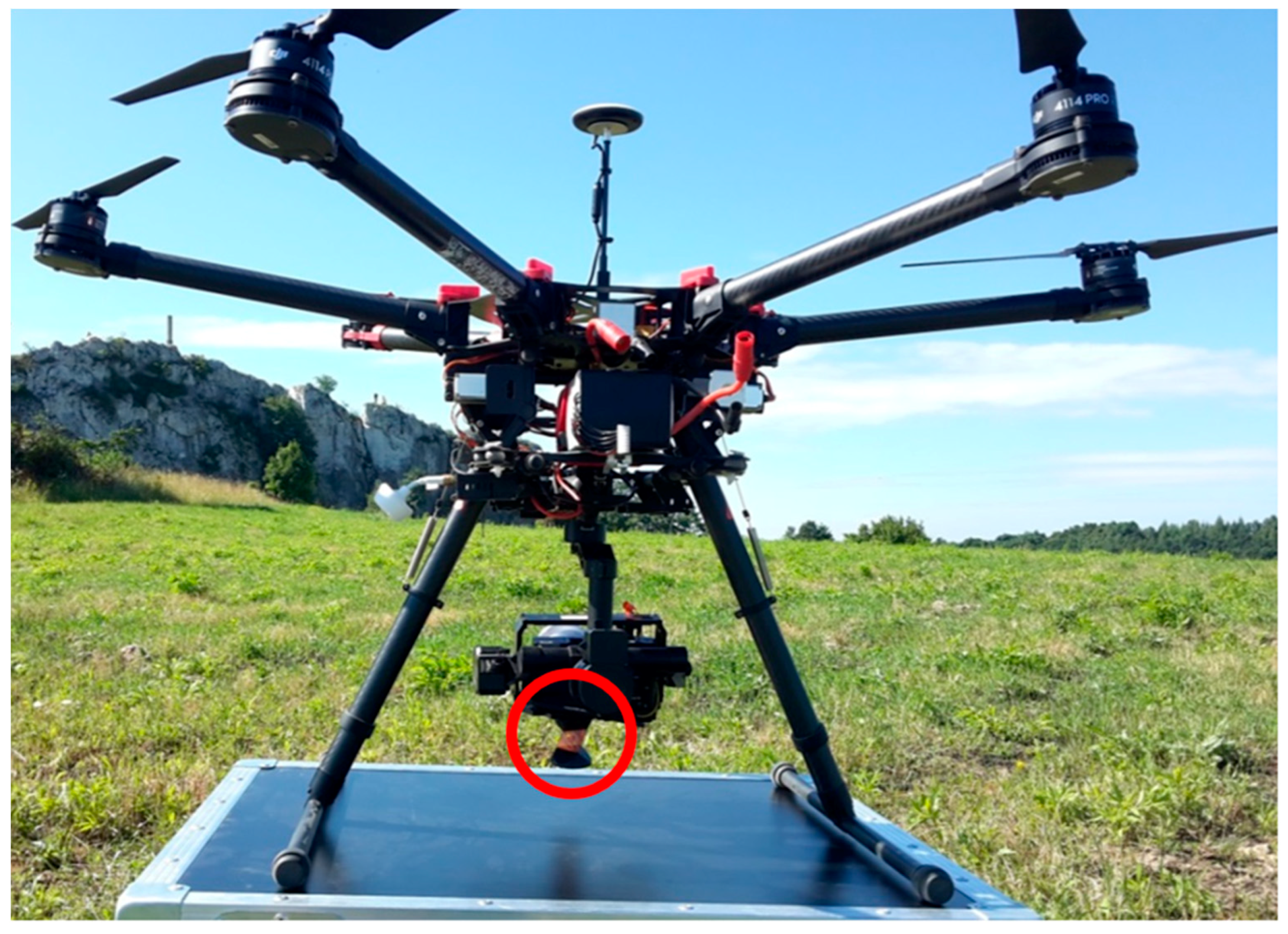
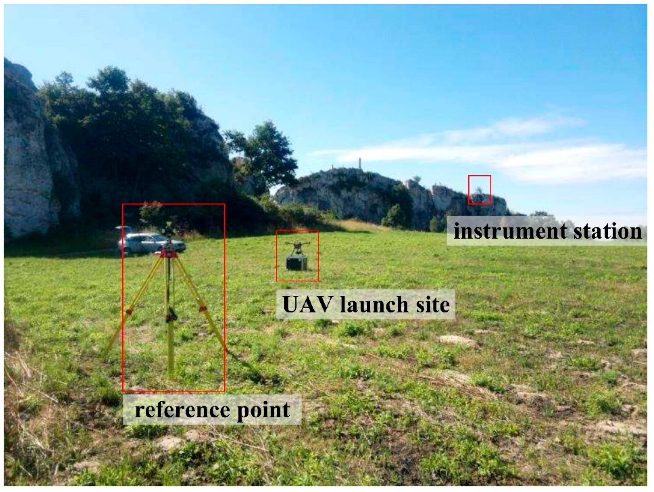
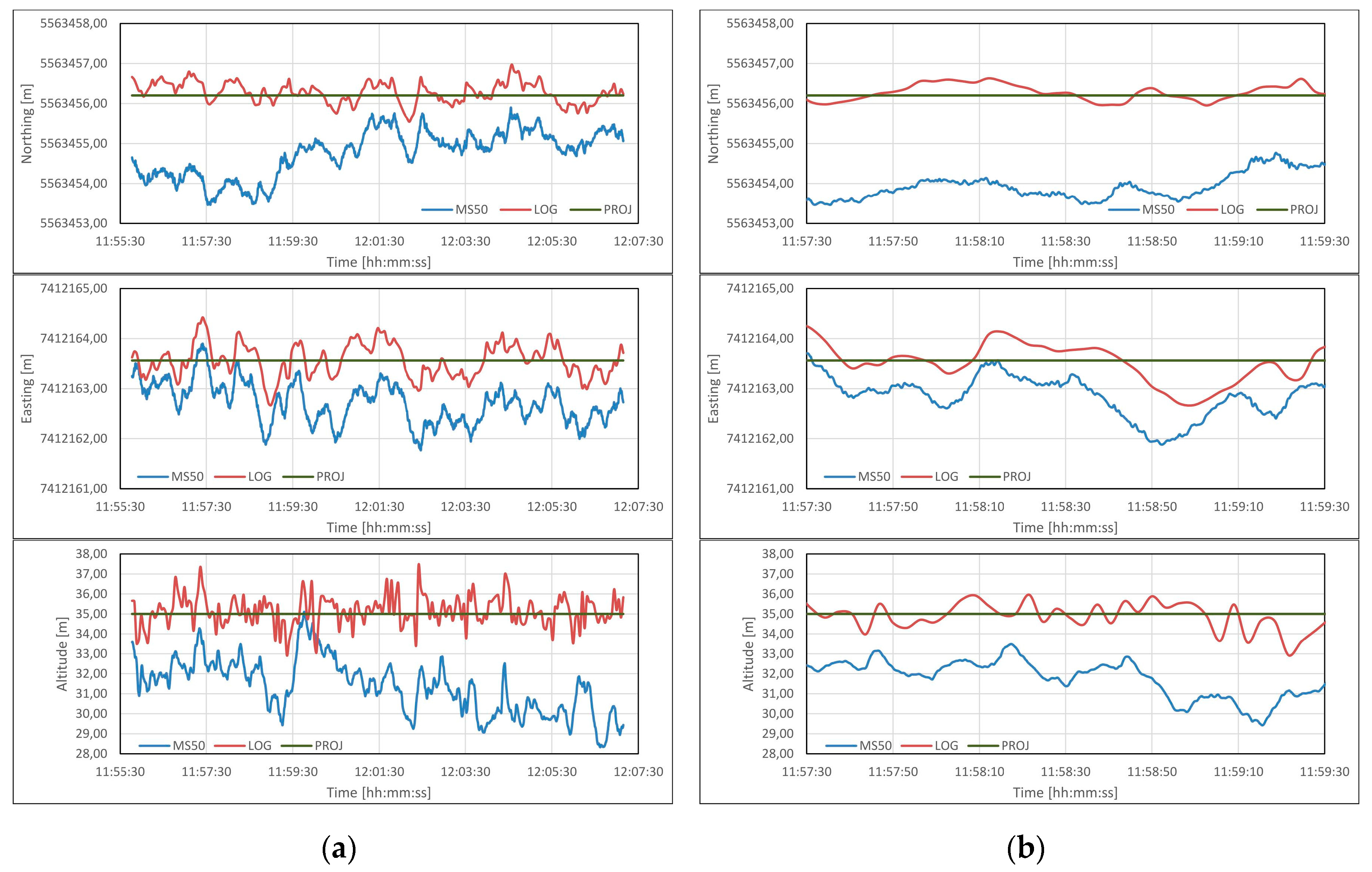
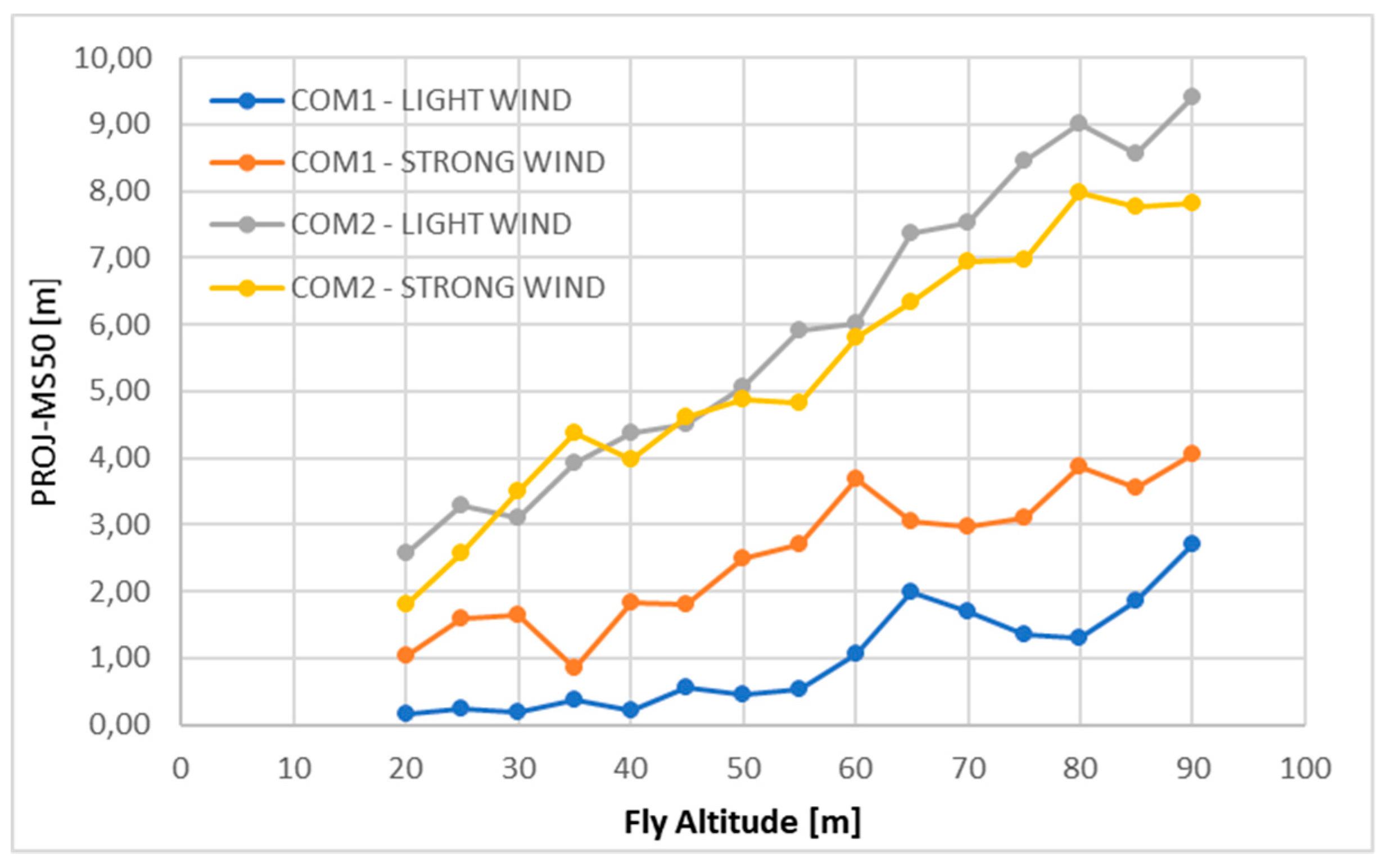
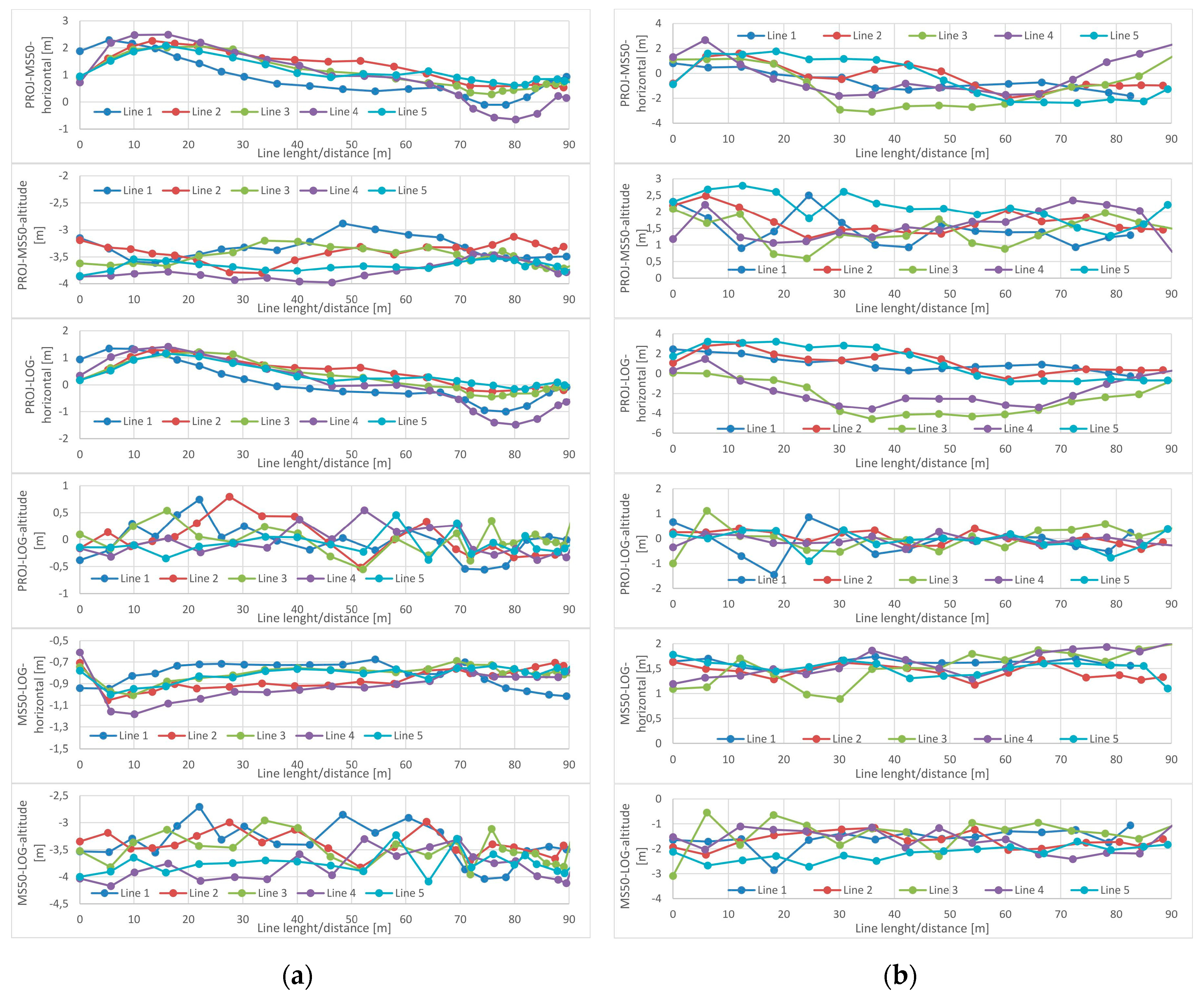
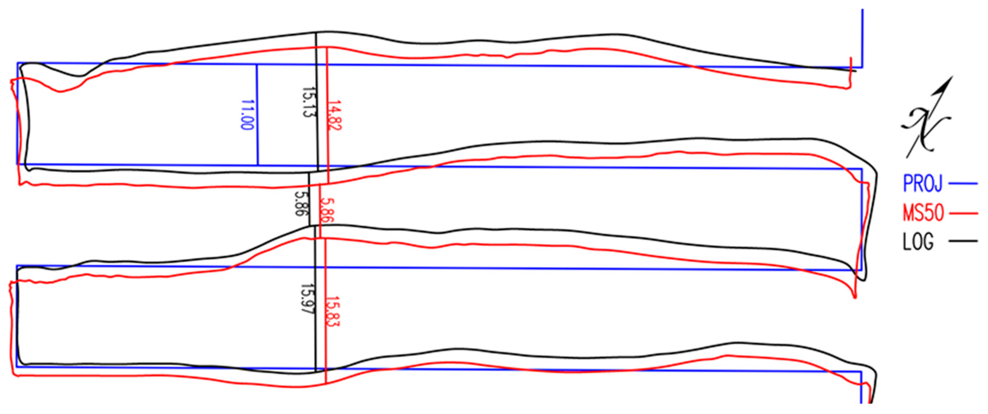
Table 1.
Values of maximum and minimum differences, their ranges and means, and standard deviations for individual data pairs in task 1.
Table 1.
Values of maximum and minimum differences, their ranges and means, and standard deviations for individual data pairs in task 1.
| PROJ-MS50 | PROJ-LOG | MS50-LOG | |||||||||
|---|---|---|---|---|---|---|---|---|---|---|---|
| N [m] | E [m] | A [m] | N [m] | E [m] | A [m] | N [m] | E [m] | A [m] | |||
| LIGHT WIND | COM-1 | MAX | 1.85 | 1.93 | 2.31 | 0.80 | 0.94 | 0.66 | −0.03 | 0.30 | −0.23 |
| MIN | 0.11 | −0.56 | 0.49 | −0.63 | −1.28 | −0.97 | −1.59 | −2.11 | −2.37 | ||
| MAX-MIN | 1.74 | 2.49 | 1.82 | 1.42 | 2.22 | 1.63 | 1.55 | 2.41 | 2.14 | ||
| 0.78 | 0.94 | 1.32 | −0.02 | 0.08 | −0.05 | −0.80 | −0.87 | −1.37 | |||
| σ | 0.30 | 0.48 | 0.36 | 0.25 | 0.42 | 0.28 | 0.25 | 0.41 | 0.40 | ||
| COM-2 | MAX | 2.15 | 1.54 | 5.57 | 0.64 | 1.00 | 1.09 | −1.24 | −0.20 | −3.23 | |
| MIN | 1.06 | −0.29 | 2.81 | −0.42 | −0.80 | −1.29 | −1.85 | −0.72 | −4.76 | ||
| MAX-MIN | 1.10 | 1.82 | 2.75 | 1.06 | 1.81 | 2.38 | 0.61 | 0.52 | 1.53 | ||
| 1.66 | 0.77 | 3.93 | 0.11 | 0.32 | −0.08 | −1.55 | −0.45 | −4.01 | |||
| σ | 0.23 | 0.35 | 0.65 | 0.22 | 0.35 | 0.54 | 0.11 | 0.12 | 0.37 | ||
| STRONG WIND | COM-1 | MAX | 2.60 | 1.62 | 3.86 | 0.79 | 0.86 | 0.74 | 0.62 | 1.60 | −2.38 |
| MIN | −0.40 | −0.85 | 2.39 | −0.86 | −1.07 | −0.60 | −2.80 | −2.02 | −4.17 | ||
| MAX-MIN | 3.00 | 2.47 | 1.47 | 1.66 | 1.93 | 1.33 | 3.42 | 3.62 | 1.79 | ||
| 1.17 | 0.44 | 3.22 | 0.05 | −0.04 | 0.02 | −1.12 | −0.48 | −3.20 | |||
| 0.77 | 0.58 | 0.25 | 0.31 | 0.40 | 0.27 | 0.79 | 0.69 | 0.38 | |||
| COM-2 | MAX | 2.70 | 1.77 | 6.67 | 0.66 | 0.89 | 2.07 | −0.68 | −0.18 | 0.48 | |
| MIN | 0.49 | 0.06 | 0.01 | −0.77 | −0.65 | −2.39 | −2.66 | −1.46 | −6.58 | ||
| MAX-MIN | 2.21 | 1.71 | 6.66 | 1.43 | 1.54 | 4.46 | 1.98 | 1.28 | 7.06 | ||
| 1.32 | 0.94 | 3.84 | −0.03 | 0.01 | −0.14 | −1.36 | −0.92 | −3.99 | |||
| 0.55 | 0.36 | 1.37 | 0.26 | 0.33 | 0.74 | 0.54 | 0.22 | 1.43 | |||
Table 2.
Values of time drifts calculated for all tests for each coordinate for data from MS50 and LOG in task 1.
Table 2.
Values of time drifts calculated for all tests for each coordinate for data from MS50 and LOG in task 1.
| MS50 | LOG | ||||||
|---|---|---|---|---|---|---|---|
| N [m/min] | E [m/min] | A [m/min] | N [m/min] | E [m/min] | A [m/min] | ||
| LIGHT WIND | COM-1 | 0.009 | 0.000 | −0.055 | −0.012 | 0.002 | 0.003 |
| COM-2 | −0.035 | −0.046 | −0.152 | 0.001 | −0.002 | 0.003 | |
| STRONG WIND | COM-1 | −0.187 | 0.116 | −0.057 | −0.013 | 0.015 | 0.002 |
| COM-2 | 0.130 | −0.057 | −0.278 | −0.021 | −0.007 | 0.010 | |
Table 3.
Results of UAV positioning accuracy test in task 2.
| Approach Direction | LIGHT WIND | STRONG WIND | |||||||
|---|---|---|---|---|---|---|---|---|---|
| N [m] | E [m] | A [m] | 3D [m] | N [m] | E [m] | A [m] | 3D [m] | ||
| COM-1 | N | 0.76 | −0.68 | −1.79 | 2.06 | −1.10 | 0.55 | −2.11 | 2.44 |
| S | 0.98 | −0.53 | −1.66 | 2.00 | −1.65 | 0.21 | −2.57 | 3.06 | |
| E | 0.86 | −0.90 | −1.81 | 2.20 | −1.33 | 0.36 | −2.75 | 3.08 | |
| W | 0.50 | −0.55 | −2.24 | 2.36 | −1.80 | 0.47 | −2.15 | 2.84 | |
| COM-2 | N | 1.59 | 0.03 | −1.99 | 2.55 | 0.69 | −0.68 | −2.50 | 2.68 |
| S | 1.50 | 0.96 | −1.70 | 2.46 | 0.99 | −0.94 | −2.70 | 3.02 | |
| E | 0.50 | −0.19 | −1.35 | 1.45 | 0.43 | −0.13 | −3.69 | 3.71 | |
| W | 1.66 | 0.69 | −1.29 | 2.21 | 0.74 | −0.62 | −3.05 | 3.20 | |
Table 4.
Results of positioning repeatability test and variability of positioning accuracy test from many directions of UAV approach in task 2.
Table 4.
Results of positioning repeatability test and variability of positioning accuracy test from many directions of UAV approach in task 2.
| Approach Direction | N [m] | S [m] | E [m] | W [m] | vAPP [m] | |
|---|---|---|---|---|---|---|
| LIGHT WIND | COM-1 | 1.83 | 1.58 | 2.30 | 1.75 | 0.91 |
| COM-2 | 0.63 | 1.25 | 1.00 | 0.54 | 0.66 | |
| STRONG WIND | COM-1 | 2.41 | 2.19 | 2.51 | 2.79 | 1.17 |
| COM-2 | 2.86 | 2.31 | 2.40 | 2.96 | 1.57 | |
Table 5.
Results of distance deviation test and repeatability test of the implemented distance in task 2.
Table 5.
Results of distance deviation test and repeatability test of the implemented distance in task 2.
| Deviation of the Distance | Repeatability of the Distance | ||||||||||
|---|---|---|---|---|---|---|---|---|---|---|---|
| N [m] | S [m] | E [m] | W [m] | N [m] | S [m] | E [m] | W [m] | ||||
| LIGHT WIND | COM-1 | −0.27 | −0.50 | −0.33 | −0.57 | −0.42 | 0.88 | 1.11 | 1.07 | 0.97 | 1.01 |
| COM-2 | −0.81 | −0.25 | −0.49 | −0.67 | −0.56 | 0.84 | 1.19 | 0.92 | 1.08 | 1.01 | |
| STRONG WIND | COM-1 | −0.33 | −0.54 | −0.46 | −0.32 | −0.41 | 1.58 | 1.44 | 1.31 | 1.37 | 1.43 |
| COM-2 | −0.37 | −0.60 | −0.85 | −0.67 | −0.62 | 1.51 | 1.31 | 1.43 | 1.03 | 1.32 | |
Table 6.
Results of task 3: design altitudes and differences calculated for MS50, LOG, and PROJ data.
Table 6.
Results of task 3: design altitudes and differences calculated for MS50, LOG, and PROJ data.
| LIGHT WIND | STRONG WIND | ||||||||
|---|---|---|---|---|---|---|---|---|---|
| Designed Altitude [m] | PROJ-MS50 [m] | PROJ-LOG [m] | MS50-LOG [m] | Scale | PROJ-MS50 [m] | PROJ-LOG [m] | MS50-LOG [m] | Scale | |
| COM-1 | 20 | 0.15 | −0.28 | −0.44 | 0.99 | 1.05 | −0.12 | −1.17 | 0.95 |
| 25 | 0.25 | −0.30 | −0.55 | 0.99 | 1.61 | 0.51 | −1.10 | 0.94 | |
| 30 | 0.20 | 0.11 | −0.09 | 0.99 | 1.65 | −0.26 | −1.91 | 0.94 | |
| 35 | 0.36 | −0.03 | −0.39 | 0.99 | 0.85 | −0.61 | −1.46 | 0.98 | |
| 40 | 0.22 | −0.17 | −0.39 | 0.99 | 1.82 | 0.33 | −1.50 | 0.95 | |
| 45 | 0.55 | 0.00 | −0.55 | 0.99 | 1.81 | −0.58 | −2.39 | 0.96 | |
| 50 | 0.46 | −0.17 | −0.63 | 0.99 | 2.50 | −0.06 | −2.57 | 0.95 | |
| 55 | 0.53 | −0.16 | −0.69 | 0.99 | 2.70 | −0.25 | −2.95 | 0.95 | |
| 60 | 1.07 | −0.14 | −1.21 | 0.98 | 3.69 | 0.01 | −3.68 | 0.94 | |
| 65 | 1.99 | 0.24 | −1.74 | 0.97 | 3.05 | −0.46 | −3.51 | 0.95 | |
| 70 | 1.70 | −0.22 | −1.93 | 0.98 | 2.97 | −0.38 | −3.35 | 0.96 | |
| 75 | 1.35 | −0.07 | −1.42 | 0.98 | 3.10 | 0.17 | −2.93 | 0.96 | |
| 80 | 1.29 | −0.29 | −1.59 | 0.98 | 3.87 | 0.03 | −3.84 | 0.95 | |
| 85 | 1.85 | −0.20 | −2.06 | 0.98 | 3.55 | −0.45 | −4.00 | 0.96 | |
| 90 | 2.70 | −0.26 | −2.96 | 0.97 | 4.07 | 0.12 | −3.94 | 0.95 | |
| COM-2 | 20 | 2.57 | −0.37 | −2.95 | 0.87 | 1.81 | 0.05 | −1.76 | 0.91 |
| 25 | 3.30 | −0.22 | −3.52 | 0.87 | 2.56 | 0.28 | −2.28 | 0.90 | |
| 30 | 3.11 | −0.29 | −3.40 | 0.90 | 3.50 | −0.07 | −3.57 | 0.88 | |
| 35 | 3.92 | −0.14 | −4.05 | 0.89 | 4.37 | −0.05 | −4.42 | 0.88 | |
| 40 | 4.39 | −0.46 | −4.84 | 0.89 | 3.97 | −0.32 | −4.30 | 0.90 | |
| 45 | 4.51 | −0.74 | −5.25 | 0.90 | 4.61 | 0.22 | −4.39 | 0.90 | |
| 50 | 5.05 | −0.30 | −5.35 | 0.90 | 4.88 | −0.32 | −5.20 | 0.90 | |
| 55 | 5.92 | 0.32 | −5.60 | 0.89 | 4.81 | 0.14 | −4.67 | 0.91 | |
| 60 | 6.03 | 0.93 | −5.09 | 0.90 | 5.82 | 0.00 | −5.82 | 0.90 | |
| 65 | 7.37 | 0.07 | −7.30 | 0.89 | 6.33 | −0.05 | −6.38 | 0.90 | |
| 70 | 7.54 | 0.93 | −6.61 | 0.89 | 6.95 | −0.38 | −7.33 | 0.90 | |
| 75 | 8.45 | −0.06 | −8.50 | 0.89 | 6.96 | −0.20 | −7.16 | 0.91 | |
| 80 | 9.02 | 0.33 | −8.68 | 0.89 | 7.97 | −0.69 | −8.66 | 0.90 | |
| 85 | 8.55 | −0.63 | −9.18 | 0.90 | 7.77 | −0.24 | −8.01 | 0.91 | |
| 90 | 9.42 | −0.53 | −9.95 | 0.90 | 7.83 | −0.54 | −8.37 | 0.91 | |
Table 7.
Values of correlation between designed altitudes and differences resulting from measurements using a given method in task 3.
Table 7.
Values of correlation between designed altitudes and differences resulting from measurements using a given method in task 3.
| PROJ-MS50 | PROJ-LOG | MS50-LOG | ||
|---|---|---|---|---|
| LIGHT WIND | COM-1 | 0.90 | 0.11 | 0.90 |
| COM-2 | 0.99 | 0.21 | 0.97 | |
| STRONG WIND | COM-1 | 0.93 | 0.06 | 0.94 |
| COM-2 | 0.98 | 0.16 | 0.98 |
Table 8.
Values of maximum and minimum increments between flight levels, their mean values, and standard deviation of these values in task 4.
Table 8.
Values of maximum and minimum increments between flight levels, their mean values, and standard deviation of these values in task 4.
| Designed | COM-1 LIGHT WIND | COM-2 LIGHT WIND | COM-1 STRONG WIND | COM-2 STRONG WIND | |||||
|---|---|---|---|---|---|---|---|---|---|
| Measured Increments | |||||||||
| Start Altitude [m] | End Altitude [m] | MS50 [m] | LOG [m] | MS50 [m] | LOG [m] | MS50 [m] | LOG [m] | MS50 [m] | LOG [m] |
| 20 | 25 | 4.91 | 5.02 | 4.27 | 4.85 | 4.44 | 4.38 | 4.24 | 4.77 |
| 25 | 30 | 5.05 | 4.60 | 5.19 | 5.07 | 4.95 | 5.77 | 4.06 | 5.35 |
| 30 | 35 | 4.83 | 5.13 | 4.19 | 4.85 | 5.80 | 5.35 | 4.13 | 4.98 |
| 35 | 40 | 5.15 | 5.15 | 4.53 | 5.32 | 4.03 | 4.07 | 5.40 | 5.28 |
| 40 | 45 | 4.66 | 4.82 | 4.87 | 5.28 | 5.01 | 5.91 | 4.36 | 4.45 |
| 45 | 50 | 5.09 | 5.18 | 4.46 | 4.56 | 4.30 | 4.48 | 4.73 | 5.54 |
| 50 | 55 | 4.93 | 4.99 | 4.13 | 4.38 | 4.81 | 5.19 | 5.07 | 4.54 |
| 55 | 60 | 4.46 | 4.97 | 4.89 | 4.39 | 4.01 | 4.74 | 4.00 | 5.14 |
| 60 | 65 | 4.08 | 4.62 | 3.66 | 5.86 | 5.64 | 5.47 | 4.49 | 5.05 |
| 65 | 70 | 5.28 | 5.46 | 4.83 | 4.15 | 5.08 | 4.92 | 4.38 | 5.33 |
| 70 | 75 | 5.35 | 4.85 | 4.10 | 5.99 | 4.87 | 4.45 | 4.99 | 4.81 |
| 75 | 80 | 5.06 | 5.23 | 4.43 | 4.61 | 4.23 | 5.14 | 3.99 | 5.49 |
| 80 | 85 | 4.44 | 4.91 | 5.47 | 5.97 | 5.32 | 5.48 | 5.21 | 4.55 |
| 85 | 90 | 4.15 | 5.05 | 4.13 | 4.89 | 4.49 | 4.43 | 4.94 | 5.30 |
| MAX | 5.35 | 5.46 | 5.47 | 5.99 | 5.80 | 5.91 | 5.40 | 5.54 | |
| MIN | 4.08 | 4.60 | 3.66 | 4.15 | 4.01 | 4.07 | 3.99 | 4.45 | |
| MAX-MIN | 1.27 | 0.87 | 1.81 | 1.84 | 1.79 | 1.84 | 1.41 | 1.09 | |
| 4.82 | 5.00 | 4.51 | 5.01 | 4.78 | 4.98 | 4.57 | 5.04 | ||
| σ | 0.40 | 0.23 | 0.49 | 0.60 | 0.56 | 0.57 | 0.48 | 0.36 | |
Table 9.
Values of maximum and minimum distances from designed flight lines in task 4.
| PROJ-MS50 | PROJ-LOG | MS50-LOG | ||||||
|---|---|---|---|---|---|---|---|---|
| p [m] | A [m] | p [m] | A [m] | p [m] | A [m] | |||
| LIGHT WIND | COM-1 | MAX | 2.04 | 2.10 | 1.61 | 0.77 | 1.82 | 2.43 |
| MIN | −1.69 | 0.31 | −0.91 | −1.13 | −1.19 | 0.29 | ||
| MAX-MIN | 3.73 | 1.80 | 2.52 | 1.90 | 3.01 | 2.14 | ||
| −0.05 | 1.31 | 0.08 | −0.01 | 0.26 | 1.32 | |||
| 0.90 | 0.46 | 0.48 | 0.41 | 0.67 | 0.49 | |||
| COM-2 | MAX | 2.49 | 2.87 | 1.41 | 0.80 | 1.02 | 2.51 | |
| MIN | −1.51 | 4.14 | −1.48 | −0.56 | −1.18 | 4.17 | ||
| MAX-MIN | 4.01 | 1.27 | 2.89 | 1.35 | 2.20 | 1.67 | ||
| 0.20 | 3.54 | 0.13 | −0.04 | −0.05 | 3.58 | |||
| σ | 1.00 | 0.23 | 0.52 | 0.23 | 0.78 | 0.30 | ||
| STRONG WIND | COM-1 | MAX | 2.68 | 3.17 | 3.24 | 1.11 | 2.02 | 0.23 |
| MIN | −3.26 | 0.44 | −4.62 | −1.45 | −1.75 | −3.13 | ||
| MAX-MIN | 5.94 | 2.73 | 7.86 | 2.56 | 3.77 | 3.36 | ||
| −0.23 | 1.66 | −0.16 | 0.00 | 1.27 | −1.67 | |||
| 1.41 | 0.54 | 2.06 | 0.43 | 0.91 | 0.54 | |||
| COM-2 | MAX | 2.22 | 5.25 | 1.15 | 0.91 | 1.61 | −2.75 | |
| MIN | −2.15 | 2.07 | −1.08 | −1.36 | −1.66 | −5.53 | ||
| MAX-MIN | 4.37 | 3.18 | 2.24 | 2.27 | 3.27 | 2.78 | ||
| 0.26 | 3.77 | 0.24 | −0.06 | −0.04 | −3.84 | |||
| σ | 1.45 | 0.63 | 0.50 | 0.45 | 1.14 | 0.58 | ||
Table 10.
Values of maximum and minimum differences, their ranges as well as mean and standard deviations for individual data pairs in task 4.
Table 10.
Values of maximum and minimum differences, their ranges as well as mean and standard deviations for individual data pairs in task 4.
| PROJ-MS50 | PROJ-LOG | MS50-LOG | |||||||||
|---|---|---|---|---|---|---|---|---|---|---|---|
| N [m] | E [m] | A [m] | N [m] | E [m] | A [m] | N [m] | E [m] | A [m] | |||
| LIGHT WIND | COM-1 | MAX | 2.93 | 2.00 | 3.92 | 1.52 | 2.32 | 0.77 | −0.43 | 0.55 | −1.89 |
| MIN | 0.95 | 0.34 | 1.90 | −0.40 | −0.62 | −1.13 | −1.83 | −1.74 | −3.75 | ||
| MAX-MIN | 1.99 | 1.66 | 2.02 | 1.92 | 2.94 | 1.90 | 1.40 | 2.29 | 1.86 | ||
| 1.70 | 1.09 | 2.90 | 0.62 | 0.48 | −0.23 | −1.09 | −0.61 | −3.13 | |||
| σ | 0.59 | 0.57 | 0.70 | 0.58 | 1.19 | 0.49 | 0.46 | 0.81 | 0.57 | ||
| COM-2 | MAX | 0.02 | 0.75 | 3.99 | 0.13 | 0.70 | 0.26 | 1.09 | 0.25 | −3.02 | |
| MIN | −1.65 | −0.56 | 2.87 | −1.05 | −0.45 | −0.38 | −0.24 | −0.74 | −4.13 | ||
| MAX-MIN | 1.66 | 1.31 | 1.12 | 1.18 | 1.15 | 0.64 | 1.33 | 0.98 | 1.11 | ||
| −0.84 | 0.18 | 3.53 | −0.48 | 0.11 | −0.11 | 0.36 | −0.07 | −3.64 | |||
| 0.41 | 0.34 | 0.29 | 0.36 | 0.40 | 0.20 | 0.43 | 0.35 | 0.31 | |||
| STRONG WIND | COM-1 | MAX | 2.97 | 0.18 | 2.40 | 0.84 | 0.42 | 0.39 | −1.43 | 0.24 | −0.66 |
| MIN | 0.28 | −1.36 | 0.33 | −1.49 | −1.70 | −1.00 | −2.34 | −0.59 | −2.24 | ||
| MAX-MIN | 2.69 | 1.54 | 2.07 | 2.33 | 2.12 | 1.39 | 0.91 | 0.83 | 1.58 | ||
| 1.72 | −0.61 | 1.18 | −0.06 | −0.67 | −0.25 | −1.78 | −0.06 | −1.43 | |||
| σ | 0.77 | 0.51 | 0.50 | 0.63 | 0.64 | 0.45 | 0.27 | 0.23 | 0.45 | ||
| COM-2 | MAX | 2.37 | 0.96 | 4.38 | 0.50 | 0.36 | 0.86 | −1.38 | −0.01 | −2.63 | |
| MIN | 1.03 | 0.20 | 2.33 | −0.61 | −0.80 | −0.80 | −2.16 | −1.48 | −4.53 | ||
| MAX-MIN | 1.34 | 0.76 | 2.06 | 1.11 | 1.17 | 1.67 | 0.78 | 1.47 | 1.90 | ||
| 1.68 | 0.63 | 3.66 | 0.02 | −0.17 | −0.05 | −1.66 | −0.79 | −3.71 | |||
| σ | 0.47 | 0.24 | 0.65 | 0.32 | 0.51 | 0.47 | 0.25 | 0.60 | 0.53 | ||
Table 11.
Values of distances to the ends of mission flight lines (maximum, minimum, their ranges, mean values, and standard deviations) for data in task 5.
Table 11.
Values of distances to the ends of mission flight lines (maximum, minimum, their ranges, mean values, and standard deviations) for data in task 5.
| LIGHT WIND | STRONG WIND | ||||||
|---|---|---|---|---|---|---|---|
| PROJ-MS [m] | PROJ-LOG [m] | MS-LOG [m] | PROJ-MS [m] | PROJ-LOG [m] | MS-LOG [m] | ||
| COM-1 | MAX | 10.07 | 10.18 | 0.61 | 10.19 | 10.22 | 0.76 |
| MIN | 8.44 | 8.97 | 0.27 | 8.56 | 9.08 | 0.41 | |
| MAX-MIN | 1.64 | 1.21 | 0.34 | 1.63 | 1.14 | 0.35 | |
| 9.33 | 9.68 | 0.44 | 9.37 | 9.54 | 0.58 | ||
| σ | 0.50 | 0.37 | 0.10 | 0.81 | 0.61 | 0.18 | |
| COM-2 | MAX | 9.77 | 10.30 | 0.61 | 10.47 | 10.46 | 0.98 |
| MIN | 8.66 | 9.09 | 0.46 | 8.67 | 9.04 | 0.11 | |
| MAX-MIN | 1.11 | 1.21 | 0.15 | 1.80 | 1.42 | 0.87 | |
| 9.14 | 9.64 | 0.54 | 9.48 | 9.64 | 0.51 | ||
| 0.41 | 0.42 | 0.06 | 0.91 | 0.57 | 0.44 | ||
Table 12.
Values of image coverage changes depending on changes in the distance between flight lines.
Table 12.
Values of image coverage changes depending on changes in the distance between flight lines.
| Changes in Distances between Flight Lines [m] | Image Width [m] | ||||||
|---|---|---|---|---|---|---|---|
| 40 | 60 | 80 | 100 | 150 | 200 | 300 | |
| 0.00 | 60.0% | 60.0% | 60.0% | 60.0% | 60.0% | 60.0% | 60.0% |
| 2.50 | 53.8% | 55.8% | 56.9% | 57.5% | 58.3% | 58.8% | 59.2% |
| 5.00 | 47.5% | 51.7% | 53.8% | 55.0% | 56.7% | 57.5% | 58.3% |
| 10.00 | 35.0% | 43.3% | 47.5% | 50.0% | 53.3% | 55.0% | 56.7% |
Table 13.
Values of image coverage changes depending on changes in flying altitudes and focal length.
Table 13.
Values of image coverage changes depending on changes in flying altitudes and focal length.
| GSD [mm] | Change of Flying Altitude [m] | Focal Length | |||||
|---|---|---|---|---|---|---|---|
| 15 mm | 15 mm | 25 mm | 25 mm | 40 mm | 40 mm | ||
| 10 | 0.0 | 60.0% | 80.0% | 60.0% | 80.0% | 60.0% | 80.0% |
| 2.5 | 57.3% | 78.6% | 58.4% | 79.2% | 59.0% | 79.5% | |
| 5.0 | 54.1% | 77.1% | 56.7% | 78.3% | 58.0% | 79.0% | |
| 10.0 | 46.1% | 73.0% | 52.7% | 76.3% | 55.7% | 77.9% | |
| 20 | 0.0 | 60.0% | 80.0% | 60.0% | 80.0% | 60.0% | 80.0% |
| 2.5 | 58.7% | 79.4% | 59.2% | 79.6% | 59.5% | 79.8% | |
| 5.0 | 57.3% | 78.6% | 58.4% | 79.2% | 59.0% | 79.5% | |
| 10.0 | 54.1% | 77.1% | 56.7% | 78.3% | 58.0% | 79.0% | |
| 30 | 0.0 | 60.0% | 80.0% | 60.0% | 80.0% | 60.0% | 80.0% |
| 2.5 | 59.1% | 79.6% | 59.5% | 79.7% | 59.7% | 79.8% | |
| 5.0 | 58.2% | 79.1% | 58.9% | 79.5% | 59.3% | 79.7% | |
| 10.0 | 56.2% | 78.1% | 57.8% | 78.9% | 58.7% | 79.3% | |
© 2019 by the author. Licensee MDPI, Basel, Switzerland. This article is an open access article distributed under the terms and conditions of the Creative Commons Attribution (CC BY) license (http://creativecommons.org/licenses/by/4.0/).
Share and Cite
MDPI and ACS Style
Ćwiąkała, P. Testing Procedure of Unmanned Aerial Vehicles (UAVs) Trajectory in Automatic Missions. Appl. Sci. 2019, 9, 3488. https://0-doi-org.brum.beds.ac.uk/10.3390/app9173488
AMA Style
Ćwiąkała P. Testing Procedure of Unmanned Aerial Vehicles (UAVs) Trajectory in Automatic Missions. Applied Sciences. 2019; 9(17):3488. https://0-doi-org.brum.beds.ac.uk/10.3390/app9173488
Chicago/Turabian StyleĆwiąkała, Paweł. 2019. "Testing Procedure of Unmanned Aerial Vehicles (UAVs) Trajectory in Automatic Missions" Applied Sciences 9, no. 17: 3488. https://0-doi-org.brum.beds.ac.uk/10.3390/app9173488
Note that from the first issue of 2016, this journal uses article numbers instead of page numbers. See further details here.