1. Introduction
Nowadays, due to a rapid development of global navigation satellite system (GNSS) [
1] the problem of rail routes reconstruction in a global reference system turns out to be increasingly possible. Knowing the coordinates of longitudinal track centerline, it is possible to work with so called Absolute Track Geometry. The essence of the process is determining the axis of railway tracks in the form Cartesian coordinates of a global or local coordinate system. The pioneering studies with a use of satellite measurements on railway tracks using a mobile measuring trolley were conducted in the 1990s at the University of Graz in cooperation with the Plasser & Theurer company [
2]. In the early 2000s, a research on the application of precise GNSS measurements to determine track position was conducted at Marshall University [
3]. Since then, the mobile measurements and analysis of real time kinematic data (RTK) have been developed by researchers and engineers. The current methods being developed for determining coordinates using GNSS techniques allow engineers for an accurate survey of a railway or tram tracks in a practical and economically effective manner [
3,
4,
5,
6,
7,
8,
9].
In 2009, an interdisciplinary scientific team of the Gdansk University of Technology, Gdynia Maritime University, and Polish Naval Academy joined to this investigations and started to develop a method for mobile measurements of a track centerline [
10,
11,
12,
13,
14,
15,
16]. The method was called a mobile satellite measurement (MSM) method, which included typical solutions, like differential global positioning system (DGPS) and RTK, but also original measurement data processing algorithms adapted for railway geometry specifics. From the beginning, it was certain that the accuracy of obtained track positions is significantly affected by a horizontal shift of the antennas centres in relation to the track axis. That occurs while the platform runs through circular curves and transition curves. This shift results from the tilting of the measuring platform due to the rail height differences, the so-called cant, which is commonly constructed on the length of these track sections. So, the lack of compensation for the measurement signal results with an inaccuracy in the identification of the track absolute geometry.
Although the earlier work of the authors took into account the influence of the track cant on the measurements and the estimation of the track axis coordinates, the corrections have been determined with the knowledge of the track inclination value from independent measurements [
17]. This means that the relevant corrections were calculated based on the cant measurements conducted by the methods commonly used in diagnostics and maintenance of the railway track.
A subject matter of data fusion of inertial navigation system (INS) and GNSS signals have been discussed for example in papers [
3,
4,
5,
9]. The algorithms currently presented in the literature are often based on the data-fusion process using Kalman filters [
4,
9]. This data fusion is commonly implemented for combining the GNSS and INS signals, especially when the quality of GNSS is disturbed by terrestrial obstacles or even when the signal is interrupted (i.e., in tunnels or under viaducts). On the other hand, INS is subject to the control of the GNSS signal, especially to avoid the influence of drift.
Such redundancy certainly improves reliability of the measurement system [
3]. In this paper, the integration of INS and GNSS signals is focused on the previously mention problem, i.e., on calculating the corrections for a track inclination impact on the measured positions. However, the integration of both measurements into the multisensory platform results in an increase of measurement efficiency, and therefore makes the entire process faster and cheaper.
Also, a crucial issue in such measurements is to improve the quality of track axis identification in a sense of measurement speed. Therefore, the possibilities to increase the speed in relation to devices pushed along the track, with a speed of about 5 km/h—to a speed of 30–60 km/h, are consequently tested. It is very important to keep a final accuracy in the range of 1–2 cm what is sufficient for problems related to the maintenance or design the geometric layout. So, the research target of the authors is to increase the accuracy along the measurement speed increase, from 5–10 km/h to 30–60 km/h range.
2. Materials and Methods
2.1. Track Position Measurements
Track axis identification in approach of absolute geometry have been realized with a use of MSM method by using RTK positioning with a run speed around 30-60 km/h. Track positions were recorded using 20 Hz position update rate, depending on a run velocity, in about 0.3 m step [
18,
19]. Considering the length between measured points, it is possible to increase the ran speed, especially, when the geometric sections are long (tangent and curve sections). It should be emphasized that increased run speed affects the inertial measurements due to a stronger impact of centrifugal effects when curvature on a track exist.
In order to analyze the possibilities of the cant distribution estimation on the base of inertial measurements, the authors developed a method for the estimation of this inclination. The algorithm was adopted to the GNSS track surveying. The measurements were conducted on Gdansk tramway network. As a pulling vehicle, the N8C-MF01 tram was used. The pre-war DWF 300 tram boogies were used as measuring platforms [
12]. That solution met the criteria for the track shape restoration because the antennas were fixed relatively close to the track level.
The measurement system recorded signals and information about following parameters:
Measurement performance date and time,
Geodetic coordinates of the measuring point (plane coordinates in the local coordinate system),
2D and 3D position uncertainty radius,
Number of satellites visible on the horizon,
Space system geometry,
Coordinate determination method (code, phase).
2.2. The Cant Estimation Method
The cant is one of the most important design parameters on railway and tram lines. It is defined as a difference of rails elevation in a particular track cross section. Along the circular part of arc the nominal cant value is constant, while in adjacent parts the cant value changes. These sections of differ cant value are called cant transitions [
20]. On curves with a cant, it is possible to achieve higher speeds, because a resultant value of centrifugal acceleration is lower. Therefore, even on high speed railways, the horizontal arcs are designed with a cant and cant transitions between arcs and tangents.
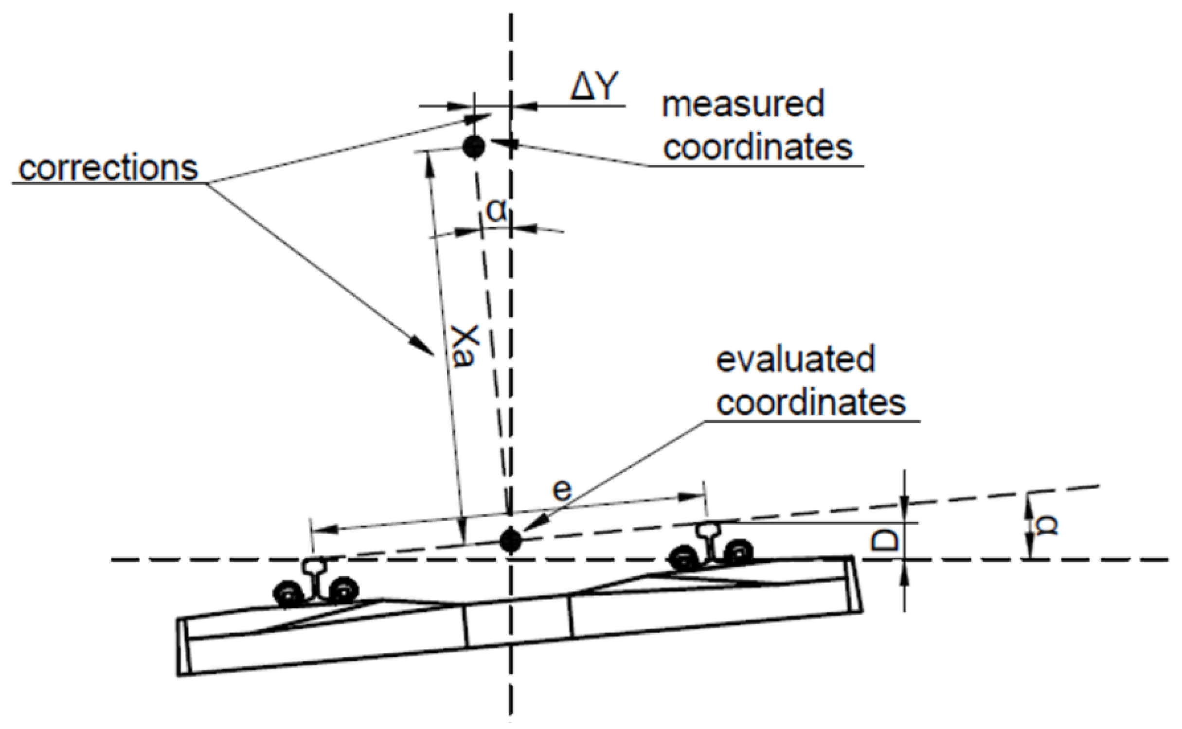
From a point of view of presented measurements, cant affects the accuracy of positioning the track axis in the horizontal plane what is shown in
Figure 1. Therefore, the measured coordinates should be corrected by taking into account a transverse shift. The correction of this shift is calculated according following Formula: [
21]:
where:
- ∆Y
– Transverse correction [mm],
- e
– Centreline spacing of the rails [mm],
- D
– Cant [mm],
- Xa
– Measuring device mounting height [mm].
The most commonly used method of cant determination is a static measurement using a manual gauge which is equipped with a level or inclinometer. Such a device is calibrated to allow a directly reading the cant in millimeters. The second common method is based on dynamic measurements and is used in measuring trolleys or trains [
1,
3,
4,
9,
11]. Due to additional accelerations and dynamic effects which affect the measurement during the vehicle run, the effective inertial measurement is relatively difficult. Therefore, to determine the cant, the measuring vehicles for railway track inventory are equipped mainly with advanced gyroscopes. There are two common types of gyros:
Gyrostat, consisting of rotating elements which retain their original position using the gyro effect. With such a device, it is possible to directly determine the angle of rotation of the gyro casing [
22].
Inertial Measurement Unit (IMU), consisting of a group of microelectromechanical systems (MEMS) of electromechanical accelerometers that determine the rotational speed of the device. The calculation of the integral is required to specify the angle of the IMU casing rotation:
where:
- α
– Vehicle’s angle of inclination in relation to the plane [rad],
- t
– Time [s],
- ω
– Angular velocity [rad/s].
Gyroscopic measurements have one fundamental disadvantage: the measurement result is dependent on the previous condition of the device, because the angle of rotation is not measured regarding to the global reference system, but to the earlier position of the gyro itself. For this reason, the device must be calibrated before measurement, but the measurement error increases with the test time [
23,
24,
25]. Therefore, in many standards for railways, the requirements for cant determination are not strict (accuracy within 5 mm) [
26,
27,
28]. The main disadvantage of a gyroscope is a drift, i.e., a systematic measurement error involving the accumulation of the measurement‘s result and a certain value (offset or bias) [
29,
30]. The offsets can also change over time. Therefore, the value obtained from the gyroscope should be considered as a resultant value of such components as:
where:
- ω
– Actual angular velocity [rad/s],
- ωg
– Angular velocity read from the gyroscope [rad/s],
- ωd
– Drift [rad/s],
- W
– White noise [rad/s].
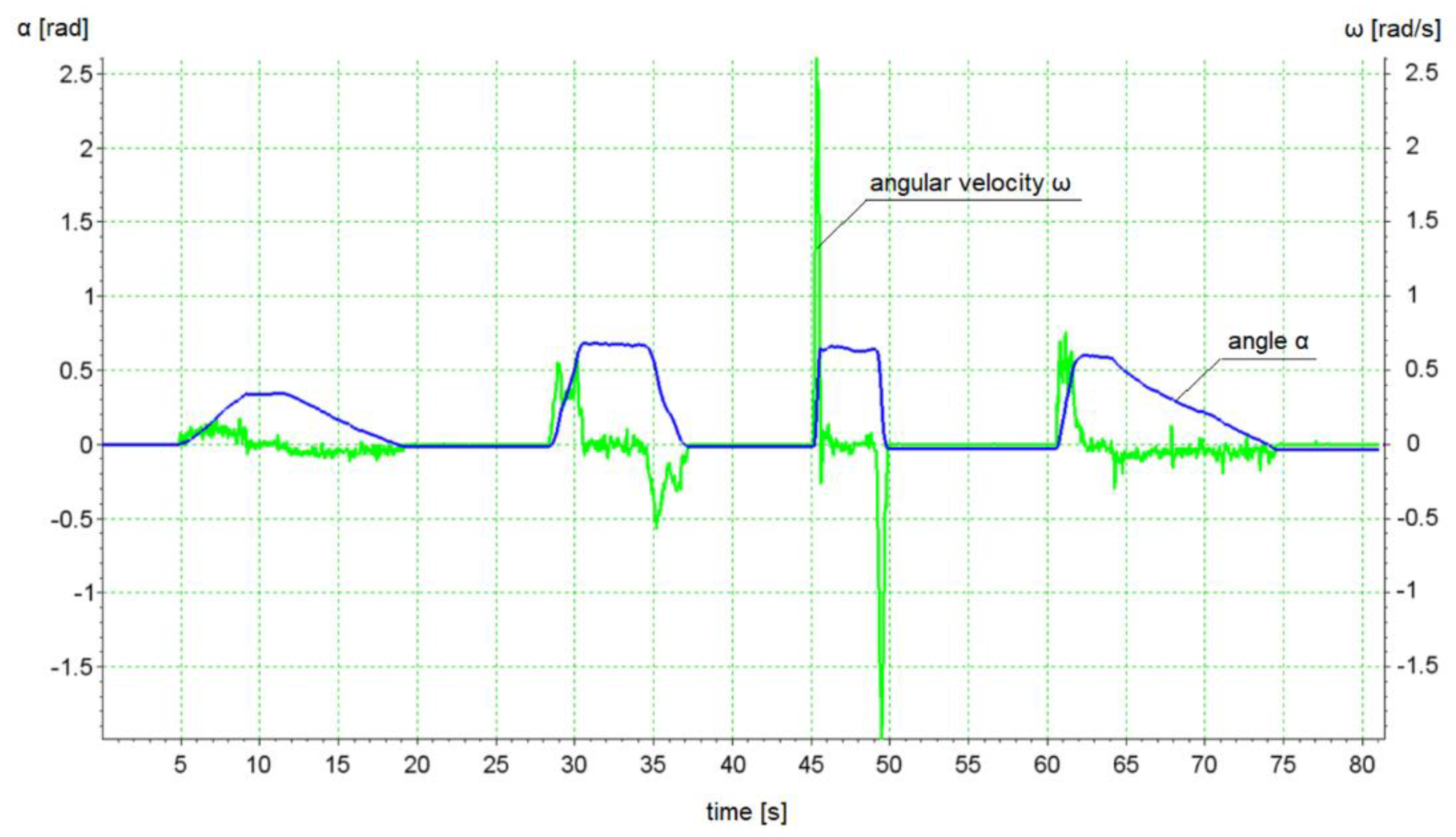
In the research, a series of tests were performed to check the repeatability of angle measurements. In the case in question, a triaxial MEMS gyroscope was used. The tilt angle of the platform was measured and the obtained calculation results were compared. The tests showed very high convergence of single angular measurement. However, at the same time, rapid accumulation of measurement uncertainty due to the overlapping of measurement errors has been reported. The readout difference of 2 degrees was recorded after only four tilts of the scaling device (tests were made with different rotational speeds). The test results present
Figure 2. The measured difference was equivalent to a 52 mm cant. This means that the error is 10 times greater than the permissible value according to the previously mentioned standards [
26,
27,
28].
Based on the results of above tests as well as previous authors’ experience, it was assumed to desist the gyroscopic measurement due to the probable accumulation of errors during measurement (centrifugal accelerations and vehicle vibration). The possibilities for using accelerometric measurements were then focused on. Such a measurement will be regarded in further considerations as the addition of redundant information which allow the verification of indications of other devices to increase the measurement reliability.
2.3. Theoretical Assumptions for Cant Calculation
The difference between the rail heights is reflected in the angle by which a moving vehicle turns. The relationship between cant and the vehicle tilt angle is described by the following Formula:
where:
- D
– Cant [mm],
- e
– Centreline spacing of the rails [mm],
- α
– Vehicle’s angle of inclination in relation to the plane [rad].
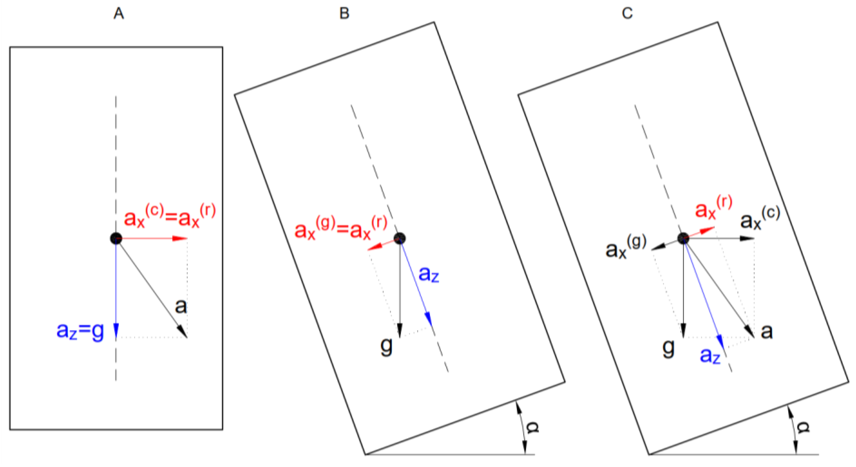
In a vehicle that is stationary (or is moving along a perfectly straight track in the horizontal plane), the cant can be measured using the change in the standard gravity component value measured transversely to the car (
Figure 3b).
where:
– Acceleration transverse to the car body [m/s2],
- g
– Standard gravity [m/s2].
In a moving vehicle, during the movement along a circular curve without cant, an additional transverse acceleration component (centrifugal) will appear, as shown in
Figure 3a. Where a vehicle is regarded as a point particle, the relationship between the velocity, curve radius, and the centrifugal acceleration is as follows:
where:
– Centrifugal acceleration [m/s2],
- v
– Vehicle’s linear velocity [m/s],
- R
– Curve radius [m].
When a vehicle is moving along a curve with a cant, the above-mentioned states are combined (
Figure 3c). The measured acceleration transverse to the car body will depend on the components derived from the gravity and centrifugal acceleration:
Given the small values of the angle
(in practice not exceeding 6 degrees), it can be assumed approximately that its cosine is equal to 1. Such an assumption simplifies the calculation process. Basing on Formulas 4–7, the cant can be calculated using the following relationship:
where:
In the presented relationship, the unknowns include the transverse acceleration, the vehicle movement velocity, and the curve radius (in general—curvature). The simultaneous determination of these three values requires the application of a complex measurement technique.
In order to solve the defined problem for existing tracks, the authors developed an algorithm which uses signals from GNSS and INS measurements. The analytical form of the algorithm and its operation will be illustrated in next sections.
2.4. Calculation of Ccorrections—Algorithm
The initial step in determining the cant is the rough (automatic) analyses of the obtained measurement signal. Based on the GNSS signal analysis, the track curvature at any given point and the azimuth of the tangent to the track axis at that place are determined.
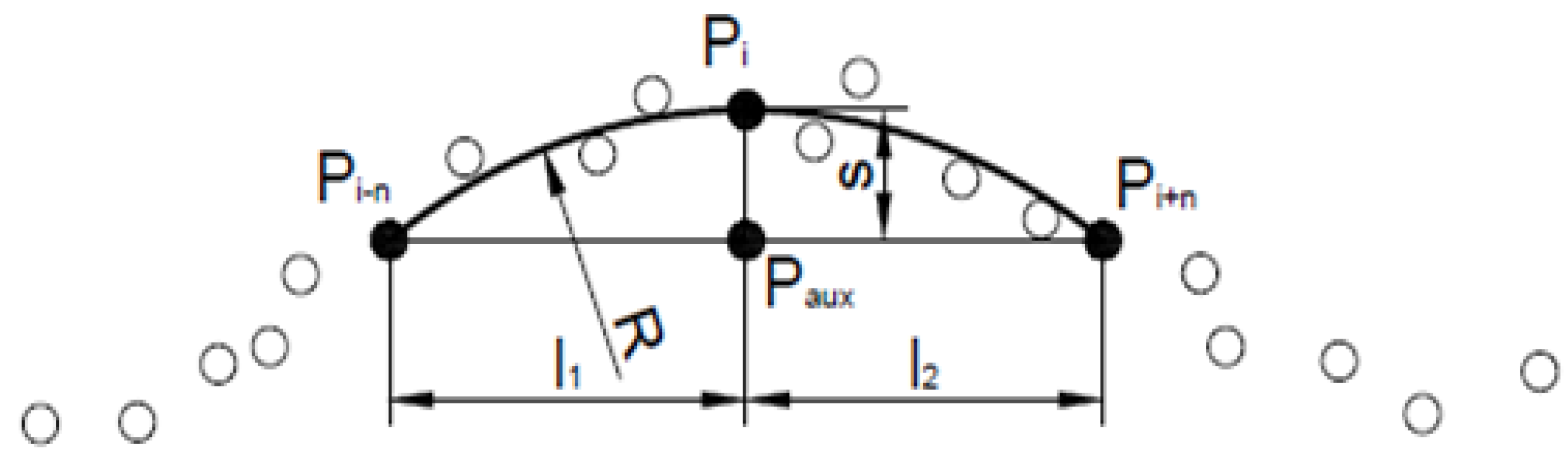
The track curvature radius can be roughly determined based on an analysis of horizontal versines. Since this method is affected by numerous uncertainties, it is regarded exclusively as a preliminary solution bringing the measured signal closer to the actual track axis shape. To this end, for each of the measured points, a 20 m long virtual chord is introduced (10 m on each side of the point) and the value of the horizontal versine for this point is calculated (
Figure 4).
Considering that the length of a chord sections
and
may generally be different from each other, the following relationship is used to calculate the arc radius:
where:
- s
– Versine [m],
- l1, l2
– Length of the curve chord part [m].
After expanding of this expression into a Maclaurin series and its conversion to calculate the radius, the corresponding relationship is expressed by the following Formula:
where:
- Xp
– The northern coordinate in the Cartesian coordinate system [m],
- Yp
– The eastern coordinate in the Cartesian coordinate system [m],
- i
– Measurement index,
- n
– Natural number,
- P(aux)
– Auxiliary point.
The first operation to be carried out to calculate the auxiliary point coordinates is to calculate the equation of the straight line passing through the two points that determine the chord and of the straight perpendicular line passing through the point at which the curvature radius is being determined:
The coefficients of the equation of a straight perpendicular line passing through the central point are as follows:
and the auxiliary point coordinates are as follows:
where:
- m
– Straight line inclination,
- b
– Absolute term [m].
Then, for each pair of coordinates measured by the satellite method, the time interval between the previous and the next measurement is determined (with an accuracy of 0.01s). Later on, for this time interval, a mean value of the measured acceleration is measured (the acceleration is measured with a frequency of 100 Hz, therefore there are an average of 10 single acceleration measurements per a pair of coordinates). Since half of the analyzed acceleration signal is then introduced into calculations for the next point, the method in question is identical to the analysis of a signal in a time series using a moving average.
The measuring set’s movement velocity is also determined based on the analysis of distances between the measured points and on the measurement performance time.
The curvature radius, transverse acceleration, and velocity values calculated in this way provide a basis for the calculation of the cant value (according to Formula 8). The next step is the calculation of the value of the necessary shift (correction) of coordinates in the horizontal zone (according to Formula 1) and the shift direction. Given that the coordinates determined by the satellite method are affected by a known uncertainty (determined by the logger), the equation of the straight line perpendicular to the shift direction was calculated using a weighted regression of a specific number of coordinates (determined by the satellite method) found in the vicinity of this point.
where:
- χ2
– Random variable chi-squared distribution [m2],
- j
– Measurement index.
The corrected coordinates are calculated using the following relationships:
2.5. Advanced Analysis of the Geometric Layout
The algorithm for the automatic cant calculation presented above is sensitive to the measurement uncertainties. During the analyses, numerous tests involving the filtering of the measurement signal in the wave number domain were carried out. This enabled a reduction of standard errors in the determination of the track axis coordinates associated with the signal oscillation around its actual position.
In order to calculate the design parameters of the track in horizontal plane and cant variability, a theoretical model based on known and common utilizing types of curves needs to be constructed [
31]. For this purpose, SATTRACK program algorithms were used and modified [
12]. Based on the roughly corrected coordinates of the measured track axis, basic geometric parameters are determined by dividing the track into sections of constant and variable curvatures. The analyzed route is then described using parametric equations and its basic characteristic parameters are determined, inter alia:
Straight line azimuths,
Route intersection angles,
Curve radii,
Transition curve lengths,
Model of curvature distribution on the transition curve lengths.
Based on the route described in this way, coordinates of characteristic points are calculated, e.g.,:
It is assumed that on a straight section and on the circular part of the curve, the curvature is constant and has a value of
for the straight section and
on the circular part of the curve. On transition curves, the curvature is variable and described using the following relationship:
For the clothoid, function
takes on the following values:
where:
- κ(l)
– Curvature function,
- g(l)
– Distribution function,
- l
– Distance parameter, along a curve,
- L
– Length of a transition curve.
In order to facilitate calculations, it was assumed that the transition curve arc length is approximately equal to the length of its projection. The distance from the start of the transition curve to the measured point located on its length is calculated based on the following relationship:
The calculations of the shift direction depend on which geometric layout element the measured pair of coordinates is assigned to.
For calculations of the shift direction for a point located on the length of a circular curve, the following Formula is used:
for a point located on the length of a straight section:
and for a point located on the length of a transition curve:
where
—the angle of the tangent to the transition curve arc at a point distant by a certain length from its start. For the clothoid, function
takes on the following values:
where:
- l
– The location (distance from the start) of the point on the transition curve [m],
- g(l)
– Function of variable l, depending on the transition curve type,
- L
– Transition curve length [m],
- TS
– The start of the transition curve (Transition—straight),
- O
– Circle centre.
After performing the calculations, each measured pair of coordinates is assigned additional parameters:
Curvature,
Shift direction,
Velocity,
Acceleration,
Calculated cant value.
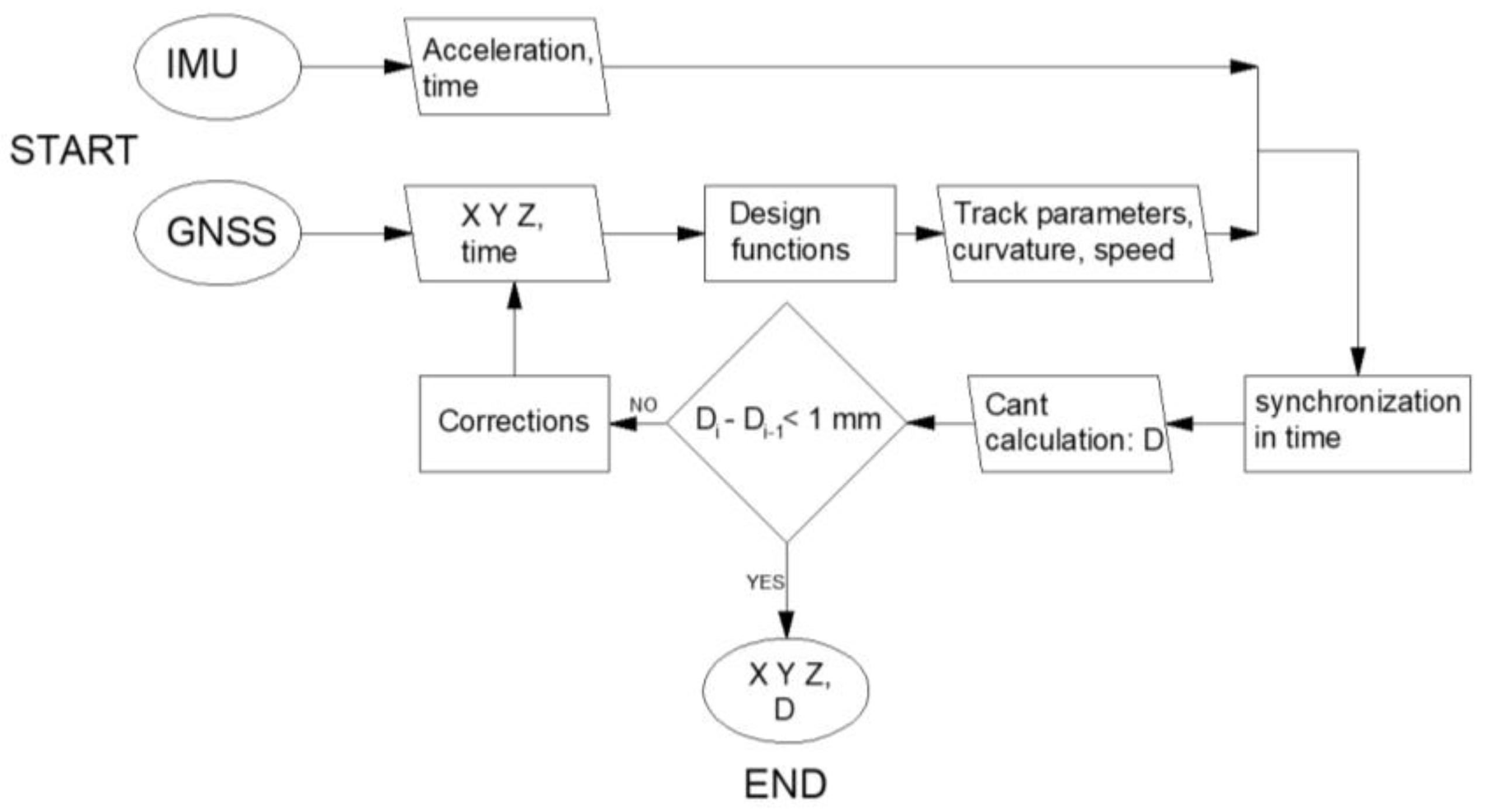
The final step of the analysis is the restoration of the model course of the cant variability and the calculation of corrected track axis coordinates (based on Formulas 19-20). The operation principle of the calculation algorithm is presented in the diagram in
Figure 5.
3. Results
In order to verify the presented methodology for the correction of coordinates obtained by the MSM method, a series of both satellite and accelerometric measurements were carried out as well as additional reference measurements using a manual track gauge. A tram line fragment consisting of a curve with a cant and the adjoining straight sections was selected.
For the measurement of accelerations, an MPU-6500 triaxial MEMS accelerometer was used. This accelerometer is comprised of microscopic movable elements which deflect under the action of acceleration in the corresponding direction. The device determines the change in the system’s capacitance and, based on that, calculates the deflection of the element and the associated acceleration on a particular axis. The rotation of the device casing results in a change in the direction of standard gravity’s action on the accelerometer and, consequently, enables the calculation of the rotation angle.
The cant on the curve and on the adjoining straight sections was then measured using a manual track gauge. On the straight sections, the measurements were taken every 10 m. The restored lengths of the curve and ramps are shown in
Figure 6. The measurement is marked in blue while the identified linear estimation of the cant variability is in green. It was found that the surveyed layout comprised of two cant transitions and a section with a constant cant value. The cant transitions were not located on transition curves that were not detected on the surveyed geometric layout.
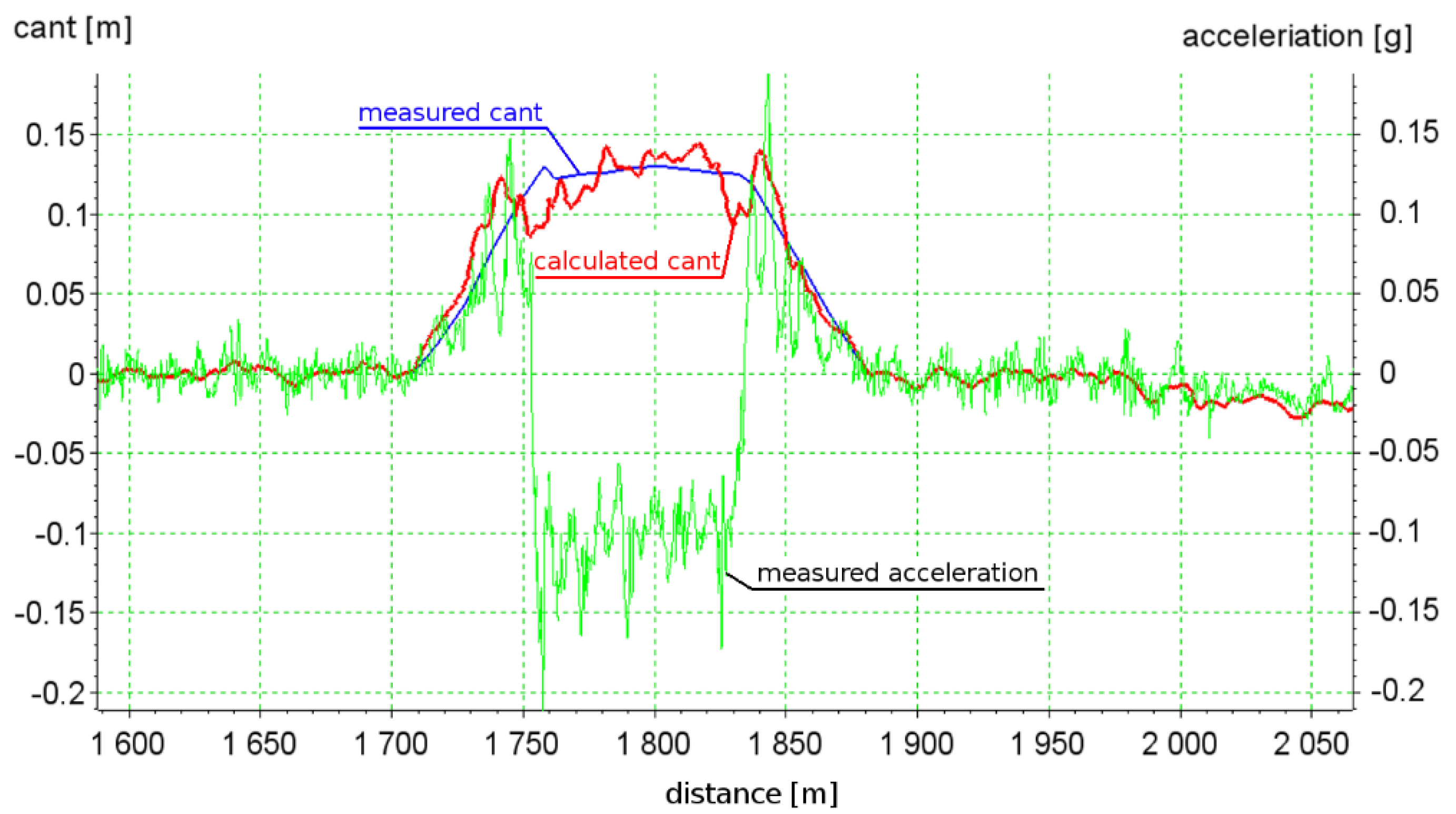
An automatic measurement of cant was then taken using the algorithm described above. Measurements were carried out at various velocities of the measuring vehicle. On a properly maintained track, a change in the vehicle velocity had no significant effect on the results of the conducted analyses. An analysis result for the highest of the recorded velocities, i.e., 60 km/h, is shown. A graph of the variability of the recorded acceleration and the restored cant is shown in
Figure 7. On straight sections, the estimated cant oscillates around 0, and on the cant transitions (located on the straight sections of the track) an evident increase occurs in the acceleration as well in the calculated cant. At the connection between the straight line and the curve (at the point of tangency which is also a point of the super-elevation ramp end), a rapid change in the direction of acceleration action occurred. After passing this point, the calculated cant value remained at a relatively constant level. An opposite situation occurred at the transition from the curve into the straight line and on the second cant transition.
It can be noted that both the restored value of the cant on the curve and the cant variability on the length corresponds to the values measured using the manual track gauge. A mean value of the cant on the circular part of the curve, measured based on the measurement of accelerations, differs by 2 mm (for a velocity of 53 km/h) from the value measured using the track gauge. The oscillation of the restored cant results from the GNSS measurement errors and the induced vibrations of the measuring vehicle itself.
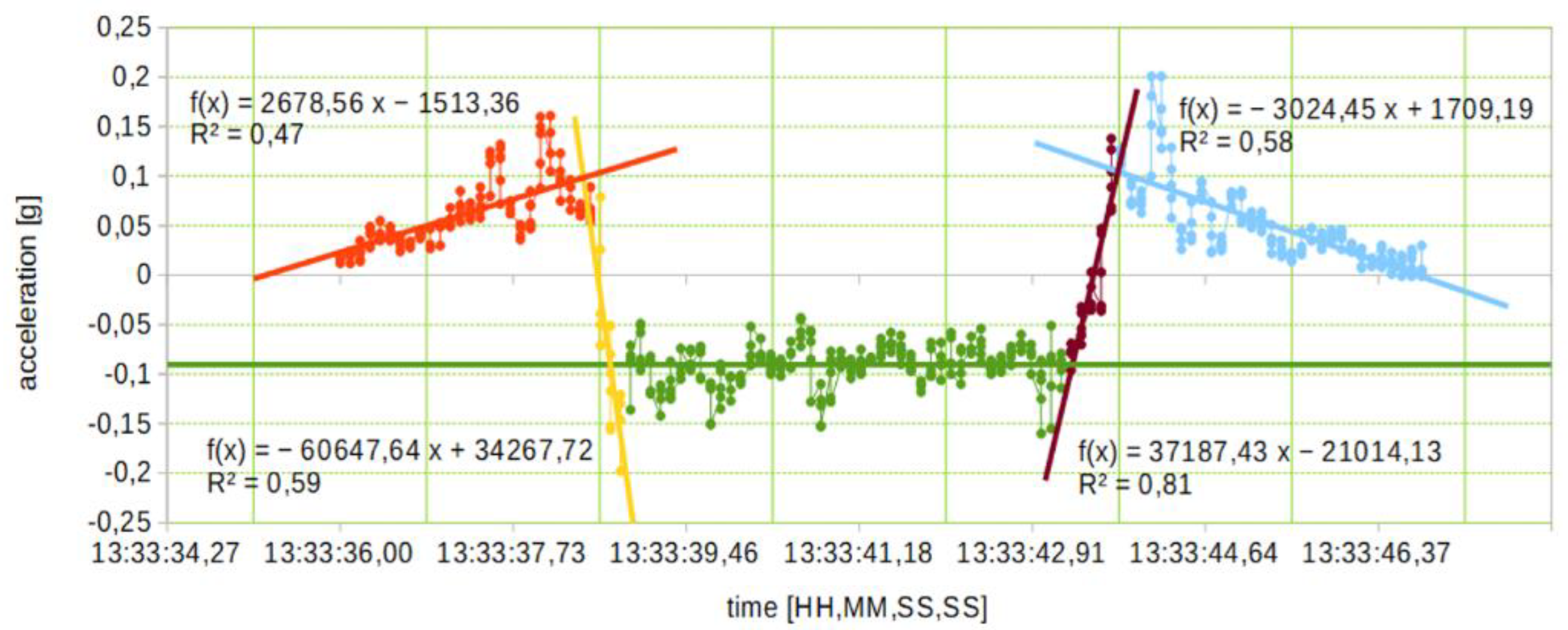
The acceleration variability during a passage of the measuring car was then calculated. In order to better illustrate the possibilities offered by the presented methodology, a passage at a velocity of 60 km/h was selected.
Figure 8 shows a graph of acceleration variability at the time of running along the curve (only the section between the start of the first cant transitions and the end of the second one is shown).
It is evident that this track segment can be divided into five sections characterized by different acceleration variability parameters:
Red and blue color—the cant transition located on a straight section. In a model fashion, it is characterized by a constant increase in acceleration, while in reality, given the tram car design, strong oscillations occur at the end of the cant transition,
Yellow and purple color—a rapid change in acceleration associated with the change in curvature at the point, determined by the length of the car’s rigid base,
Green color—a circular part of the curve characterized by constant curvature and cant. In a model fashion, acceleration should have a constant value as well. However, the vibrations induced on the cant transition are clearly detected.
Based on the acceleration value regression in the indicated intervals and the analysis of the restored cant variability, a model of cant on the curve’s length was constructed. A graph of identified cant variability corresponds to that measured using a track gauge with a relatively high accuracy. Parameters of the restored cant variability are shown in
Table 1.
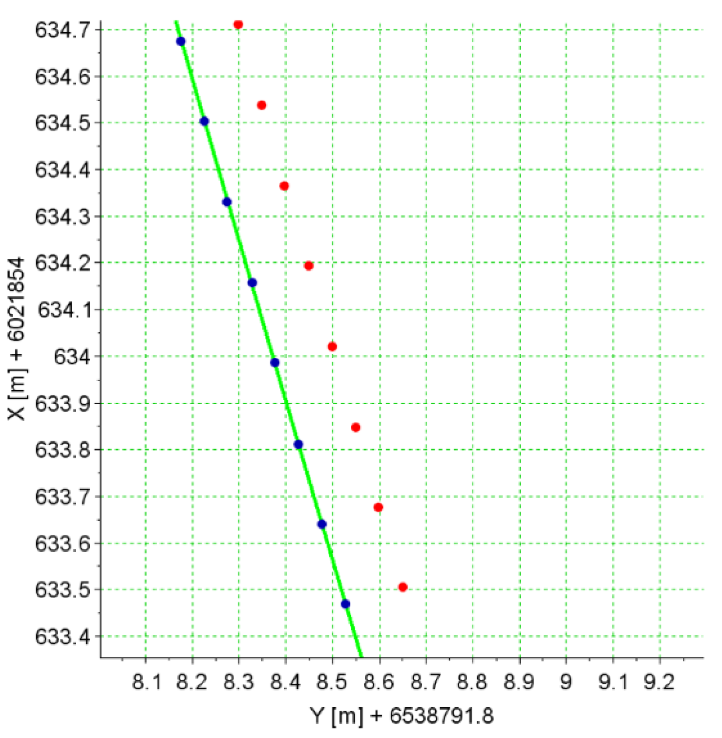
The last step of the analysis was to introduce corrections to the measured track axis coordinates.
Figure 9 shows a fragment of the measured curve. The measured coordinates that were characterized by a constant shift in relation to the model location of the track axis (green line) due to the measuring vehicle’s tilt are marked in red. The coordinates corrected by the value of
are marked in blue. As can be seen, they coincide with the expected location of the track axis.
4. Discussion
In this section, the effects of the algorithm operation have been presented and discussed. In order to assess the effectiveness of the analysis, differences between identified layout and the reference one from the measurement were analyzed.
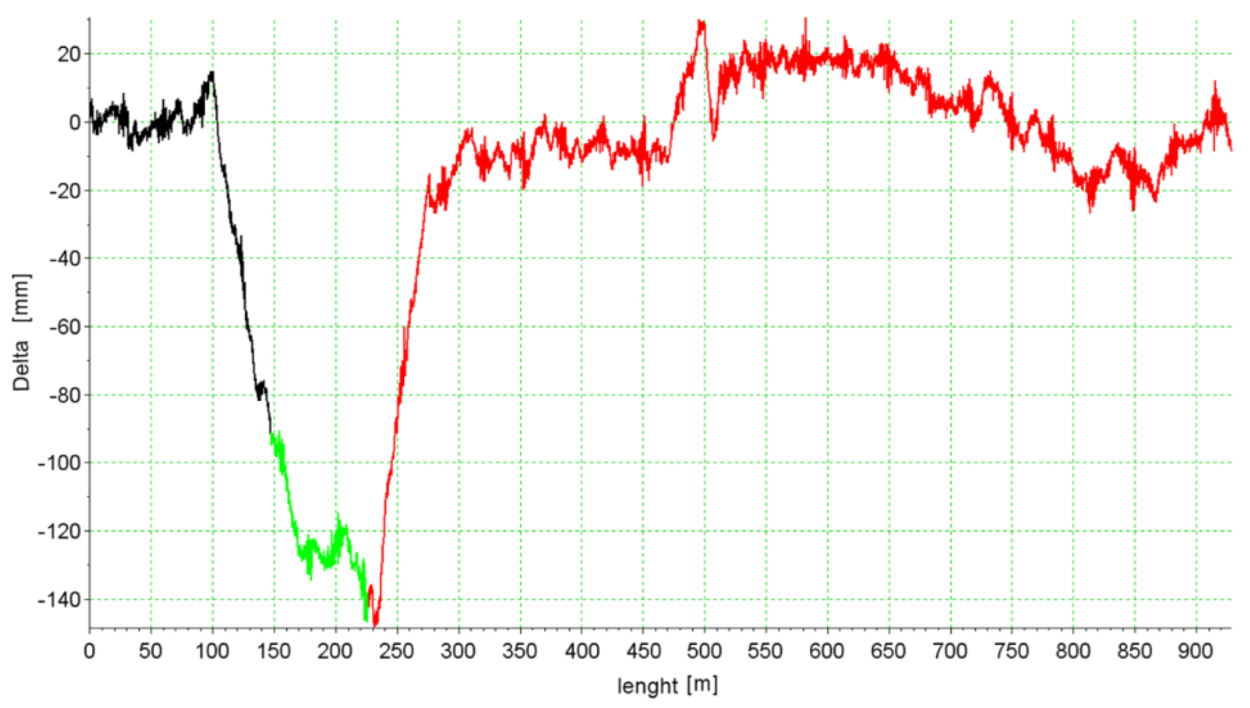
Figure 10 shows effect of track layout estimation. The signal clearly shows the presence of super-elevation ramps which are located on straight sections (an evident linear increase in delta differences) and of cant with a constant value on the curve.
Knowing that this layout has no transition curves, it becomes obvious that this about 130 mm shift in the central part of layout should be corrected.
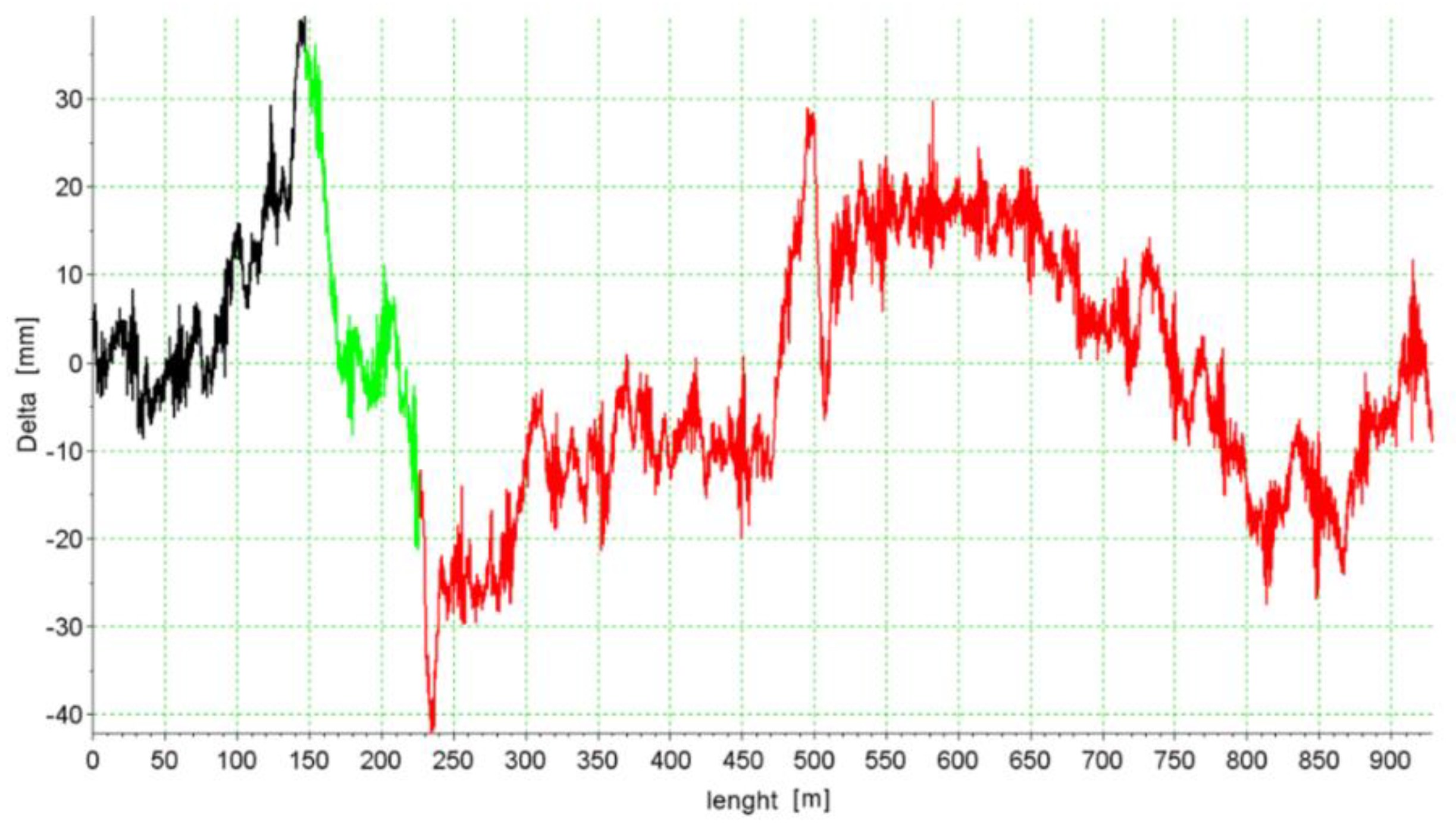
Figure 11 shows the effect of correction. An improvement in layout estimation can be noticed. Deviations between estimation and measured positions for the corrected coordinates are relatively evenly distributed on the length of the section (straight sections are marked in black and red, while the circular curve is marked in green).
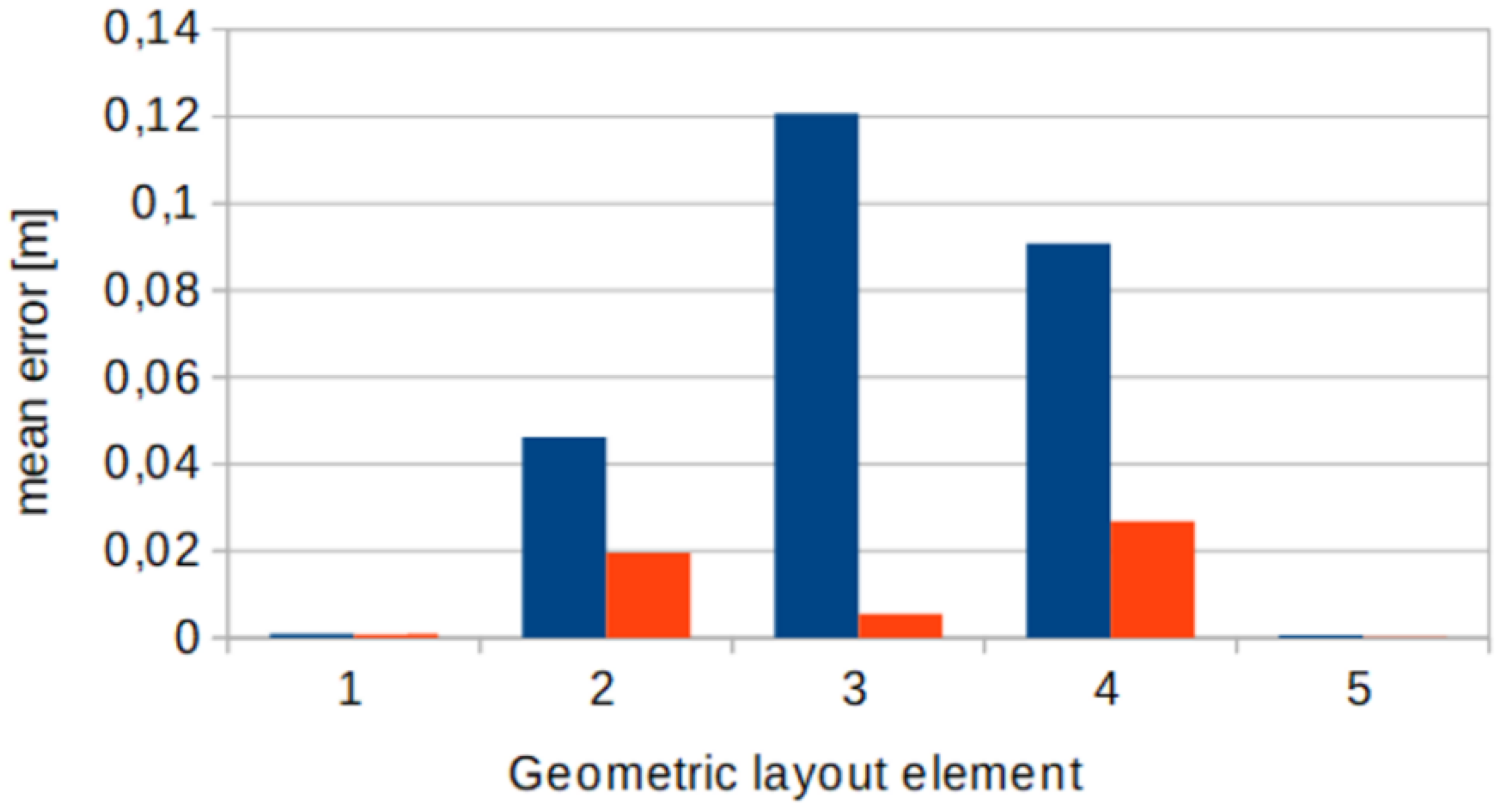
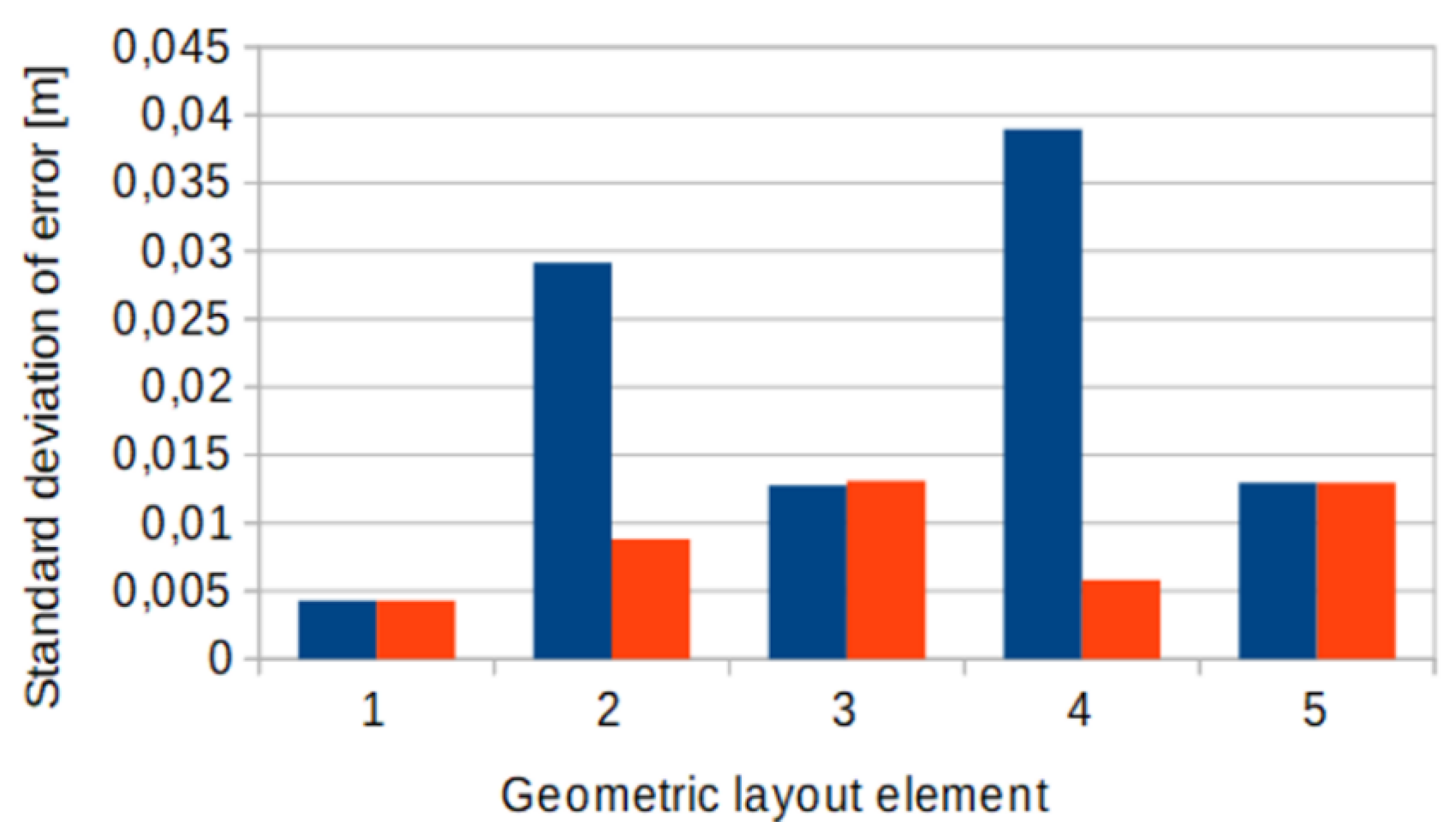
Apart from the clear decrease in the uncertainty of the route course estimation that is visible while comparing also
Figure 12 and
Figure 13, the mean values of the differences and their standard deviations also clearly decreased. However, a shift of the mean value on the sections with cant in relation to the sections with no cant can still be seen. Relatively higher values may be correlated with deformations of existing track axis along the curve or can be the effect of measurement quality.
5. Conclusions
The Mobile Satellite Measurement method enables the efficient and effective reconstruction of the railway and tram tracks geometry. Its supplementation by including measurements concerning the cant, presented in the paper, enable a further enhancement of measurement reliability and accuracy.
As has been demonstrated, it is possible to measure cant using accelerometry. Thanks to the use of standard gravity variability, this is a certain method as the obtained results are not determined by the previous location of the device or its indications. For this reason, no measurement result drift occurs and there is no need to perform precision device calibrations (a measurement can be started on a track with any given cant or twist).
In this particular case, even the use of standard, easily available measuring devices allowed obtaining satisfactory results. The use of a more complex measuring system would have yielded results of a probably significantly higher quality. In further research, it will be advisable to create a common logger for satellite and accelerometric measurements in order to avoid the need for signal synchronization in the time domain which, by assumption, introduces an additional uncertainty due to measuring device clock errors.
Author Contributions
Conceptualization, W.K., C.S., J.S., P.C.; methodology, W.K., C.S., J.S., P.C.; software, J.S., P.C.; validation, J.S., P.C.; formal analysis, J.S., P.C.; investigation, C.S., W.K., J.S.; resources, C.S., J.S.; data curation, C.S., J.S., P.C.; writing—original draft preparation, J.S., P.C.; visualization, J.S., P.C.; supervision, W.K., C.S.
Funding
This research received no external funding.
Acknowledgments
The authors would like to thank the Municipal Transport Company GAiT (Gdansk, Poland) for their support in the field research.
Conflicts of Interest
The authors declare no conflict of interest.
References
- Parkinson, B.W. Global Positioning System: Theory and Applications; American Institute of Aeronautics and Astronautics: Reston, VA, USA, 1996; Volume 1. [Google Scholar]
- Lichtberger, B. State of Chord Measurement Using EM-SAT or GPS. El/Der Eisenbahningenieur 1995, 46, 560-ff. [Google Scholar]
- Szwilski, T.B. Determining rail track movement trajectories and alignment using HADGPS. In Proceedings of the AREMA 2003 Annual Conference, Chicago, IL, USA, 5–8 October 2003. [Google Scholar]
- Gao, Z.; Ge, M.; Li, Y.; Shen, W.; Zhang, H.; Schuh, H. Railway irregularity measuring using Rauch–Tung–Striebel smoothed multi-sensors fusion system: Quad-GNSS PPP, IMU, odometer, and track gauge. GPS Solut. 2018, 22, 36. [Google Scholar] [CrossRef]
- Groves, P.D. Principles of GNSS, Inertial, and Multisensor Integrated Navigation Systems, 2nd ed.; Artech House: Norwood, MA, USA, 2013. [Google Scholar]
- Specht, C.; Weintrit, A.; Specht, M. A History of Maritime Radio-Navigation Positioning Systems Used in Poland. J. Navig. 2016, 69, 468–480. [Google Scholar] [CrossRef]
- Sitnik, E.; Oszczak, B.; Specht, C. Availability Characteristics Determination of FKP and VRS Techniques of ASG-EUPOS System. In Proceedings of the 14th International Multidisciplinary Scientific GeoConference SGEM 2014, Albena, Bulgaria, 17–21 June 2014; pp. 97–104. [Google Scholar]
- Specht, C.; Specht, M.; Dabrowski, P. Comparative Analysis of Active Geodetic Networks in Poland. In Proceedings of the 17th International Multidisciplinary Scientific GeoConference SGEM 2017, Vienna, Austria, 27 June–6 July 2017; Volume 17, pp. 163–176. [Google Scholar]
- Chen, Q.; Niu, X.; Zhang, Q.; Cheng, Y. Railway track irregularity measuring by GNSS/INS integration. Navigation 2015, 62, 83–93. [Google Scholar] [CrossRef]
- Specht, C.; Nowak, A.; Koc, W.; Jurkowska, A. Application of the Polish Active Geodetic Network for Railway Track Determination. In Transport Systems and Processes. Marine Navigation and Safety of Sea Transportation; CRC Press—Taylor & Francis Group: London, UK, 2011; pp. 77–81. [Google Scholar]
- Specht, C.; Koc, W.; Smolarek, L.; Grządziela, A.; Szmagliński, J.; Specht, M. Diagnostics of the tram track shape with the use of the Global Positioning Satellite Systems (GPS/Glonass) measurements with a 20 Hz frequency sampling. J. Vibroeng. 2014, 16, 3076–3085. [Google Scholar]
- Specht, C.; Koc, W.; Chrostowski, P.; Szmagliński, J. The analysis of tram tracks geometrical layout based on Mobile Satellite Measurements. Urban Rail Transit 2017, 3, 214–226. [Google Scholar] [CrossRef]
- Specht, C.; Koc, W.; Szmagliński, J.; Gajdzica, P.; Specht, M. GNSS inventory of historic narrowgauge railway line in Koszalin under extremely unfavorable measurements conditions from the point of view of satellite signals availability. In Proceedings of the 1st International Conference on Innovative Research and Maritime Applications IRMAST 2015, Gdansk, Poland, 23–24 April 2015; pp. 3–8. [Google Scholar]
- Specht, C.; Koc, W.; Chrostowski, P. Computer-Aided Evaluation of the Railway Track Geometry on the Basis of Satellite Measurements. Open Eng. 2016, 6, 125–135. [Google Scholar] [CrossRef]
- Koc, W.; Specht, C.; Chrostowski, P.; Palikowska, K. The accuracy assessment of determining the axis of railway track basing on the satellite surveying. Arch. Transp. 2012, 24, 307–320. [Google Scholar]
- Specht, C.; Koc, W.; Chrostowski, P.; Szmagliński, J. Accuracy assessment of mobile satellite measurements in relation to the geometrical layout of rail tracks. Metrol. Meas. Syst. 2019, 26, 309–321. [Google Scholar]
- Specht, C.; Koc, W.; Chrostowski, P.; Szmagliński, J.; Skóra, M.; Dąbrowski, P.; Specht, M.; Dera, M. Mobile Satellite Measurements on the Pomeranian Metropolitan Railway. Transp. Overv. 2016, 5, 24–35. [Google Scholar] [CrossRef]
- Leica Geosystems AG. Leica Viva GS16 Data Sheet. Available online: http://leica-geosystems.com/-/media/files/leicageosystems/products/datasheets/leica_viva_gs16_gnss_smart_antenna_ds.ashx?la=en. (accessed on 14 October 2019).
- Koc, W.; Specht, C. Selected problems of determining the course of railway routes by use of GPS network solution. Arch. Transp. 2011, 23, 303–320. [Google Scholar] [CrossRef]
- Comite Europeen de Normalisation. European Standard EN 13803-1, Railway applications—Track—Track alignment design parameters—Track gauges 1435 mm and wider—Part 1: Plain line; Comite Europeen de Normalisation: Brussels, Belgium, 2010. [Google Scholar]
- Koc, W. The analytical design method of railway route’s main directions intersection area. Open Eng. 2016, 6. [Google Scholar] [CrossRef]
- Pfister, F.; Reitze, C. The motion equations of rotors, gyrostats and gyrodesics: Application to powertrain-vehicle mechanical systems. Arch. Appl. Mech. 2009, 79, 81–96. [Google Scholar] [CrossRef]
- Godha, S.; Cannon, E. Integration of DGPS with a Low Cost MEMS—Based Inertial Measurement Unit (IMU) for Land Vehicle Navigation Application. In Proceedings of the 18th International Technical Meeting of the Satellite Division of The Institute of Navigation (ION GNSS 2005), Long Beach, CA, USA, 13–16 September 2005; pp. 333–345. [Google Scholar]
- Fong, W.T.; Ong, S.K.; Nee, A.Y.C. Methods for in-field user calibration of an inertial measurement unit without external equipment. Meas. Sci. Technol. 2008, 19, 085202. [Google Scholar] [CrossRef]
- Syed, Z.F.; Aggarwal, P.; Goodall, C.; Niu, X.; El-Sheimy, N. A new multi-position calibration method for MEMS inertial navigation systems. Meas. Sci. Technol. 2007, 18, 1897–1907. [Google Scholar] [CrossRef]
- Comite Europeen de Normalisation. EN 13848-1:2003+A1: 2008 Railway Applications—Track. Track Geometry Quality—Characterisation of Track Geometry; Comite Europeen de Normalisation: Brussels, Belgium, 2008. [Google Scholar]
- Comite Europeen de Normalisation. EN 13848-2: 2006 Railway Applications—Track. Track Geometry Quality—Measuring Systems—Track Recording Vehicles; Comite Europeen de Normalisation: Brussels, Belgium, 2006. [Google Scholar]
- Comite Europeen de Normalisation. EN 13848-3: 2009 Railway Applications—Track. Track Geometry Quality—Measuring Systems—Track Construction and Maintenance Machines; Comite Europeen de Normalisation: Brussels, Belgium, 2009. [Google Scholar]
- Norouzpour-Shirazi, A.; Serrano, D.E.; Zaman, M.F.; Casinovi, G.; Ayazi, F. A dual-mode gyroscope architecture with in-run mode-matching capability and inherent bias cancellation. In Proceedings of the 18th International Conference Solid-State Sens. Actuators Microsyst. (TRANSDUCERS), Anchorage, AK, USA, 21–25 June 2015; pp. 23–26. [Google Scholar]
- Prikhodko, I.P. In-run bias self-calibration for low-cost MEMS vibratory gyroscopes. In Proceedings of the 2014 IEEE/ION Position, Location and Navigation Symposium-PLANS, Monterey, CA, USA, 5–8 May 2014; pp. 515–518. [Google Scholar]
- Koc, W.; Chrostowski, P. Computer-aided design of railroad horizontal arc areas in adapting to satellite measurements. J. Transp. Eng. 2014, 140, 04013017. [Google Scholar] [CrossRef]
Figure 1.
Cross-section of measured track with a cant: e—distance between rails axes; D—cant; α—cant angle.
Figure 1.
Cross-section of measured track with a cant: e—distance between rails axes; D—cant; α—cant angle.
Figure 2.
A graph of the repeatability test of the angle measurement using a gyroscope.
Figure 2.
A graph of the repeatability test of the angle measurement using a gyroscope.
Figure 3.
The distribution of acceleration in different movement patterns. (a) a case of movement along a circular curve without a cant, (b) a case of movement along a tangent section with a cant, (c) a case of movement along a circular curve with a cant.
Figure 3.
The distribution of acceleration in different movement patterns. (a) a case of movement along a circular curve without a cant, (b) a case of movement along a tangent section with a cant, (c) a case of movement along a circular curve with a cant.
Figure 4.
A diagram of track curvature calculation using satellite measurements.
Figure 4.
A diagram of track curvature calculation using satellite measurements.
Figure 5.
Block diagram of the cant calculation and coordinate correction algorithm.
Figure 5.
Block diagram of the cant calculation and coordinate correction algorithm.
Figure 6.
Cant on the curve measured using a manual track gauge.
Figure 6.
Cant on the curve measured using a manual track gauge.
Figure 7.
A graph of the automatically restored cant. The measured acceleration is marked in green, the calculated cant in red, and the measured cant in blue.
Figure 7.
A graph of the automatically restored cant. The measured acceleration is marked in green, the calculated cant in red, and the measured cant in blue.
Figure 8.
A graph of acceleration variability at the time of running along the curve.
Figure 8.
A graph of acceleration variability at the time of running along the curve.
Figure 9.
A comparison of the location of measured and corrected coordinates and the theoretical location of the track axis.
Figure 9.
A comparison of the location of measured and corrected coordinates and the theoretical location of the track axis.
Figure 10.
A graph of the measured track axis deviations in relation to the designed shape.
Figure 10.
A graph of the measured track axis deviations in relation to the designed shape.
Figure 11.
A graph of the measured track axis deviations in relation to the designed shape following the correction of coordinates due to the occurring cant.
Figure 11.
A graph of the measured track axis deviations in relation to the designed shape following the correction of coordinates due to the occurring cant.
Figure 12.
Absolute values of the mean matching error: blue bars—before the correction, red bars—following the correction, 1—straight line 1; 2—super-elevation ramp 1; 3—circular curve; 4—super-elevation ramp 2; 5—straight line 2.
Figure 12.
Absolute values of the mean matching error: blue bars—before the correction, red bars—following the correction, 1—straight line 1; 2—super-elevation ramp 1; 3—circular curve; 4—super-elevation ramp 2; 5—straight line 2.
Figure 13.
Values of the matching error standard deviations: blue bars—before the correction, red bars—following the correction); 1—straight line 1, 2—super-elevation ramp 1; 3—circular curve; 4—super-elevation ramp 2; 5—straight line 2.
Figure 13.
Values of the matching error standard deviations: blue bars—before the correction, red bars—following the correction); 1—straight line 1, 2—super-elevation ramp 1; 3—circular curve; 4—super-elevation ramp 2; 5—straight line 2.
Table 1.
A comparison of the restored cant variability parameters.
Table 1.
A comparison of the restored cant variability parameters.
| Track Section Geometry | Manual Track Gauge | MEMS | Differences |
|---|
| 1st cant transition length | 46.99 m | 46.80 m | 0.19 m | 0.40% |
| 2nd cant transition length | 47.11 m | 44.23 m | 2.88 m | 6.11% |
| Length of the curve with constant cant | 77.54 m | 78.58 m | 1.04 m | 1.34% |
| 1st cant transition steepness | 2.68 mm/m | 2.71 mm/m | 0.03 mm/m | 1.23% |
| 2nd cant transition steepness | 2.67 mm/m | 2.87 mm/m | 0.20 mm/m | 7.33% |
| Mean value of cant | 126.00 mm | 126.48 mm | 0.48 mm | 0.38% |
| Standard deviation of cant | 3.53 mm | 12.20 mm | 8.67 mm | 245.80% |
© 2019 by the authors. Licensee MDPI, Basel, Switzerland. This article is an open access article distributed under the terms and conditions of the Creative Commons Attribution (CC BY) license (http://creativecommons.org/licenses/by/4.0/).


