CFD Simulation of the Wind Field in Jinjiang City Using a Building Data Generalization Method

Abstract

The urban wind environment is an important element of urban microclimates and plays an important role in the quality of the urban environment. The computational fluid dynamics (CFD) simulation method is an important means for urban wind field research. However, CFD simulation has high requirements for computer hardware and software. In this paper, based on geographic information system (GIS) technology, a new building data generalization method was developed to solve the problems of a huge amount of data and calculations in urban-scale CFD wind field simulations. Using Fluent software and high-precision urban building geographic information data with elevation attributes, the method was applied to Jinjiang City, Fujian Province, China. A CFD simulation of the wind field of Jinjiang City was implemented, and detailed, intuitive wind field information was obtained, which were compared with the measured data. The results show that the building data generalization method could effectively improve the efficiency of the city's overall wind field CFD simulation. The simulated wind speed was significantly correlated with the measured data, but it was overestimated. The simulated wind direction was consistent with the measured data of most stations. The simulation results were reasonable and could provide reference for application and subsequent research.

1. Introduction

With the development of the urbanization process, the scale of cities has developed rapidly. Urban construction has changed the natural geomorphologic conditions, and an urban microclimate that differs greatly from the natural climate has been formed [1]. The urban wind environment is an important element of the urban microclimate. Research on the wind field inside the city is an essential basis and premise for evaluating and improving the urban wind environment and plays an important role in improving the urban environment quality [2]. Three kinds of methods have been used in the urban wind field: Field tests, wind tunnel tests and computer numerical simulations. In the early 19th century, Luke Howard conducted an observational study of the urban heat island effect in London, which was the first study of the urban wind environment [3]. Since then, the study of meteorological elements such as temperature and wind in the city through mobile observation technology has been widely adopted in many countries [4,5,6]. However, it is difficult to control meteorological conditions and ground building conditions when using the field test method, and long-term observation of data requires extensive manpower and material resources. Therefore, this method is often used to obtain small amounts of data to compare with other analysis results.

The wind tunnel test is a method of installing an object model in a wind tunnel and studying the air flow and its interaction with the model, and it has been extensively used in recent years [7,8,9]. The wind tunnel test method makes it possible to accurately simulate the flow of wind around a building, but its cost is much higher than the cost of numerical simulation. Moreover, the model ratio should not be too small in order for the conditions of similitude to be satisfied; therefore, this method is not suitable for large-scale wind field simulation.

Computer numerical simulation methods are more cost effective, more efficient and more flexible than the former two methods. Among these methods, the computational fluid dynamics (CFD) method has a powerful calculation and visualization functions and has been widely used in microscale wind environment research in recent years. The CFD method plays an important role in the assessment of the wind environment around the individual buildings [10,11,12], the wind environment of building groups [10,13,14,15,16,17,18,19,20] and the wind environment of the urban block [10,21,22,23,24,25,26,27]. The urban wind environment was evaluated using CFD simulation technology in combination with multiple aspects, including human comfort [28] and pollution spread [29]. The calculation results of the CFD simulation method are intuitive and detailed, and the wind field at any position and any height within the study area can be obtained. Compared with the field test method and the wind tunnel test method, it has advantages. The CFD simulation method is an important technical means for the study of urban wind environments. This method will also be one of the focuses of urban wind field research in the future.

There are a number of studies on the wind field of a single building or a small-area building group, while most of the studies on urban wind fields aim to simulate a typical block in city or generalize the urban building distribution as surface parameters for approximate simulation [30]. One factor contributing to this situation is that the CFD simulation method has high requirements for computer software and hardware resources, which make it difficult to apply CFD to urban-scale wind environment refinement research or to urban overall planning and design. If the traditional CFD simulation process is utilized in the above studies, the consumption of manpower and material resources will be enormous.

In recent years, many scholars have carried out urban-scale wind field simulations based on mesoscale meteorological models such as WRF (Weather Research and Forecasting Model) [31,32,33,34]. However, the resolution of mesoscale meteorological models is up to several hundred meters [31,32,35], which is not sufficiently elaborate for urban planning and engineering. In some studies, a mesoscale model is coupled to a microscale model to provide some ideas for solving this problem [36,37,38,39,40,41]. However, from the perspective of urban overall planning and design, the ability to carry out CFD numerical simulation of the entire urban space as the research object is still of great significance.

In this paper, geographic information system (GIS) technology is used to develop a new method of building data generalization in order to process urban building models to reduce the amount of data and calculations in urban-scale CFD wind field simulations. Using Fluent software, high-precision urban building geographic information data and elevation attribute data, the method was applied to Jinjiang City, Fujian Province, China, a city with an area of approximately 722 square km. Typical wind fields were simulated in which the inflow wind direction is the dominant wind direction and the sub-dominant wind direction, where the inflow wind speed is uniform at each horizontal position of the inflow boundary. The simulation results can provide a reference for urban ventilation planning, but they do not represent the wind conditions at a particular moment. Considering the computational efficiency, temperature change and heat exchange are ignored in this paper. In the following, the study area, data, method and simulation are introduced in Section 2, the results and validation are presented in Section 3, the discussion is presented in Section 4 and finally the conclusion is given in Section 5.

2. Experiments

2.1. Study Area and Data

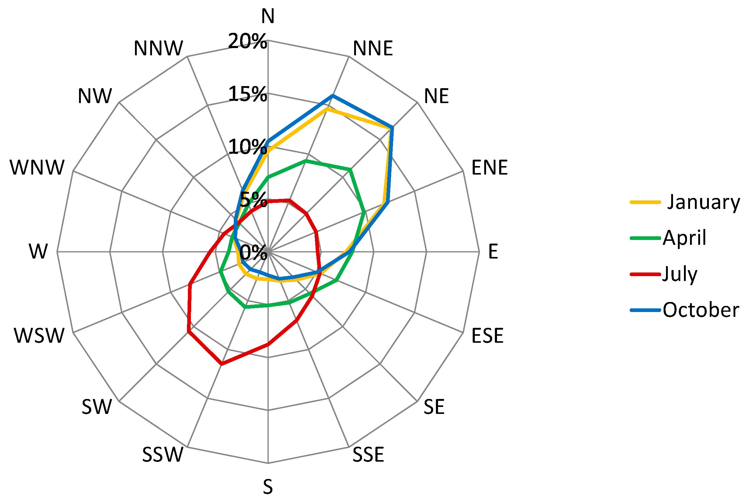
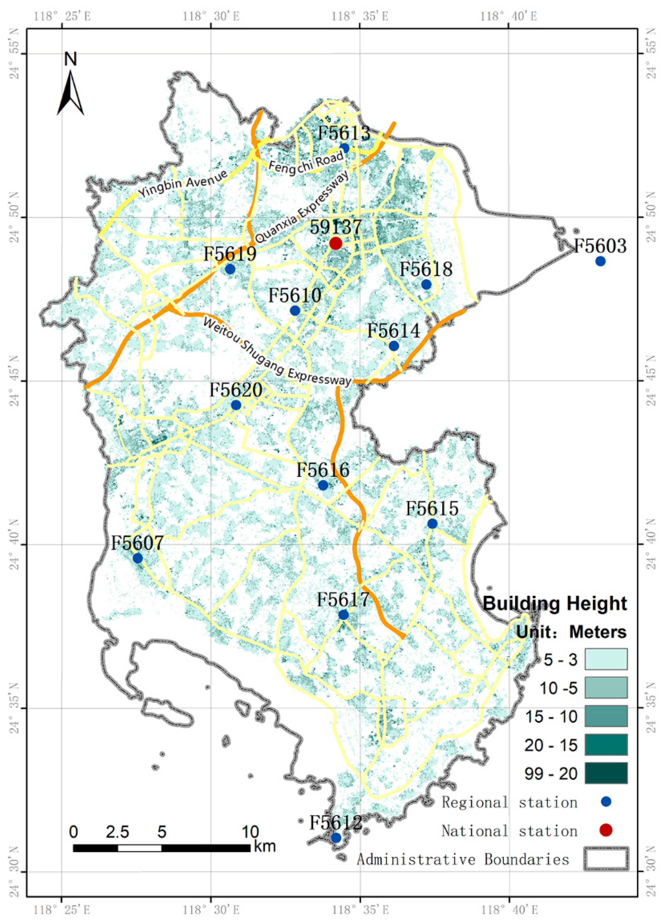
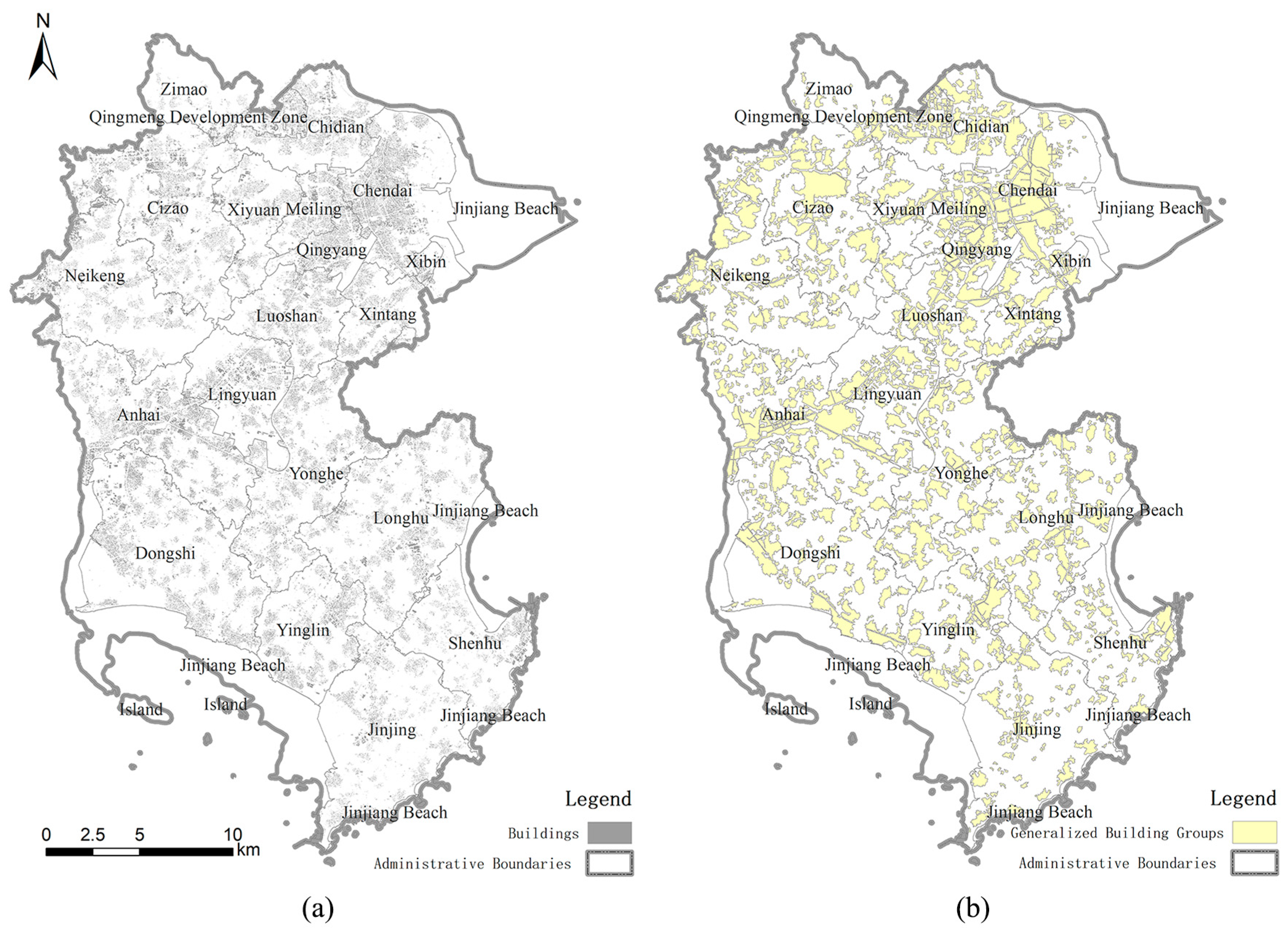
2.1.1. Study Area

The research area Jinjiang City, Fujian Province, is located on the southeast coast of China, at 24°30′44″ N–24°54′21″ N and 118°24′56″ E–118°41′10″ E. The area is in a subtropical marine monsoon climate, and the dominant wind direction has obvious seasonal variation. The area of Jinjiang is approximately 722 square km. The terrain here is quite flat, with three sides facing the sea and the Taiwan Strait in the east, with a coastline of 122 km. Jinjiang City is a booming city that aims to be highly livable. Evaluating Jinjiang City’s urban wind environment and using the evaluation results to assist urban construction planning is of great practical significance to reduce the urban heat island effect and improve the city’s livability.

According to the wind frequency information from national stations and regional automatic stations in Jinjiang from 2010 to 2014, the wind rose diagram for Jinjiang in January, April, July and October was obtained (Figure 1). The typical monsoon climate of Jinjiang has different wind direction frequency distributions in different seasons. The northeast wind prevails in January, April and October, and the southwest wind prevails in July. The wind frequency of the northeast wind in January and October was significantly higher than that in April, indicating that the characteristics of the monsoon in autumn and winter are more noticeable than in spring. In general, the dominant wind direction of Jinjiang is northeast, and the subdominant wind direction is southwest.

Approximately 1.06 million buildings are clustered in Jinjiang City and most of them are distributed along traffic roads. There are highways such as Quanxia Expressway and Weitou Shugang Expressway in Jinjiang. Most roads here are in the northeast-southwest or southeast-northwest direction. High-rise buildings are mainly concentrated in the northeast of the city. Most buildings in Jinjiang are below five floors (15 m), and the highest building is 99 m high. The spatial distribution of buildings in Jinjiang is shown in Figure 2.

2.1.2. Data

Meteorological observation data: Meteorological observations from national stations in Jinjiang and its surrounding areas and some of the regional automatic stations in Jinjiang were used in this paper; mainly hourly wind speed data and wind direction instantaneous value data were used. The data came from the Jinjiang Meteorological Bureau.

Urban building geographic information data: Jinjiang City’s building distribution data and building height data were processed according to a 1:500 topographic map data. The data mainly came from the Jinjiang Bureau of Land and Resources and the Jinjiang Bureau of Housing and Urban-Rural Development.

National fundamental geographic information data of China: The national fundamental geographic information data used in this paper included administrative boundary data and land use data from the National Geomatics Center of China.

2.2. Method and Simulation

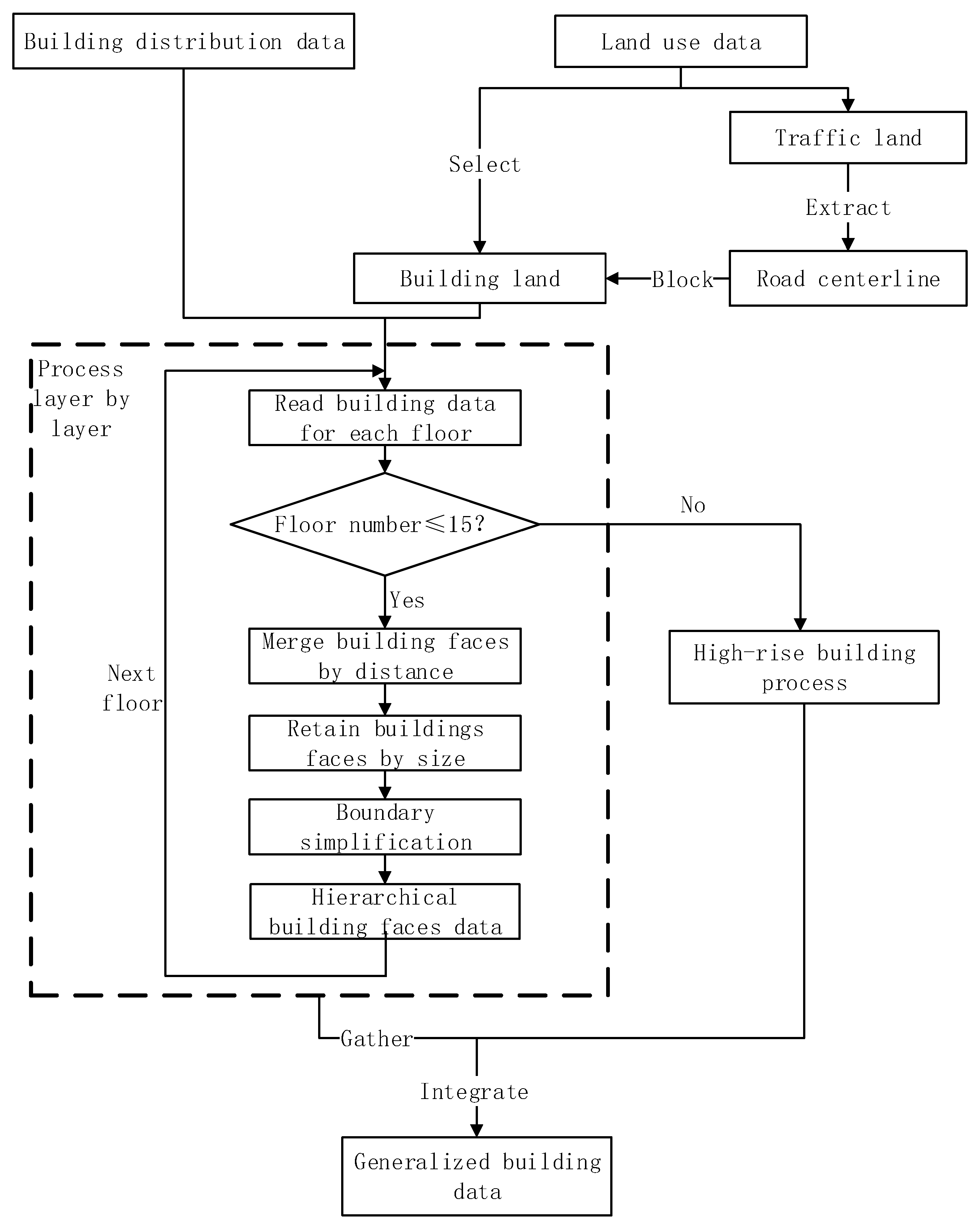
2.2.1. Building Data Generalization Method

Unlike the research area of architectural design environment research or local community planning wind environment research, the study areas of overall urban wind field studies are mostly several hundred square kilometers. Therefore, the CFD wind field simulation on an urban scale faces the challenge of a large simulation area, a large number of urban buildings and complicated architectural model details. If the building data are directly used for modeling in the CFD simulation, the huge amount of geometric data will require excessive manpower, material and time, and the cost will exceed the reasonable range acceptable for practical applications. To simplify the model, to reduce the amount of data and calculation and to make it possible to simulate the wind environment of the whole city within reasonable time and hardware conditions, first, the urban building model would be generalized in this study.

Experiments have found that in the simulation of large-scale urban wind fields, low-rise buildings and buildings with too small an area have little impact on the wind field of the whole city [42]. The gaps in narrow alleys and blocks in the building are extremely low in ventilation and are generally not considered ventilation corridors. Therefore, such overly complex details can be ignored using a generalization method based on GIS technology. Thus, a method of building data generalization is developed to process urban building models to reduce the amount of data and calculations in urban-scale CFD wind field simulations (Figure 3). Using high-precision urban building data in the ArcGIS Shapefile format, a Python script is written to call the toolbox in ArcGIS 10.2 to complete the building data generalization program. The tools in ArcGIS that are called include: Intersect (Analysis), Calculate Areas (Spatial Statistics), Dissolve (Data Management), Buffer (Analysis), Eliminate Polygon Part (Data Management), Multipart to Singlepart (Data Management), Feature Class to Feature Class (Conversion), Polygon to Raster (Conversion), Raster to Polygon (Conversion), Add Field (Data Management), Calculate Field (Data Management), etc.

To generalize building data, a building with a height corresponding to the floor height was first selected into the dataset. The areas where the land use type was road, railway or rural road were selected, the road centerline was extracted and the abovementioned roads with a width greater than a given value were identified. Then, the road shape was simplified using the Douglas-Peucker algorithm [43]. The road area needs to be left blank to prevent street valleys between building groups from being ignored in subsequent operations. Similarly, land parcels where the land use type was cultivated land, forest land, water or unused land were selected; these parcels also need to be left blank. Then, the area that needs to be left blank was erased to obtain the potential building area in the city.

Then, the buildings were intersected with the potential building area in the city. The intersected building layers were organized and the buildings on the same parcel were merged into one geographic element. The minimum distance to be considered between the buildings was set, and buildings with building intervals less than this distance were merged within each parcel. Unnecessary small holes in the merged building model were removed so that the building elements with too small spacing were approximated into an entire building group. There were also a large number of node details and unimportant elements in the building group features. The vector data simplification method was used to simplify the boundary and to remove superfluous details of the building and sharp angles that did not correspond to the actual situation. The small elements with too small areas were also selected and deleted.

Building data of different heights were processed layer by layer to form the building group data of different building heights. The core codes and more description of the technical details for processing each layer were introduced in Appendix A. For non-tall buildings (under 15 floors), each layer of the generalized building data was obtained according to the method described above. Since the degree of influence of buildings of different heights on the urban wind field is different, the area threshold of the reserved building feature was adjusted with the change in the number of floors. For buildings with heights greater than a defined range, only the sidelines were simplified, and the small elements were removed instead of being merged using the generalization method described above. After obtaining the generalized building data of each floor, the data format and height attributes of the layers were sorted, and the data were merged and integrated to obtain generalized building data that could be used for modeling.

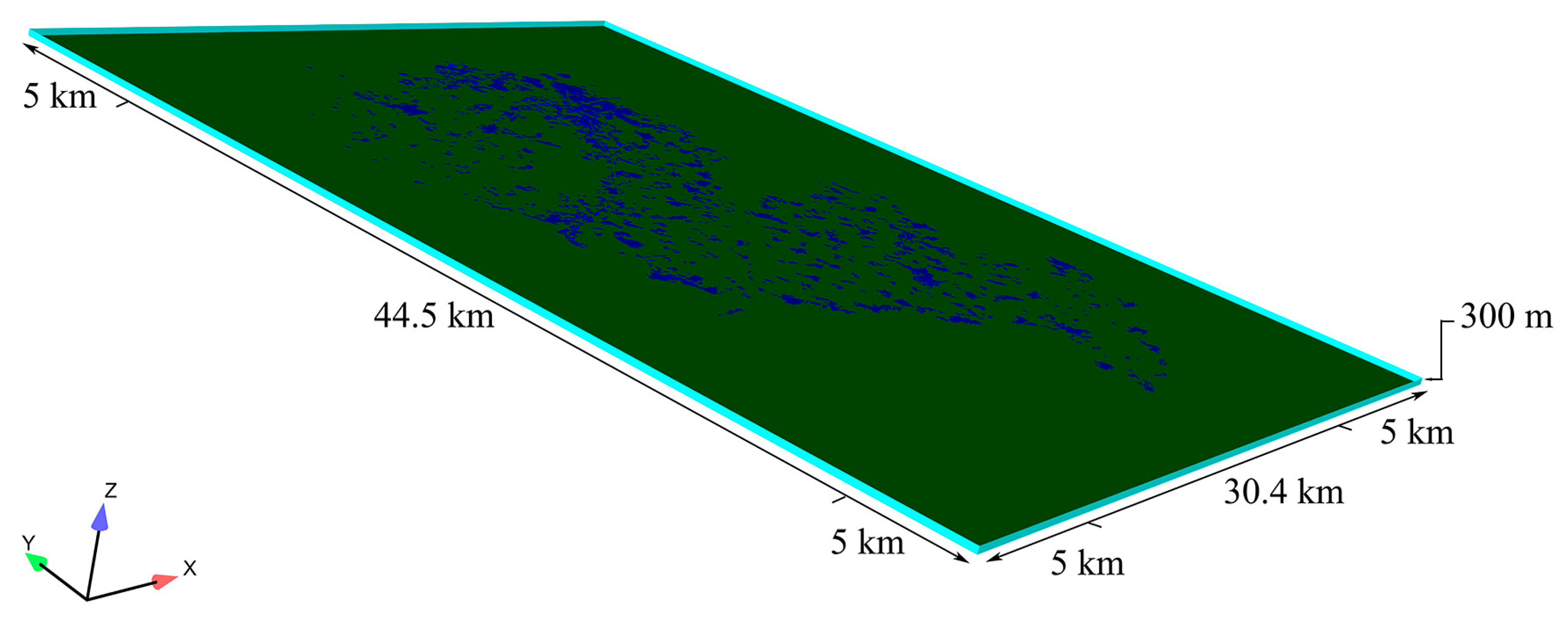
2.2.2. Simulation Models and Parameters

When building the geometric model, a program was written using the C# language and ArcGIS Engine secondary development components to feed GIS data into the CFD preprocessor more accurately and efficiently. The building information in GIS was written into script by the program, and then the script was run directly in the preprocessor GAMBIT to generate a 3D model. A 5000-meter area around the city was expanded to develop the flow field. Including all buildings and surrounding areas, the computational domain was 54.5 km long from north to south and 40.4 km wide from east to west (Figure 4). The height of the domain was 300 m, which was more than three times the height of the tallest building [44]. Buildings with more than two floors were considered when establishing the computational domain.

The boundary of the computational domain in this paper was a complex building model. Therefore, unstructured mesh was selected to divide the fluid domain. The mesh unit was a combination of tetrahedral and pyramidal. In the study, it was expected that the resolution of the area around the building characterized by large changes in wind field characteristics would be under 20 m, which made the resolution and the degree of building model generalization basically the same. For other components, the maximum mesh size could be set larger, so that the mesh was gradually enlarged between the region where the wind field characteristics changed greatly to the small-changed region, so that the number of meshes and the time to generate the mesh were reduced. To test the mesh dependence, we chose different mesh sizes for testing. Due to constraints of computer resources and time, testing over the entire study area was uneconomical and might not be possible due to the high number of meshes. Therefore, we selected a region of about 4 km × 4 km for testing. Three similar simulations, which only differed in the number of meshes (Case 1: 13.25 million, in which the maximum mesh size was 6 m in the building part and 80 m in the ground part; Case 2: 6.63 million, in which the maximum mesh size was 8 m in the building part and 100 m in the ground part and Case 3: 2.10 million, in which the maximum mesh size was 15 m in the building part and 150 m in the ground part) were conducted in this area. 300 random points were taken within 500 m from the buildings, and the difference in wind speed of 10 m height above the ground at these points was observed in the three simulation results (Figure 5). The results show that the wind speeds of Case 1 and Case 2 at random points were very similar, and the difference between them was smaller than their respective with Case 3. The correlation coefficients between Case 1 and 2, and Case 2 and 3 were 0.803 and 0.603, respectively. Although there were some differences between Case 1 and Case 2, the correlation was relatively strong and the data results were also similar. Since the simulation results were intended to provide a reference for urban overall ventilation rather than to study the wind speed at a specific point and time, both mesh parameters in Case 1 and 2 were considered to be usable in the simulation. However, when the maximum mesh size was set as the same as Case 1, the quantity of meshes of the city’s overall simulation was too much, and the resource used will exceed the computer limit. Therefore, the maximum mesh size of the building part and ground part was set to 8 m and 100 m, respectively.

Through experiments, the computational efficiency and the degree of approximation geometry were considered together, and then the mesh parameters of each part of the model were determined as shown in

Table 1. Mesh parameters of each part of the model.

Zone	Maximum Mesh Size
Buildings	8 m
Vertical side face	50 m
Ground	100 m
Top face	100 m

. Most of the meshes’ Y+ was in the recommended range of 30 to 10,000 [45,46,47], and some grids were not within this range due to the limited computer resources and the relatively large computational domain with a complex surface. In order to test the effect of the building data processing method on improving efficiency, considering that Y+ sometimes does not need to be strictly defined in practice, the meshes that were not in the range were retained to obtain the simulation results of the entire city.

The boundary condition types were set in Fluent 15.0 as follows: The vertical boundary (outflow) was set to Pressure-outlet, the vertical boundary (inflow) was set to Velocity-inlet, the top of calculation domain was set to Symmetry and the building surface and ground was set to Wall. The Fluent UDF is written to apply a power law wind profile model to approximate the law of inlet wind speed as a function of altitude [48], which is:

$$\overline{v}\left(z\right)/{\overline{v}}_0={\left(z/z_0\right)}^{\alpha },$$

(1)

where z₀ is the standard reference height, which is taken as 10 m in cities with a roughness height of approximately 100 m, ${\overline{v}}_0$ is the average wind speed at the standard reference height; z represents any height, $\overline{v}\left(z\right)$ represents the average wind speed at any height and α is the ground roughness index, where the rougher the terrain is, the stronger the effect of the surface on the airflow and the greater the α; here α = 0.3 [49].

Based on the actual wind environment in Jinjiang City, two typical wind fields were selected for simulation by analyzing the measured data of the meteorological station. The wind field of the dominant wind direction (NE) and the subdominant wind direction (SW) under the average wind speed of each wind direction was simulated. To simulate the average situation of the urban wind field, the value of the inlet wind speed was set based on the measured data. Using data from the regional automatic weather station on the beach outside Jinjiang City, the average wind speed of the typical wind direction (NE, SW) was calculated, and the wind speed was converted to a height of 10 m according to the power law wind profile model and the elevation of the stations. The data from the meteorological station on the northeastern beach of Jinjiang were used as the inlet wind speed of the dominant wind direction (NE) case. The average data of the weather station on the southwest beach of Jinjiang was used as the inlet wind speed of the subdominant wind direction (SW) case. The inflow wind speed and the direction of typical wind fields are shown in

Table 2. Inflow wind speed and direction of typical wind fields.

Wind Field Case	Wind Direction	Azimuth of Wind Direction (°)	Wind Speed at Standard Reference Height (10 m; m/s)
Dominant wind case	Northeast	45	4.58
Subdominant wind case	Southwest	225	5.77

.

The solution was solved using ANSYS Fluent 15.0 with a finite volume method. The 2-equation k-ε model was selected for turbulence simulation, for it has been widely used in studies on urban wind environment [11,50,51,52,53]. A standard wall function was used, and the solution algorithm was the SIMPLE algorithm. The fluid medium parameter setting used a standard air setting scheme, which was regarded as an incompressible fluid, and the density was set to a constant 1.225 kg/m³ and the viscosity to 1.7894 × 10⁻⁵ kg/m^−s [54]. This paper generated a steady-state low-speed wind field simulation. Due to the complexity of the geometric model, iterative convergence was judged when the continuous residual was stable under 10⁻³ and the calculation result did not change for over 50 iterations.

3. Results and Evaluation

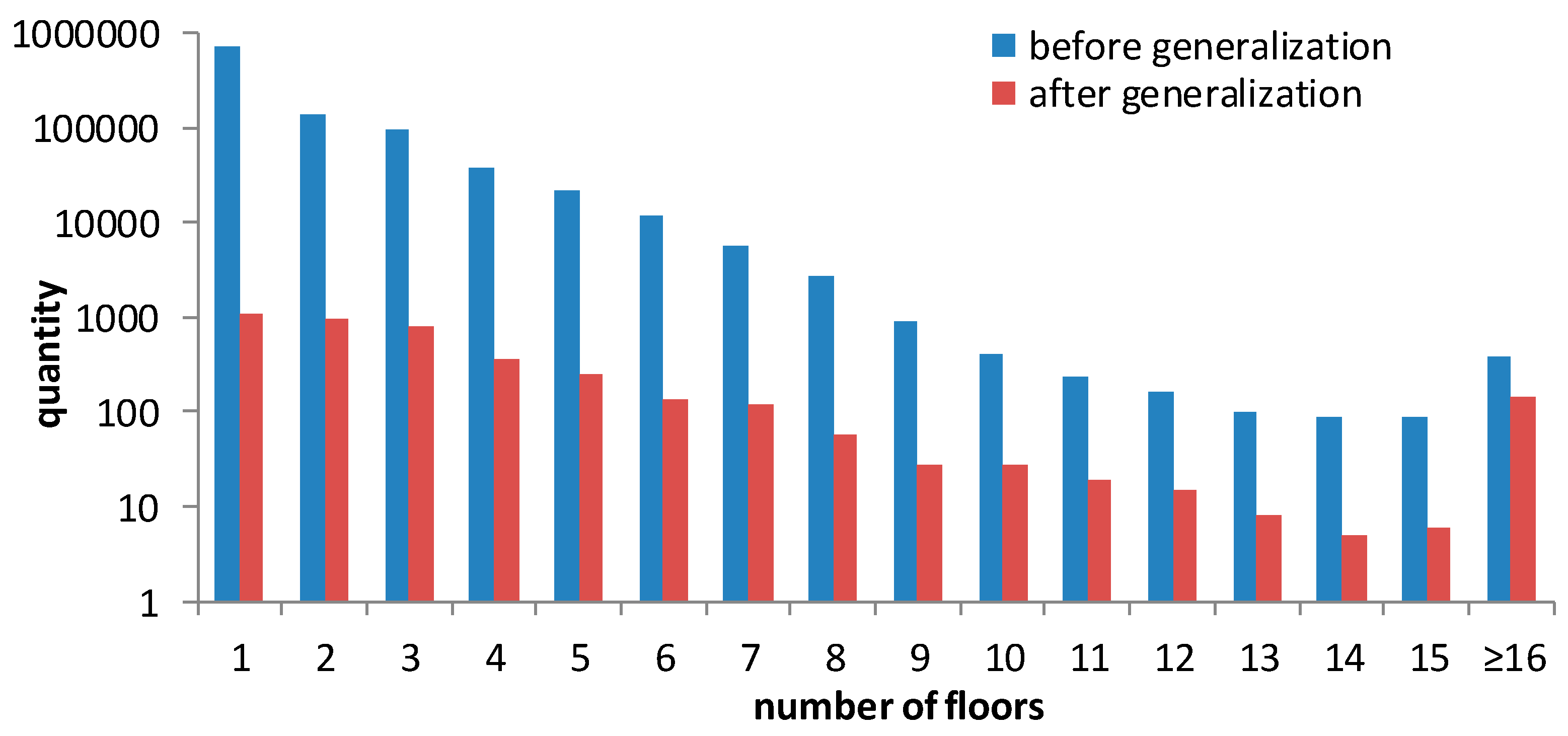
3.1. Building Data Generalization Results

In contrast to the original building map, the densely populated buildings were integrated into building groups, and some low-rise, scattered buildings were ignored. After generalization, a number of building elements at a close distance were merged into one whole building group, but the macroscopic distribution characteristics, such as the shape and orientation of the building group, remained unchanged. The original appearance of large-scale or high-rise buildings was preserved. The generalized building data shows that Chidian, Chendai, Qingyang and Meiling, located in the northeastern part of Jinjiang, were densely built areas, which was consistent with the characteristics of the original building data. In the generalized building group data, there was road space and the urban road ventilation network was clear. A comparison of building data before and after generalization is shown in Figure 6.

From the perspective of quantity, there was a very large reduction in the quantity of low-rise buildings. As shown in Figure 7, the number of single-storied buildings was reduced by three orders of magnitude, the number of buildings with two to seven floors had dropped by approximately two orders of magnitude, and the number of buildings with eight to fifteen floors had dropped by an order of magnitude. The number of buildings below three floors before the generalization was close to 10 × 10⁵, and no more than 3000 after generalization, and the number of buildings in this height range reduced the fastest. Since the buildings with sixteen and more floors were not combined by the distance threshold, their number was little reduced. Compared with the number of buildings before generalization, after generalization, the proportion of buildings at different heights remained basically the same, and the high-rise buildings were relatively prominent.

From the perspective of computational efficiency, the computational efficiency was greatly improved after generalization. Without generalization, due to the limitations of computer hardware and software, the computing domain must be divided into multiple parts to operate separately. In this situation, the modeling and calculating time required to simulate a wind field of the whole city exceeded several weeks. After generalization, the model establishment and meshing work could be completed within a few days, the number of control volumes was 9.42 × 10⁷, and the solution calculation of a wind field situation could be completed within a day. The computer environment and time used for the simulation are shown in

Table 3. Computer environment and time used for geometry building, meshing and solving.

Wind Field Case	Wind Direction	Azimuth of Wind Direction (°)
CPU model	Intel(R) Xeon(R) CPU E7-4830 @ 2.13GHz	Intel(R) Xeon(R) CPU E5-2660 v4 @ 2.00GHz
Number of CPUs	3	2
Total number of cores	36	28
Operating system	Windows	Linux
Time consumption without generalization (estimated)	56.4 days	13 days
Time consumption with generalization	83.6 h	5.23 h

.

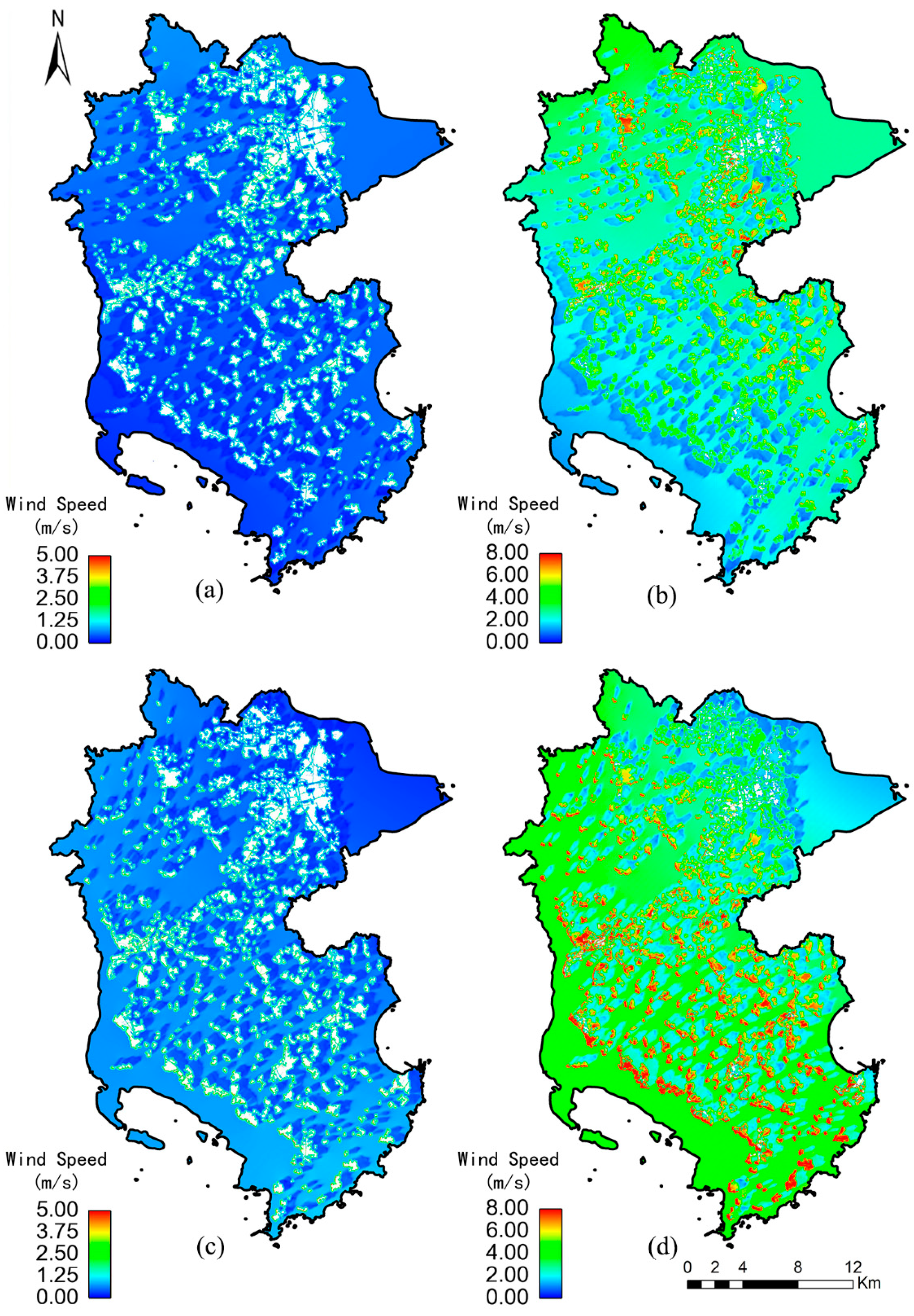
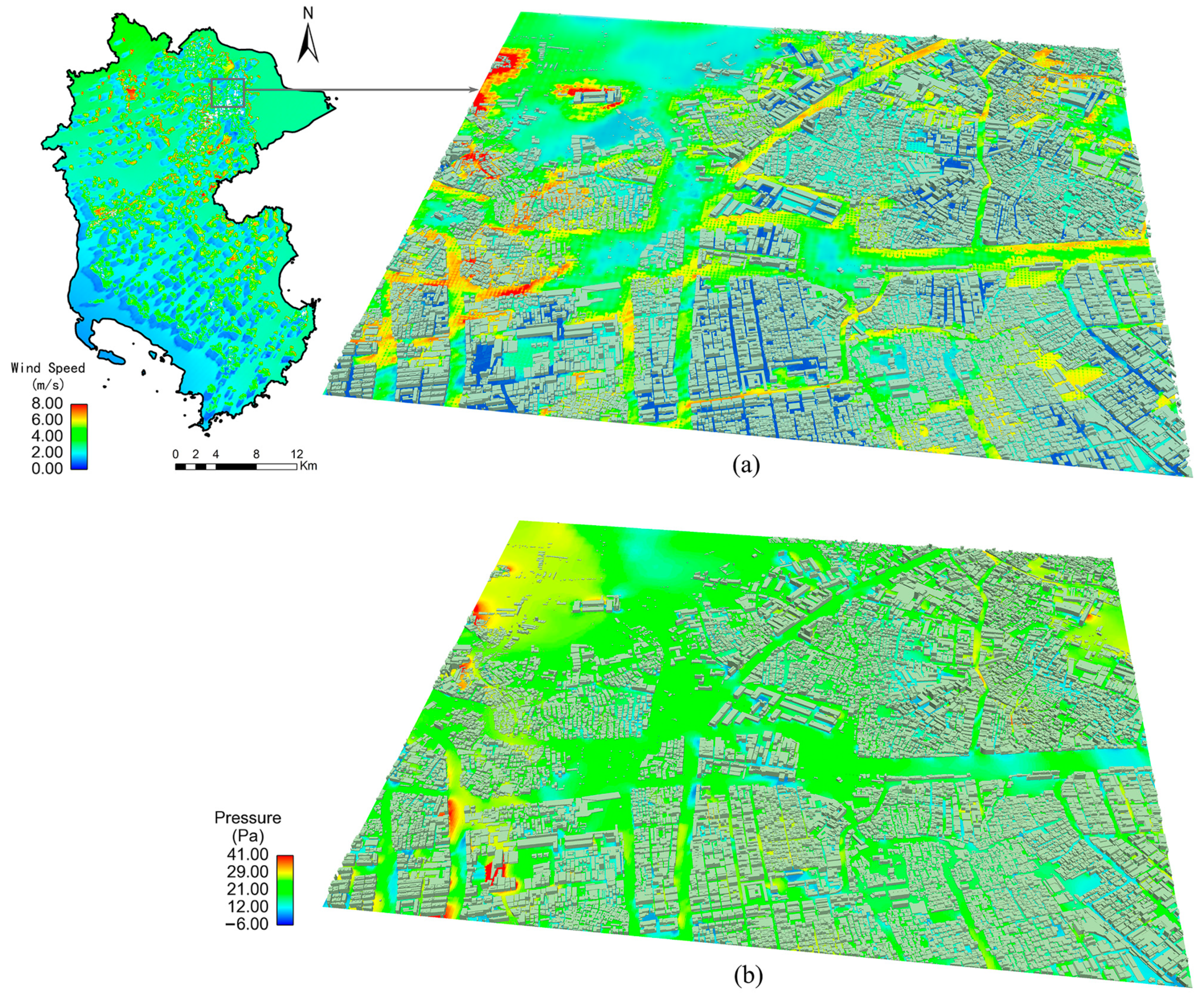
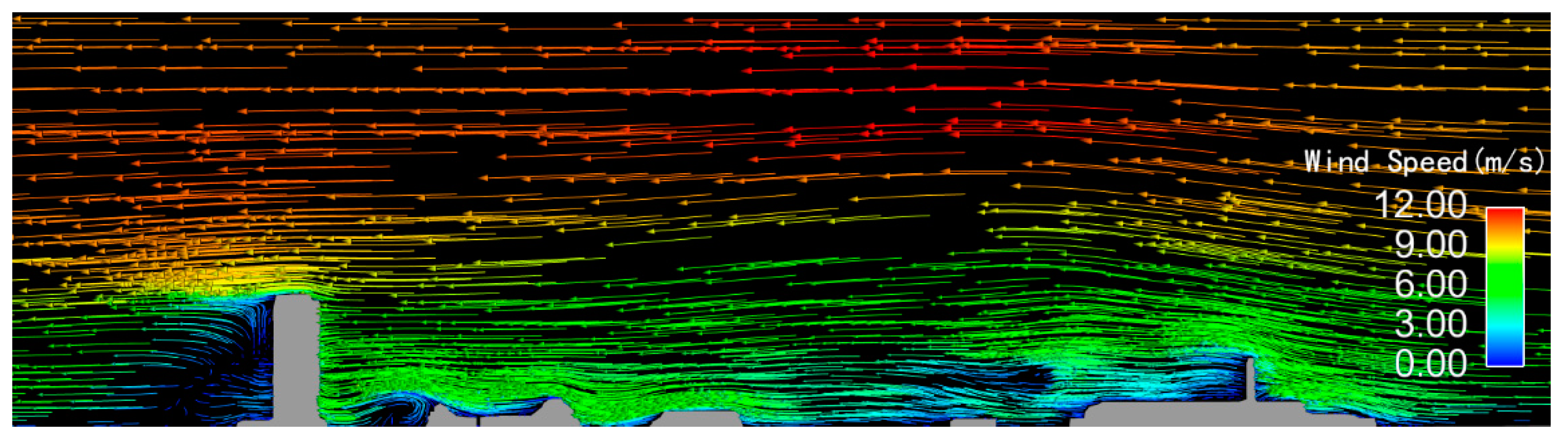
3.2. Simulation Results

To express the wind field characteristics at different heights and the 3D characteristics of the wind field, Ensight post-processing software was used for post-processing, and the outputs were the horizontal section wind speed diagram and the vertical section wind vector diagram.

Figure 8 shows the simulated results for the wind speed of a typical wind field in Jinjiang City. The wind speed in Jinjiang at a height of 2 m was relatively low, and the wind speed value was concentrated at 0–1.5 m/s. The windward side of the building groups had a relatively high wind speed. In the case of the dominant wind direction (NE), a relatively high wind speed appeared near the northeastern edge of the building groups and the central blocks, while in the case of the subdominant wind direction (SW), a high wind speed mainly appeared on the southwest side of the building area. At the 10 m height, the wind speed in the whole area of Jinjiang increased, and in some areas, it reached more than 5 m/s. The relatively high wind speed appeared near the windward side of the building. In the case of the dominant wind direction (NE), the high wind speed appeared on the northeast side of the building, and the low wind speed appeared in the southwestern part of the city, as well as in the densely constructed central city area in the northeast. In the case of the subdominant wind direction (SW), the high wind speed appeared on the southwest side of the buildings. The wind speed at the windward side of buildings in the central and southern regions of the city was relatively high. After being occluded by dense buildings in the northeastern part of the city, an obvious low wind speed zone was formed on the leeward side of the building near the northeast beach.

Figure 9 shows the simulated wind speed and static pressure of the NE case in the partial enlargement area at 10 m height. From the partially enlarged view of the wind speed simulation map (Figure 9a), it could be seen that the wind speed on the windward side of the building groups was significantly greater than that in other areas. In the leeward direction of the buildings, a wind shadow area was formed. The larger the frontal area of the building, the larger the wind shadow area. The wind occlusion of the buildings was obvious. The inner enveloping area and the leeward side of the building groups had obvious low wind speed characteristics. However, in some areas, the building was generally less than 10 m high. Even if the number of buildings in this area was large, the wind speed at the height of 10 m was relatively high. At the top of the roads that followed the wind direction and their associated road intersections, the wind speed was higher than that of the adjacent buildings, and these roads acted as ventilation corridors. However, on some narrow curved roads, the increase in wind speed was not obvious, which also indicated that the corridor needs to be wide enough to promote urban ventilation. This phenomenon was consistent with the general rule that wind flowed around buildings. Figure 9b shows the simulated static pressure of the NE case in the partial enlargement area at 10 m height. The value of static pressure was expressed as the relative static pressure, i.e., the difference from the standard atmospheric pressure (1013.25 hPa). It can be seen from Figure 9b that the high value area of static pressure was mostly located on the east side and north side of the building groups and the above road, while the low value area was mostly located on the west side and south side of the building groups, especially the enclosed area. The static pressure was relatively uniform on the wide roads whose directions were similar with the dominant wind direction, and near the windward side and leeward side of the building groups usually appeared a relatively obvious wind pressure difference. The air flowed from one side of the building groups to the other due to the difference in wind pressure between the different areas around the building groups.

The simulated wind vector of a vertical section in the dominant wind direction case (NE) (Figure 10) shows that the high-altitude wind speed was greater than the surface wind speed and that the wind speed of the space increased with height overall. There was a rising air phenomenon when the wind passed through the building groups. When wind blew through the building groups, the wind speed gradually decreased, and a cavity area with very low wind speed appeared at the leeward side of the building group. Different building heights and architectural forms had different effects on the wind field. The higher the building was, the higher the altitude level that the building could affect. In the vicinity of high-rise buildings, the local flow fields’ rising air and subsiding air phenomenon was significant and had a wide range of influence. However, in the vicinity of the low-rise buildings, the abovementioned phenomenon had a small influence range and basically did not affect the high-altitude wind field. The above results show that the simulation predicted the phenomenon of rising and subsiding in flow circulation around buildings. From the characteristics of the buildings affecting the wind, the simulation results had the opportunity to be compared with experimental observations.

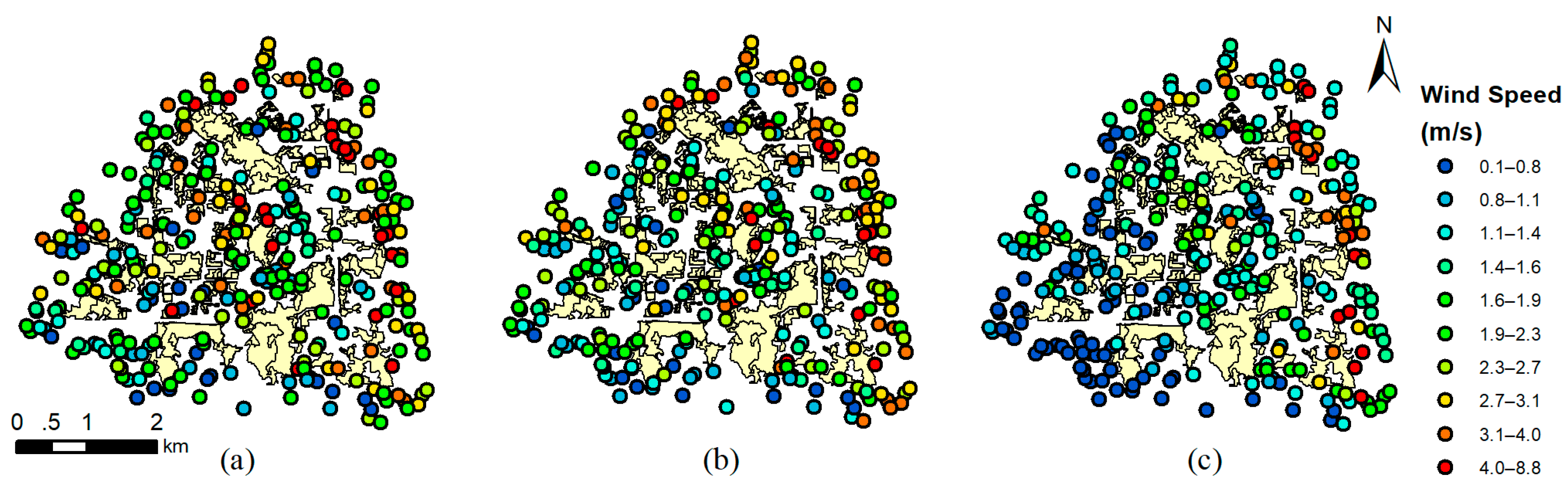
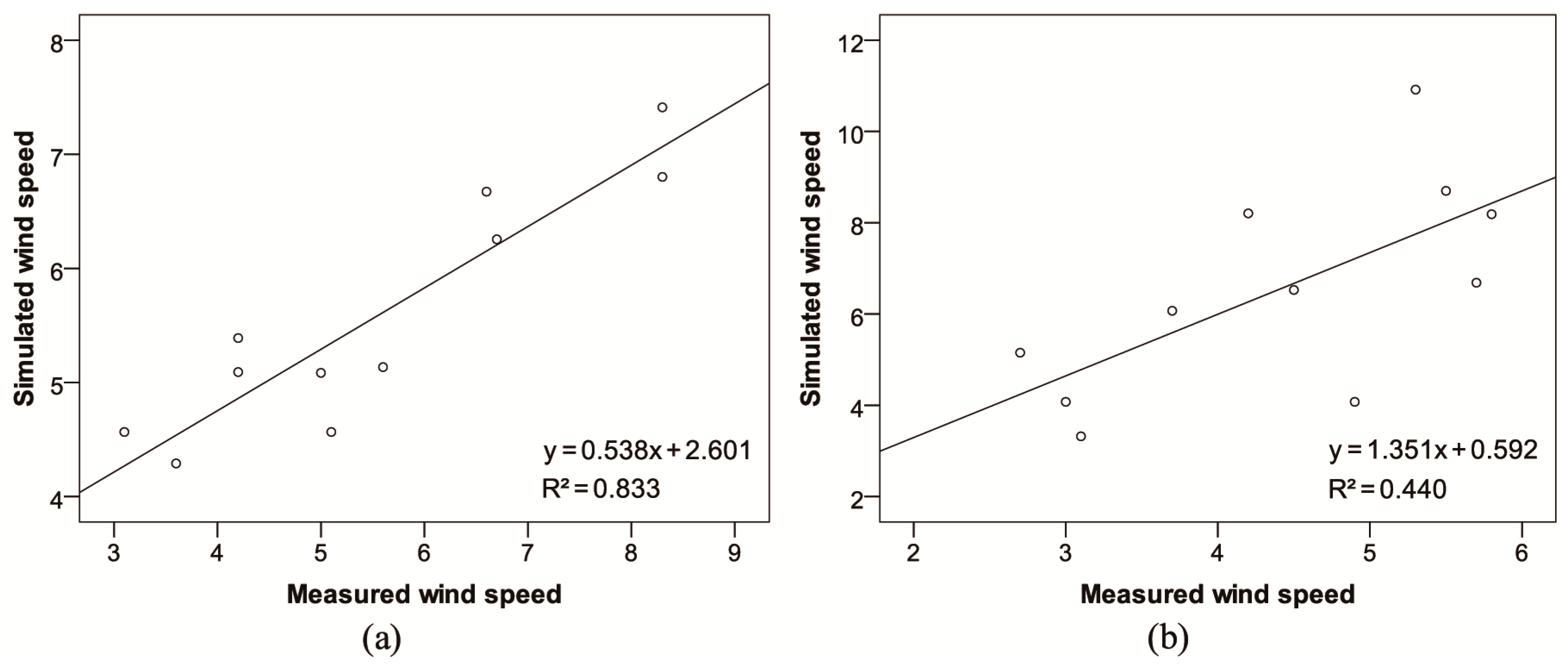
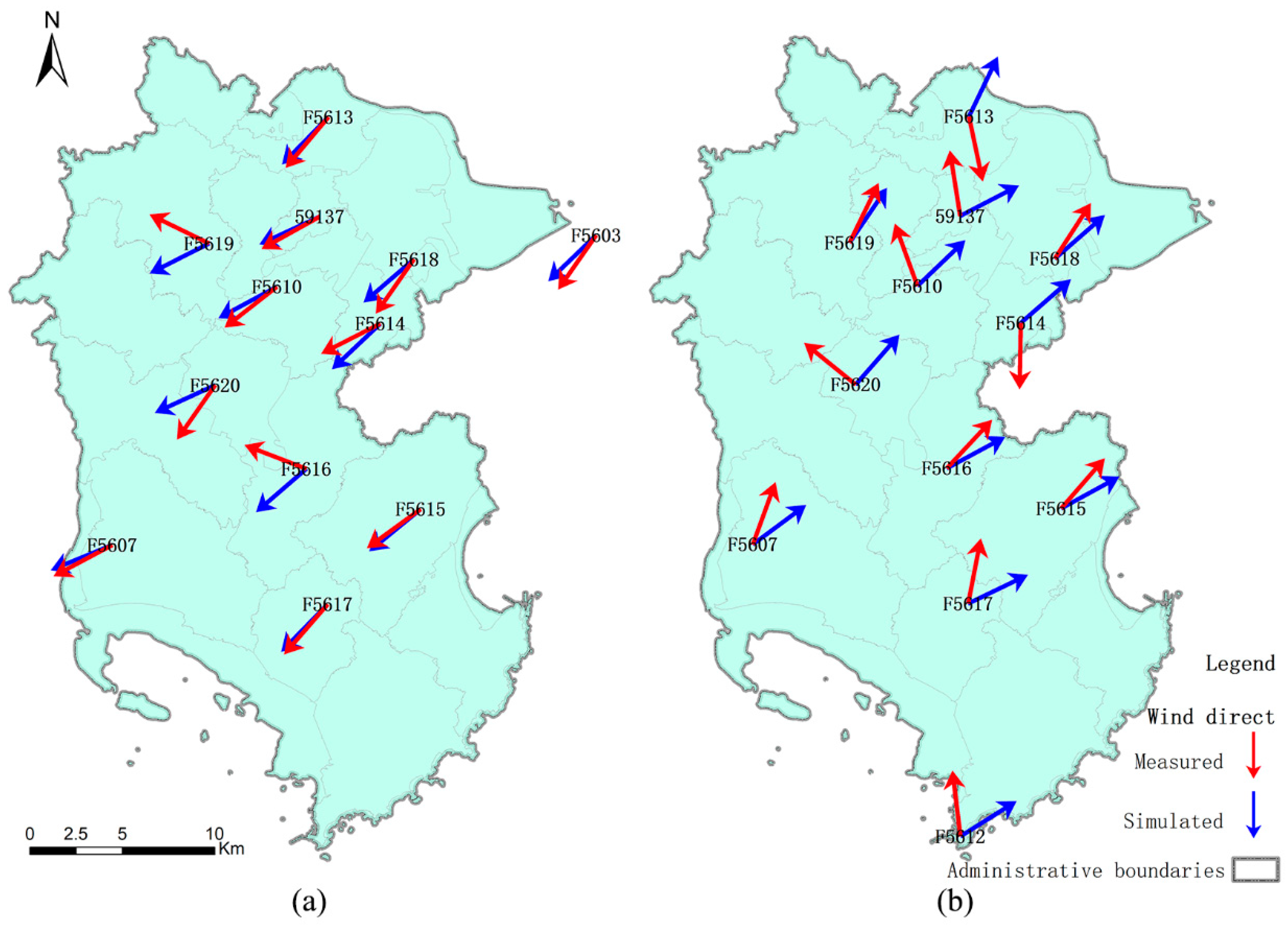
3.3. Comparison of Simulated and Measured Data

In this paper, the typical wind fields under average wind speed were simulated, but due to the complexity and transient characteristics of wind, it was difficult to compare the multiyear average data with the simulation results. If there was a realistic wind field situation with an inlet wind speed and direction similar to the simulation settings, if the wind speed of each meteorological station had a significant correlation with the simulation results, and if the station wind direction was similar to the simulation result, the simulation result could be considered as a reference for practical applications.

In order to evaluate the reliability of typical wind field simulation results, when the inflow wind speed and direction in the simulation were similar to the measured data of a station located in an upwind suburb of the city, the correlation and difference between the measured data and simulation results inside the city were analyzed. The time for which to use the observation data that were used was selected according to the wind speed and direction of the windward direction of the city. Observations from Jinjiang national station and regional automatic stations were used to compare with the simulation results (Figure 2). After field inspection, trees, air conditioners, etc., existed near some automatic stations, which made these local factors rather than urban architectural forms became the main influencing factors for the wind speed and direction of the stations. These sites were excluded from the comparison, as the simulations focused on the overall wind field of cities under the influence of buildings and without considering local factors such as vegetation. The regional automatic station F5603 was selected as the NE inlet flow wind approximation station, and the regional automatic station F5612 was the SW inlet flow wind approximation station. Typical wind fields under average wind speed were simulated in this paper. However, the multi-time average data of stations represented the average situation of multiple wind fields rather than a typical wind field. It was not appropriate to compare the simulation results with the multi-time average wind field. Therefore, a time was chosen for each typical wind field for comparison. The two stations’ wind conditions were used to select the measured wind field at specific times. After screening, the wind field at 11:00 on 9 January 2014, was selected for comparison with the dominant wind direction (NE), and the wind field at 8:00 on 18 June 2011, was selected for comparison with the subdominant wind direction (SW).

The wind speed simulation result and the measured value of the wind field cases for the dominant and subdominant wind directions (NE and SW) were statistically analyzed. The correlation between the simulated and measured values was analyzed, and the Pearson correlation test result was obtained (

Table 4. Pearson correlation test results of wind speed simulated and measured value.

Statistic	NE Case	SW Case
Correlation coefficient	0.913	0.663
Significance (bilateral)	8.807 × 10−5	0.026

). The wind speed correlation coefficient of the NE case was 0.913, and the significance (p value) was 8.807 × 10⁻⁵, indicating that the simulated value and the measured value were significantly correlated on both sides at the 0.01 level in this case. The wind speed correlation coefficient of the SW case was 0.663, and the significance (p value) was 0.026, indicating that the simulated value and the measured value in this case were significantly correlated on both sides at the 0.05 level. In both typical wind fields, the simulation results had a significant correlation with the measured values, indicating that the simulation results had practical rationality. From the statistical results, the correlation between the simulated value and the measured value in the case of the dominant wind direction was higher than that in the case of the subdominant wind direction. A possible reason for this phenomenon is that the actual wind field close to the NE case mainly occurs in winter, spring and autumn, while the actual wind field close to the SW case mainly appears in summer. The weather in summer is changeable, and the air convection is relatively strong. Compared with winter, the wind is more local and transient in summer, and the actual inflow speed and direction are also more uneven. It is more difficult to simulate the typical wind field with uniform inflow.

To quantitatively analyze the numerical difference between the simulated wind speed and the measured wind speed, the simulated and measured wind speeds of the dominant and subdominant wind direction (NE and SW) cases were analyzed by regression analysis (Figure 11). In both cases, the site simulation value and the measured value of the wind speed were basically linear. The coefficient of determination (R²) of the NE case was 0.833, and the linear regression equation had a high reference value. The R² of the SW case was 0.440, and the linear regression equation had a reference value. In both cases, the wind speed simulation values were overestimated. The smaller the measured wind speed value was, the more obvious the overestimation phenomenon in the NE case, and whereas a greater measured wind speed led to more obvious overestimation in the SW case. Generally, there was a linear correlation between the simulated and measured values of wind speed in both cases. The results could be used as a reference, but the specific values still deviated and were generally overestimated. The wind speed simulation value of the NE case had a relatively good correlation, and the linear correlation between the simulated and measured value of the SW case was slightly weaker than that of the NE case.

To analyze the difference between the simulation wind direction and the measured wind direction, the weather station simulation and measured wind direction of the dominant wind direction (NE) and the subdominant wind direction (SW) cases were compared. Figure 12 shows that in the NE case, the simulated wind direction had different amplitude deflections based on the inflow direction (NE). The simulated wind direction of most stations was very close to the measured wind direction, showing the NE, NNE or ENE direction. However, in individual stations such as regional automatic stations F5619 and F5616, the measured wind direction was quite different from that of the other stations. The simulated wind direction had a relatively low approximation of the measured wind direction at these stations. In the SW case, the simulated wind direction was generally SW, SSW or WSW, and it had different amplitude deflections based on the inflow direction (SW). The wind direction measured values were mostly in the vicinity of the SW wind direction values. However, compared with the NE case, the measured values of the wind direction of the WS case were quite varied, and wind directions such as NW and SE appeared. For some stations, such as regional automatic stations F5613 and F5614, the measured wind direction was quite different from that of the other stations, and the simulated wind direction result cannot be effectively approximated to match the measured wind direction.

A comprehensive comparison between the simulation results and the measured wind speed and wind direction shows that there was a significant correlation between the wind speed simulation values and the measured values. The simulated wind direction was consistent with the measured wind direction of most weather stations, except for the stations where the difference between the measured wind direction and the macro wind direction was relatively large. The simulated wind speeds of the two typical wind fields were overestimated. The correlation between the simulated wind speed and the measured values of the subdominant wind direction was weaker than that with the dominant wind direction. This indicates that both the simulated wind speed and the simulated wind direction could provide a reference, but further research is needed to fully address these problems.

4. Discussion

In this paper, a new building data generalization method was developed. It was a new approach to achieve high efficiency simulations of the city's overall wind field. Using the method, an overall CFD simulation of the urban-scale wind field was realized. Additionally, the simulation speed was improved and the workload was reduced while retaining the original distribution of the buildings. The simulation results were detailed and intuitive.

In order to maximize the improvement of the computational efficiency in the study, the most computationally efficient models and algorithms were often used in the discretization and solution of CFD, and the standard of simulation fineness was relatively low. For example, temperature change and heat exchange was ignored; diurnal variation in wind speed and direction was not considered and the standard k-ε model was the only employed turbulence model. This approach was consistent with the goal of quickly understanding urban ventilation in a low-cost manner, but ignored many processes in the real world.

In reality, when the wind is slightly disturbed, it will produce large local differentiations. Additionally, local temperature and radiation also affect air flow. The simulation results, especially the simulated wind direction, still had some deviation from the measured values. Thus, in follow-up studies, we will try to apply more turbulence models and meshing methods under the premise of computational efficiency or use the measured data to further correct the simulation results by means of spatial interpolation so that the simulation results are more in line with the actual wind field. We will compare the calculation results and efficiency of different meshing methods and turbulence models. We will also consider temperature, solar radiation and diurnal variation of wind to simulate a more realistic urban environment. In subsequent applications, factors such as terrain and vegetation that affect the urban wind environment will also be considered to obtain simulation results that are more similar to the actual situation. We will also consider combining the CFD simulation using the building data generalization method with the mesoscale climate model simulation results to study the actual wind field at a specific time under the influence of high altitude air disturbance.

5. Conclusions

In this paper, based on GIS technology, a building data generalization method was developed to solve the problems of a large amount of data and calculation in urban-scale CFD wind field simulations. Using Fluent software, high-precision urban building geographic information data and elevation attribute data, the method was applied to Jinjiang City, Fujian Province, China, a city of approximately 722 square km. A CFD numerical simulation of the wind field of Jinjiang City was implemented, and detailed and intuitive wind field information was obtained. Then, the simulation results were compared with the measured data.

The research shows the following: (1) The generalization method of building data could reduce the geometric model data volume and improve the modeling efficiency without changing the macroscopic distribution characteristics of building groups. With the method, an overall CFD wind field simulation study at the urban scale could be realized. (2) In the simulation results of two typical wind fields, the simulated wind field near buildings predicted the phenomenon of rising and subsiding in flow circulation around buildings. Given the characteristics of the wind affected by the buildings, the simulation results had rationality. (3) The wind speed simulation results for the dominant (NE) and subdominant (SW) wind direction cases were significantly correlated with the measured values. The simulated wind speeds of the two cases were both overestimated, and the correlation between the simulated and measured wind speeds of the SW case was weaker than that of the NE case. The simulated wind direction was consistent with that found at most of the measured stations. The simulated wind direction of the NE case was more approximate to the measured wind direction than that of the SW case. Both the simulated wind speed and the simulated wind direction could provide a reference.

To summarize, urban-scale wind field numerical simulation using the CFD approach and urban building geographic information data is feasible in terms of cost and efficiency when using the building data generalization method based on GIS. The simulation results can directly reflect the 3D wind field information in the city and provide a reference for understanding the urban wind environment.

References

1. Oke, T.R. Urban climate and global environmental change. In Applied Climatology Principles & Practices; Rutledge: London, UK, 1997; pp. 273–287. [Google Scholar]
2. Yang, J.; Zhang, T. Coupling Mechanism between Wind Environment and Space Form and Optimization Design in City Center; Southeast University Press: Nanjing, China, 2016; p. 2. [Google Scholar]
3. Howard, L. The Climate of London: Deduced from Meteorological Observations, Made at Different Places in the Neighbourhood of the Metropolis; W. Phillips: Cambridge, MA, USA, 1820; Volume 1. [Google Scholar]
4. Stathopoulos, T.; Storms, R. Wind environmental conditions in passages between buildings. J. Wind Eng. Ind. Aerodyn. 1986, 24, 19–31. [Google Scholar] [CrossRef]
5. Murakami, S.; Iwasa, Y.; Morikawa, Y. Study on acceptable criteria for assessing wind environment at ground level based on residents’ diaries. J. Wind Eng. Ind. Aerodyn. 1986, 24, 1–18. [Google Scholar] [CrossRef]
6. To, A.; Lam, K.M. Evaluation of pedestrian–level wind environment around a row of tall buildings using a quartile–level wind speed descripter. J. Wind Eng. Ind. Aerodyn. 1995, 54, 527–541. [Google Scholar] [CrossRef]
7. White, B.R. Analysis and wind–tunnel simulation of pedestrian–level winds in San Francisco. J. Wind Eng. Ind. Aerodyn. 1992, 44, 2353–2364. [Google Scholar] [CrossRef]
8. Kubota, T.; Miura, M.; Tominaga, Y.; Mochida, A. Wind tunnel tests on the relationship between building density and pedestrian–level wind velocity: Development of guidelines for realizing acceptable wind environment in residential neighborhoods. Build. Environ. 2008, 43, 1699–1708. [Google Scholar] [CrossRef]
9. Livesey, F.; Inculet, D.; Isyumov, N.; Davenport, A. A scour technique for the evaluation of pedestrian winds. J. Wind Eng. Ind. Aerodyn. 1990, 36, 779–789. [Google Scholar] [CrossRef]
10. Murakami, S.; Ooka, R.; Mochida, A.; Yoshida, S.; Kim, S. CFD analysis of wind climate from human scale to urban scale. J. Wind Eng. Ind. Aerodyn. 1999, 81, 57–81. [Google Scholar] [CrossRef]
11. Sofotasiou, P.; Hughes, B.; Ghani, S.A. CFD optimisation of a stadium roof geometry: A qualitative study to improve the wind microenvironment. Sustain. Build. 2017, 2, 8. [Google Scholar] [CrossRef]
12. Soltani, M.; Dehghani–Sanij, A.; Sayadnia, A.; Kashkooli, F.; Gharali, K.; Mahbaz, S.; Dusseault, M. Investigation of airflow patterns in a new design of wind tower with a wetted surface. Energies 2018, 11, 1100. [Google Scholar] [CrossRef]
13. Chan, A.T.; Au, W.T.W.; So, E.S.P. Strategic guidelines for street canyon geometry to achieve sustainable street air quality–part II: Multiple canopies and canyons. Atmos. Environ. 2003, 37, 2761–2772. [Google Scholar] [CrossRef]
14. Letzel, M.O.; Krane, M.; Raasch, S. High resolution urban large–eddy simulation studies from street canyon to neighbourhood scale. Atmos. Environ. 2008, 42, 8770–8784. [Google Scholar] [CrossRef]
15. Yuan, C.; Ng, E. Building porosity for better urban ventilation in high-density cities–A computational parametric study. Build. Environ. 2012, 50, 176–189. [Google Scholar] [CrossRef]
16. Yuan, C.; Ng, E. Practical application of CFD on environmentally sensitive architectural design at high density cities: A case study in Hong Kong. Urban Clim. 2014, 8, 57–77. [Google Scholar] [CrossRef]
17. Ai, Z.T.; Mak, C.M. CFD simulation of flow in a long street canyon under a perpendicular wind direction: Evaluation of three computational settings. Build. Environ. 2017, 114, 293–306. [Google Scholar] [CrossRef]
18. Shirzadi, M.; Naghashzadegan, M.A.; Mirzaei, P. Improving the CFD modelling of cross–ventilation in highly–packed urban areas. Sustain. Cities Soc. 2018, 37, 451–465. [Google Scholar] [CrossRef]
19. Zhang, A.; Gao, C.; Zhang, L. Numerical simulation of the wind field around different building arrangements. J. Wind Eng. Ind. Aerodyn. 2005, 93, 891–904. [Google Scholar] [CrossRef]
20. He, J.; Song, C.C.S. Evaluation of pedestrian winds in urban area by numerical approach. J. Wind Eng. Ind. Aerodyn. 1999, 81, 295–309. [Google Scholar] [CrossRef]
21. Tominaga, Y.; Mochida, A.; Yoshie, R.; Kataoka, H.; Nozu, T.; Yoshikawa, M.; Shirasawa, T. AIJ guidelines for practical applications of CFD to pedestrian wind environment around buildings. J. Wind Eng. Ind. Aerodyn. 2008, 96, 1749–1761. [Google Scholar] [CrossRef]
22. Peng, C.; Ming, T.; Cheng, J.; Wu, Y.; Peng, Z.R. Modeling thermal comfort and optimizing local renewal strategies–A case study of dazhimen neighborhood in Wuhan city. Sustainability 2015, 7, 3109–3128. [Google Scholar] [CrossRef]
23. Toparlar, Y.; Blocken, B.; Vos, P.; Van Heijst, G.J.F.; Janssen, W.D.; Van Hooff, T.; Montazeri, H.; Timmermans, H.J.P. CFD simulation and validation of urban microclimate: A case study for Bergpolder Zuid, Rotterdam. Build. Environ. 2015, 83, 79–90. [Google Scholar] [CrossRef] [Green Version]
24. Wise, D.J.; Boppana, V.B.L.; Li, K.W.; Poh, H.J. Effects of minor changes in the mean inlet wind direction on urban flow simulations. Sustain. Cities Soc. 2018, 37, 492–500. [Google Scholar] [CrossRef]
25. Eliasson, I.; Offerle, B.; Grimmond, C.S.B.; Lindqvist, S. Wind fields and turbulence statistics in an urban street canyon. Atmos. Environ. 2006, 40, 1–16. [Google Scholar] [CrossRef]
26. Stathopoulos, T.; Baskaran, B.A. Computer simulation of wind environmental conditions around buildings. Eng. Struct. 1996, 18, 876–885. [Google Scholar] [CrossRef]
27. Rafailidis, S. Influence of building areal density and roof shape on the wind characteristics above a town. Bound. Layer Meteorol. 1997, 85, 255–271. [Google Scholar] [CrossRef]
28. Blocken, B.; Janssen, W.D.; Van Hooff, T. CFD simulation for pedestrian wind comfort and wind safety in urban areas: General decision framework and case study for the Eindhoven University campus. Environ. Model. Softw. 2012, 30, 15–34. [Google Scholar] [CrossRef]
29. Gousseau, P.; Blocken, B.; Stathopoulos, T.; Van Heijst, G.J.F. CFD simulation of near-field pollutant dispersion on a high–resolution grid: A case study by LES and RANS for a building group in downtown Montreal. Atmos. Environ. 2011, 45, 428–438. [Google Scholar] [CrossRef]
30. Mochida, A.; Murakami, S.; Ojima, T.; Kim, S.; Ooka, R.; Sugiyama, H. CFD analysis of mesoscale climate in the Greater Tokyo area. J. Wind Eng. Ind. Aerodyn. 1997, 67–68, 459–477. [Google Scholar] [CrossRef]
31. Jiménez, P.A.; González–Rouco, J.F.; García–Bustamante, E.; Navarro, J.; Montávez, J.P.; De Arellano, J.V.G.; Dudhia, J.; Muñoz–Roldan, A. Surface wind regionalization over complex terrain: Evaluation and analysis of a high–resolution WRF simulation. J. Appl. Meteorol. Climatol. 2010, 49, 268–287. [Google Scholar] [CrossRef]
32. Salamanca, F.; Martilli, A.; Tewari, M.; Chen, F. A study of the urban boundary layer using different urban parameterizations and high–resolution urban canopy parameters with WRF. J. Appl. Meteorol. Climatol. 2011, 50, 1107–1128. [Google Scholar] [CrossRef]
33. Liu, Y.S.; Miao, S.G.; Zhang, C.L.; Cui, G.X.; Zhang, Z.S. Study on micro–atmospheric environment by coupling large eddy simulation with mesoscale model. J. Wind Eng. Ind. Aerodyn. 2012, 107–108, 106–117. [Google Scholar] [CrossRef]
34. Jiménez, P.A.; Dudhia, J. On the ability of the WRF model to reproduce the surface wind direction over complex terrain. J. Appl. Meteorol. Climatol. 2013, 52, 1610–1617. [Google Scholar] [CrossRef]
35. Soares, P.M.M.; Cardoso, R.M.; Miranda, P.M.A.; De Medeiros, J.; Belo–Pereira, M.; Espirito–Santo, F. WRF high resolution dynamical downscaling of ERA–Interim for Portugal. Clim. Dyn. 2012, 39, 2497–2522. [Google Scholar] [CrossRef]
36. Baik, J.J.; Park, S.B.; Kim, J.J. Urban flow and dispersion simulation using a CFD model coupled to a mesoscale model. J. Appl. Meteorol. Climatol. 2009, 48, 1667–1681. [Google Scholar] [CrossRef]
37. Chen, F.; Kusaka, H.; Bornstein, R.; Ching, J.; Grimmond, C.S.B.; Grossman–Clarke, S.; Loridan, T.; Manning, K.W.; Martilli, A.; Miao, S.; et al. The integrated WRF/urban modelling system: development, evaluation, and applications to urban environmental problems. Int. J. Climatol. 2011, 31, 273–288. [Google Scholar] [CrossRef]
38. Miao, Y.; Liu, S.; Chen, B.; Zhang, B.; Wang, S.; Li, S. Simulating urban flow and dispersion in Beijing by coupling a CFD model with the WRF model. Adv. Atmos. Sci. 2013, 30, 1663–1678. [Google Scholar] [CrossRef]
39. José, R.S.; Pérez, J.L.; Pérez, L.; González Barras, R.M. Modelling of urban climate impacts using regional and urban CFD models. Application to madrid (Spain) and London (UK). In Proceedings of the 2017 Winter Simulation Conference, Las Vegas, NV, USA, 3–6 December 2017. [Google Scholar]
40. Murga, A.; Sano, Y.; Kawamoto, Y.; Ito, K. Integrated analysis of numerical weather prediction and computational fluid dynamics for estimating cross–ventilation effects on inhaled air quality inside a factory. Atmos. Environ. 2017, 167, 11–22. [Google Scholar] [CrossRef]
41. Mughal, M.O.; Lynch, M.; Yu, F.; Sutton, J. Forecasting and verification of winds in an East African complex terrain using coupled mesoscale–And micro-scale models. J. Wind Eng. Ind. Aerodyn. 2018, 176, 13–20. [Google Scholar] [CrossRef]
42. Yoshie, R.; Mochida, A.; Tominaga, Y.; Kataoka, H.; Harimoto, K.; Nozu, T.; Shirasawa, T. Cooperative project for CFD prediction of pedestrian wind environment in the Architectural Institute of Japan. J. Wind Eng. Ind. Aerodyn. 2007, 95, 1551–1578. [Google Scholar] [CrossRef]
43. Environmental Systems Research Institute (ESRI). ArcGIS Help 10.2, ESRI Inc.: Redlands, CA, USA, 2013.
44. Aliabadi, A.A.; Krayenhoff, E.S.; Nazarian, N.; Chew, L.W.; Armstrong, P.R.; Afshari, A.; Norford, L.K. Effects of roof–edge roughness on air temperature and pollutant concentration in urban canyons. Bound. Layer Meteorol. 2017, 164, 249–279. [Google Scholar] [CrossRef]
45. Blocken, B.; Stathopoulos, T.; Carmeliet, J. CFD simulation of the atmospheric boundary layer: Wall function problems. Atmos. Environ. 2007, 41, 238–252. [Google Scholar] [CrossRef]
46. Kays, W.M.; Crawford, M.E. Convective Heat and Mass Transfer, 3rd ed.; McGraw Hill Inc.: New York, NY, USA, 1993. [Google Scholar]
47. Aliabadi, A.A.; Veriotes, N.; Pedro, G. A Very Large–Eddy Simulation (VLES) model for the investigation of the neutral atmospheric boundary layer. J. Wind Eng. Ind. Aerodyn. 2018, 183, 152–171. [Google Scholar] [CrossRef]
48. Davenport, A.G. Rationale for determining design wind velocities. J. Struct. Div. 1960, 86, 39–68. [Google Scholar]
49. China Association for Engineering Construction Standardization (CECS). Load Code for the Design of Building Structures (GB50009-2012); China Architecture & Building Press: Beijing, China, 2012.
50. Xiaomin, X.; Zhen, H.; Jiasong, W. The impact of urban street layout on local atmospheric environment. Build. Environ. 2006, 41, 1352–1363. [Google Scholar] [CrossRef]
51. Kumar, P.; Garmory, A.; Ketzel, M.; Berkowicz, R.; Britter, R. Comparative study of measured and modelled number concentrations of nanoparticles in an urban street canyon. Atmos. Environ. 2009, 43, 949–958. [Google Scholar] [CrossRef] [Green Version]
52. Ramponi, R.; Blocken, B.; De Coo, L.B.; Janssen, W.D. CFD simulation of outdoor ventilation of generic urban configurations with different urban densities and equal and unequal street widths. Build. Environ. 2015, 92, 152–166. [Google Scholar] [CrossRef] [Green Version]
53. Hang, J.; Li, Y. Ventilation strategy and air change rates in idealized high–rise compact urban areas. Build. Environ. 2010, 45, 2754–2767. [Google Scholar] [CrossRef]
54. Fluent Inc. FLUENT 15.0 Theory Guide; Fluent Inc.: Canonsburg, PA, USA, 2013. [Google Scholar]
55. Giometto, M.G.; Christen, A.; Calaf, M.; Parlange, M. The impact of variable building height on drag, flow and turbulence over a realistic suburban surface. In Proceedings of the AGU General Assembly Conference, San Francisco, CA, USA, 9–14 February 2014. [Google Scholar]
Figure 1. Wind rose diagram of Jinjiang City in January, April, July and October.
Atmosphere 10 00326 g001
Figure 2. The spatial distribution of buildings in Jinjiang and the position of the comparison stations.
Atmosphere 10 00326 g002
Figure 3. Building data generalization flow chart.
Atmosphere 10 00326 g003
Figure 4. Computational domain.
Atmosphere 10 00326 g004
Figure 5. Simulated wind speed at the random points: (a) Case 1; (b) Case 2 and (c) Case 3.
Atmosphere 10 00326 g005
Figure 6. Comparison of building features before and after generalization: (a) Building features before generalization and (b) building features after generalization.
Atmosphere 10 00326 g006
Figure 7. Comparison of the quantities of buildings before and after generalization.
Atmosphere 10 00326 g007
Figure 8. Simulation wind speed of typical wind fields in Jinjiang: (a) 2 m height, NE case; (b) 10 m height, NE case; (c) 2 m height, SW case and (d) 10 m height, SW case.
Atmosphere 10 00326 g008
Figure 9. Simulation wind speed and static pressure of the NE case in Jinjiang at 10 m height (partial enlargement): (a) Simulation wind speed and (b) simulation static pressure; the grey blocks represent buildings.
Atmosphere 10 00326 g009
Figure 10. Simulated wind vector of a vertical section: Partial enlargement; the section in the figure is the Y-direction section, which was located in the northeast of the city.
Atmosphere 10 00326 g010
Figure 11. Typical wind field regression scatter plot: (a) NE case and (b) SW case.
Atmosphere 10 00326 g011
Figure 12. Comparison between simulated and measured wind directions at the meteorological stations: (a) NE case and (b) SW case; the arrow is pointing to the direction that the wind blows.
Atmosphere 10 00326 g012