The Effect of Increasing Surface Albedo on Urban Climate and Air Quality: A Detailed Study for Sacramento, Houston, and Chicago

Heat Island Group, Building, Civil and Environmental Engineering Department, Concordia University, Montreal, QC H3G 1M8, Canada
*
Author to whom correspondence should be addressed.
Climate 2018, 6(2), 19; https://0-doi-org.brum.beds.ac.uk/10.3390/cli6020019
Submission received: 28 January 2018
/
Revised: 15 March 2018
/
Accepted: 15 March 2018
/
Published: 21 March 2018
(This article belongs to the Special Issue Urban Overheating - Progress on Mitigation Science and Engineering Applications)
Abstract
:Increasing surface reflectivity in urban areas can decrease ambient temperature, resulting in reducing photochemical reaction rates, reducing cooling energy demands and thus improving air quality and human health. The weather research and forecasting model with chemistry (WRF-Chem) is coupled with the multi-layer of the urban canopy model (ML-UCM) to investigate the effects of surface modification on urban climate in a two-way nested approach over North America focusing on Sacramento, Houston, and Chicago during the 2011 heat wave period. This approach decreases the uncertainties associated with scale separation and grid resolution and equip us with an integrated simulation setup to capture the full impacts of meteorological and photochemical reactions. WRF-ChemV3.6.1 simulated the diurnal variation of air temperature reasonably well, overpredicted wind speed and dew point temperature, underpredicted relative humidity, overpredicted ozone and nitrogen dioxide concentrations, and underpredicted fine particular matters (PM2.5). The performance of PM2.5 is a combination of overprediction of particulate sulfate and underprediction of particulate nitrate and organic carbon. Increasing the surface albedo of roofs, walls, and pavements from 0.2 to 0.65, 0.60, and 0.45, respectively, resulted in a decrease in air temperature by 2.3 °C in urban areas and 0.7 °C in suburban areas; a slight increase in wind speed; an increase in relative humidity (3%) and dew point temperature (0.3 °C); a decrease of PM2.5 and O3 concentrations by 2.7 µg/m3 and 6.3 ppb in urban areas and 1.4 µg/m3 and 2.5 ppb in suburban areas, respectively; minimal changes in PM2.5 subspecies; and a decrease of nitrogen dioxide (1 ppb) in urban areas.
1. Introduction
Increasing urban albedo is a verifiable and repeatable heat island mitigation strategy to decrease urban temperatures, photochemical reaction rates, and pollution, thus improving human health and comfort [1,2]. Land use changes and anthropogenic heat emissions contribute to the urban heat island effect by increasing air temperature by 0.42 °C and 0.22 °C, respectively [3]. The reflectivity of surfaces in urban areas range from 0.1 to 0.2 and can be increased by use of high reflective materials on roofs, walls, and pavements [1,4]. The effects of surface modifications on urban climate and atmospheric conditions have been investigated in various regions and episodes. Salamanca and Martilli [5] have shown that a higher albedo decreases urban temperature by 1.5–2 °C during hot summer days in Madrid. Fallmann et al. [6,7] showed that increasing surface albedo lead to a decrease in 2-m air temperature and ozone concentrations by nearly 0.5 °C and 5–8% in urban areas of Stuttgart during the 2003 heat wave period. Touchaei et al. [8] showed a decrease in maximum air temperature, ozone (O3), and fine particulate matters (PM2.5) concentrations by up to 0.7 °C, 0.2 ppb, and 1.8 µg/m3, respectively by increasing surface albedo in Montreal during the 2005 heat wave period. Jandaghian et al. [9] showed that by increasing surface reflectivity during a rainy episode in summer 2009, the air temperature decreases by 0.2 °C, wind speed slightly increases, and relative humidity and precipitation decrease by 2.8% and 0.2 mm, respectively over Montreal.
Air-quality prediction models have been developed in response to the increased concerns regarding the effects of air quality on human health. The interaction between chemistry and meteorology is complicated. Meteorology has its effects on chemistry through temperature (increasing the chemical reactions, photolytic rates and biogenic emissions), cloud formation (affecting mixing, transformation, and scavenging of chemical compounds), precipitation (increasing the removal of trace gases and aerosols), radiation (affecting photolysis rates, isoprene emissions, and chemical reaction rates), wind speed and direction (affecting horizontal transport and vertical mixing of chemical species and aerosol emissions), planetary boundary layer (PBL) height (affecting pollutant concentrations). In turn, chemistry influences meteorology through aerosol (affecting radiation transfer, cloud life time and optical depth, boundary layer meteorology, precipitation, and scattering/absorption); ozone (affecting radiation and temperature); NOx, CO, and VOCs (as the precursor of O3 contributions to ozone radiative effects). Land surface properties also affect natural emission and dry deposition [10]. The online coupled weather research and forecasting model with chemistry (WRF-Chem) is developed to simulate meteorological quantities and air pollution concentrations simultaneously [11]. The model is a fully compressible, non-hydrostatic mesoscale numerical weather prediction (NWP) system. WRF-Chem has several physical and chemical parameterizations [12]. The component of air quality is consistent with the meteorological ones within the same transport scheme, grid and physics schemes, and time steps. The spatial and temporal aspects of WRF-Chem application have been analyzed in many studies through one-way approaches, in local, regional or global scales [13,14,15,16,17,18]. However, a two-way nested approach in WRF-Chem needs to be applied over a larger geographical area through regional and local scales to equip us with an integrated simulation setup to capture the full impacts of meteorological and photochemical reactions. This approach reduces the uncertainties associated with scale separation and grid resolution to investigate the effects of UHI and surface modifications on urban climate and air quality. The morphological, thermal, and micro-scale properties of the urban canopy are considered by coupling of the multi-layer of the urban canopy model (ML-UCM) [19] within WRF-ChemV3.6.1. Applying the multi-layer of the UCM is necessary when analyzing the urbanization impacts on regional climate [20].
The intent of this research is to investigate the effects of urban heat island and increasing surface albedo on meteorological parameters, such as 2-m air temperature, 10-m wind speed, dew point temperature and 2-m relative humidity, and air quality parameters; namely ozone, fine particulate matters, nitrogen dioxide (NO2), PM2.5 subspecies (particulate sulfate (SO42.5), particulate nitrate (NO32.5), and organic carbon (OC2.5) concentrations. The simulation domain covers North America with focus on three populated cities in the United States of America: Sacramento in California, Houston in Texas, and Chicago in Illinois. The simulation episode is during the 2011 heat wave period. On 17 July 2011, the heat wave event started over eastern Ontario, southern Quebec and northern New England. The intense heat moved eastwards and peaked on 22 July with Central Park in New York City breaking the record for the day at 40 °C, which was the hottest temperature the city had experienced in over three decades. The heat wave continued to intensify, with temperatures in north Texas exceeding 38 °C, most days, beginning in mid-June. By 23 July, the heat had intensified and reached to 45 °C. For the entire U.S., the 2011 heat wave period was the hottest in 75 years. The duration of the heat event was at the minimum of 7 days to a maximum of 69 days [21]. The paper structure is as follows: the methodology includes model description and simulation setup and surface modification approach, the results and analyses include model performance evaluation and estimating the effects of increasing surface reflectivity on urban climate and regional air quality, the discussion includes the limitations and assumptions of the study, the conclusion includes a summary of the study and future steps.
2. Methodology
2.1. Model Description and Simulation Setup
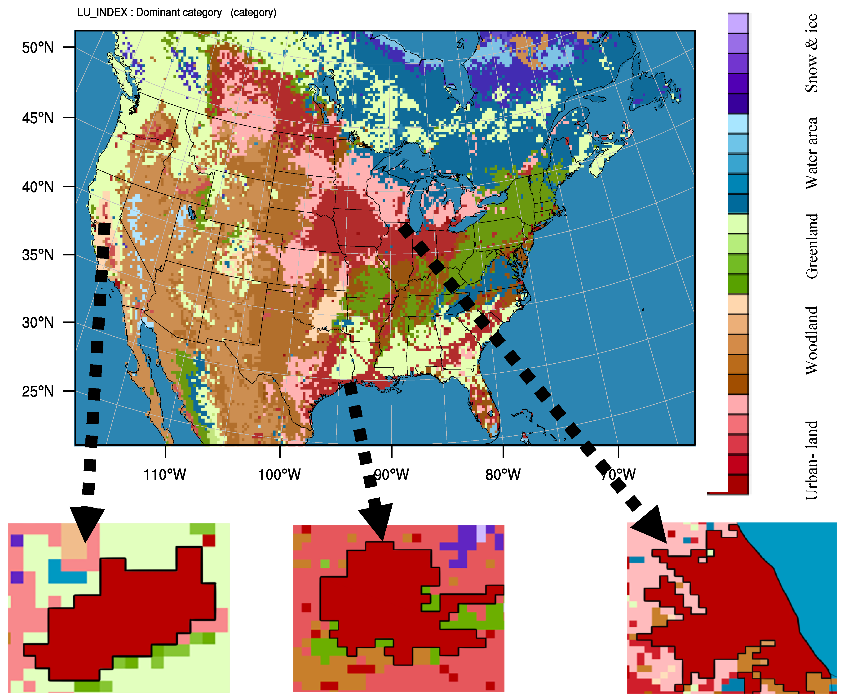
We used the online weather research and forecasting model with chemistry (WRF-Chem) and coupled it with the multi-layer of the urban canopy model (ML-UCM) to investigate the effects of urban heat island and its mitigation strategy over continental scale through urban scales during the 2011 heat wave period. The first domain covers North America (NA) including Canada, the United States, and the Northern part of Mexico with 445 grids in west–east direction and 338 grids in south–north direction. The horizontal resolution is 12 km. The second, third, and fourth domains cover the Sacramento area (36 × 31 grids), Houston area (41 × 31 grids), and Chicago area (36 × 31 grids) with the horizontal resolution of 2.4 km. The vertical resolution includes 35 vertical layers from the surface to a fixed pressure of ~100 mb (~16 km AGL). Figure 1 shows the simulation domains and land use/land cover. The simulation period extended over the seven consecutive hottest days in 2011, from the 17 to 23 July. We disregarded the first 72 h of the simulation as spin-up period.
The simulation is conducted with the initial and boundary conditions obtained from the North American Regional Reanalysis (NARR) [22,23] with a grid resolution of 32 km and a time resolution of 3-h. Land use was derived from the USGS 24-category data set. We used the Lin scheme as microphysics parameters to evaluate six classes of hydrometeors [24]. Goddard scheme [25] and rapid radiative transfer model (RRTMG; [26]) are respectively selected for shortwave and longwave radiations. The planetary boundary layer is simulated by the Mellor–Yamada–Janjic scheme using Eta similarity theory [27]. The unified Noah land surface model is applied as the land surface scheme. For cumulus parameterization, the Grell–Devenyi ensemble scheme [28] is used. We activated the positive-definite advections of moisture, scalars, and turbulent kinetic energy for model stability [29,30].
Modelling of the chemical compositions in the atmosphere, requires preliminary information concerning the emissions of chemical compounds within the modelling domain. We used the United States National Emission Inventory for 2011 (US-NEI11). The US-NEI11 contains the anthropogenic emissions of the U.S., southern Canada, and northern Mexico in 4-km spatial resolution, divided into point and area sources [31]. Guenther et al. [32] incorporated the quantitative understanding of biogenic emissions into a numerical model named Model of Emissions of Gases and Aerosols from Nature (MEGAN). MEGAN estimates the time resolved gridded BVOC emission estimation in mole/km2/h and is designed for regional and global emission simulations. The Modal Aerosol Dynamics Model for Europe (MADE) [33] is coupled with the chemistry package to evaluate the radiation and clouds interactions. Within WRF_Chem, the Regional Atmospheric Chemistry Mechanism (RACM) [34] is used for gas-phase reactions. The secondary organic aerosols (SOA) have been incorporated into MADE by means of the Secondary ORGanic Aerosol Model (SORGAM; [35]) Photolysis frequencies are calculated by the Fast_J model scheme [11,36,37,38,39]. Table 1 presents the physical and chemical parameterizations applied in WRF-ChemV3.6.1.
2.2. Increasing Surface Reflectivity
We conducted two sets of simulations with different scenarios concerning urban surface modifications: the base case condition that the albedo of roofs, walls, and pavements are assumed to be 0.2 (hereafter referred to as CTRL); and the increasing surface albedo scenario where the reflectivity of roofs, walls, and pavements is increased to 0.65, 0.60, and 0.45, respectively (hereafter referred to as ALBEDO). We selected three cities: Sacramento (CA), Houston (TX), and Chicago (IL) based on Akbari et al. [4,40,41,42] and Rose et al. [43] findings on the urban fabric of these cities. Using high-resolution orthophotography, they found that roofs cover 20–25% and pavements cover 30–40% of urban surfaces. Table 2 presents the urban fabric of Sacramento, Chicago, and Houston [43].
Here, we applied these fractions to characterize the fabric of the selected cities. Hence, the changes of surface albedo modification from the CTRL case as 0.2 to full adoption of roofs and pavements can be calculated as: 0.20 × 0.65 + 0.45 × 0.45 = 0.33 (as an example for Sacramento; an increase of 0.13 of roof albedo and 0.20 of pavement albedo on the urban scale). The change to gridded ALBEDO can be calculated as: (Surface albedo enhancement (roofs, walls, and pavements) × Fraction of urban areas per grid cell) [44].
3. Results and Analyses
3.1. Model Performance Evaluation
The local meteorological patterns affect the transport, transmission, advection, and diffusion of pollutants over the regional scale and further continental scales, which cannot be fully captured by the model to some extent [18]. We evaluated the model performance of WRF_ChemV3.6.1 by comparing the simulation results with observations obtained from weather and air-quality stations in Sacramento, Houston, and Chicago. The weather and air quality monitoring stations were chosen based on their locations close to the downtown of the selected cities (hereafter referred to as urban) and their surroundings (hereafter referred to as suburb). The hourly 2-m air temperature (T2), 10-m wind speed (WS10), 2-m relative humidity (RH2), and dew point temperature (Td) simulation results are compared with the measurements obtained from the U.S. Environmental Protection Agency (EPA) Clean Air Status and Trend Network (CASTNET). The daily averaged modelled fine particular matters (PM2.5), ozone (O3), nitrogen dioxide (NO2), PM2.5 subspecies (particulate sulfate (SO42.5), particulate nitrate (NO32.5), and organic carbon (OC2.5)) concentrations are compared with the EPA Air Quality System (AQS) observations using 24-h average data. [45,46,47,48,49]
Here, the time series of simulation results changed to the local time for each specific location: Sacramento: LST = UTC − 7 h; Houston and Chicago: LST = UTC − 5 h. The performance and accuracy of the simulation results are quantitatively based on a series of metrics estimations [50]. Here, we followed the Zhang et al. [51] calculations for the mean bias error (MBE), mean absolute error (MAE), and the root mean square error (RMSE) estimations of the meteorological and chemical parameters.
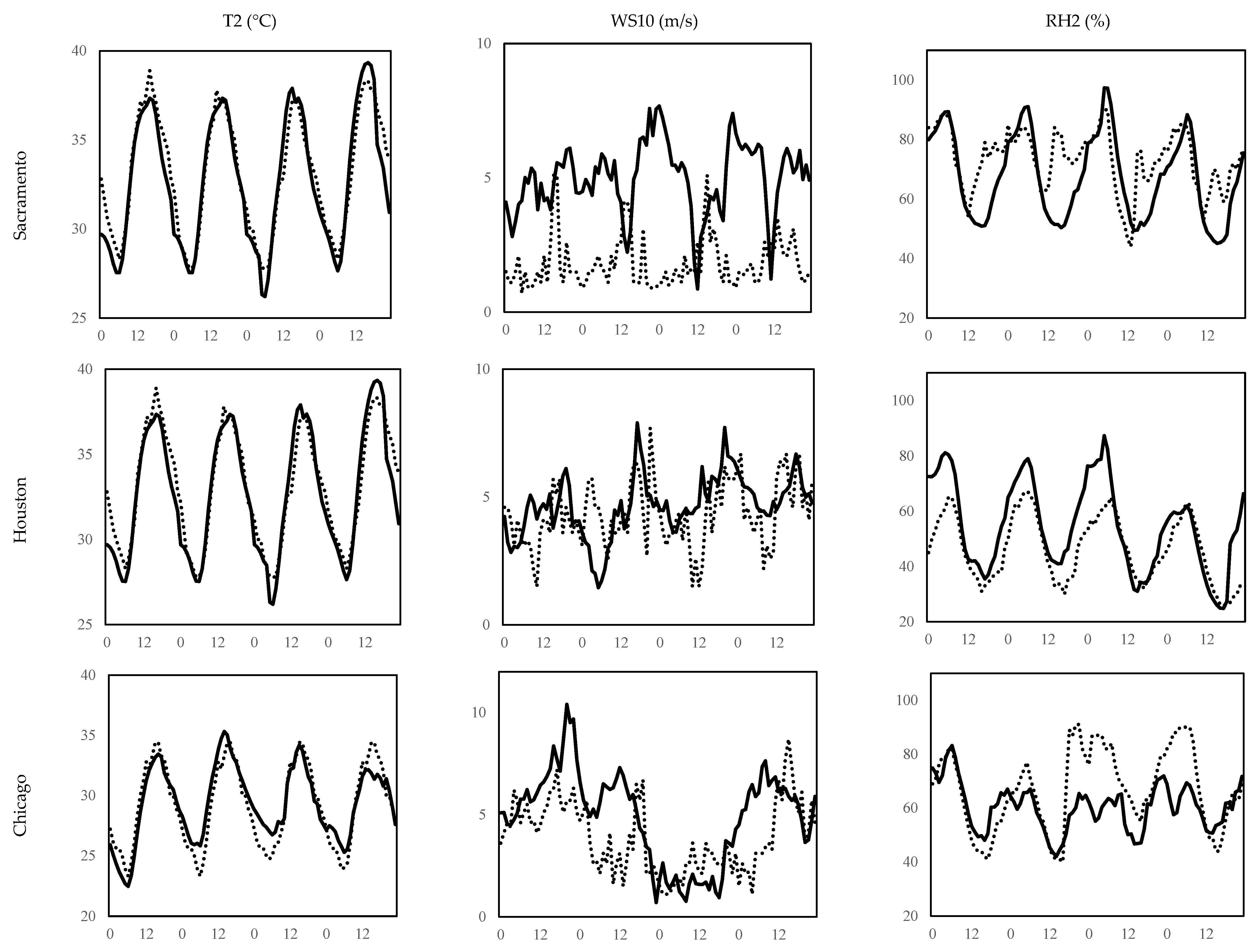
In terms of meteorological components of the model, the WRF-ChemV3.6.1 effectively captures the diurnal variations of 2-m air temperature, overpredicts 10-m wind speed, overpredicts dew point temperature, and underpredicts 2-m relative humidity. The MBA of T2 (−0.07 °C) shows that the model is capable in predicting air temperature. A small underprediction can be seen in urban areas (~−0.3 °C) that indicates the model deficiency in calculating the heat emission from anthropogenic sources in urban areas accurately. The MAE and RMSE of T2 are approximately 1 °C. Wind speed plays an important role in calculation of air temperature from skin temperature in the land surface model. The 10-m wind speed comparisons show small to large overpredictions (0.3 to 3.15 m/s). The MBA is 1.65 m/s, that shows the model is unable to capture the effects of micro scales and wind patterns. The MAE and RMSE of WS10 are almost 2 m/s. Relative humidity is a function of moisture content, air temperature, and surface pressure. The spatial distribution of RH2 represents an underestimation with the MBE of −1.42%. This underestimation shows that the microphysics scheme miscalculated the processes of transforming water (rain, vapor, cloud, etc.) and moisture fluxes. It also shows the model limitation in capturing the sea surface temperature, wind speed, and their impacts on water mixing ratio and water content of the air properly. The MAE and RMSE of RH2 are nearly 10% and 13%, respectively. Figure 2 shows the time series (hourly) of the observed vs. simulated T2 (°C), WS10 (m/s), and RH2 (%) in the urban areas of Sacramento, Houston, and Chicago. We also calculated the dew point temperature to avoid the dependency on air temperature for the moisture variable. The MBA, MAE, and RMSE of dew point temperature (0.39, 0.53, and 0.65 °C, respectively) show that the model overpredicts the moisture content in the atmosphere especially in urban areas (~0.5 °C).
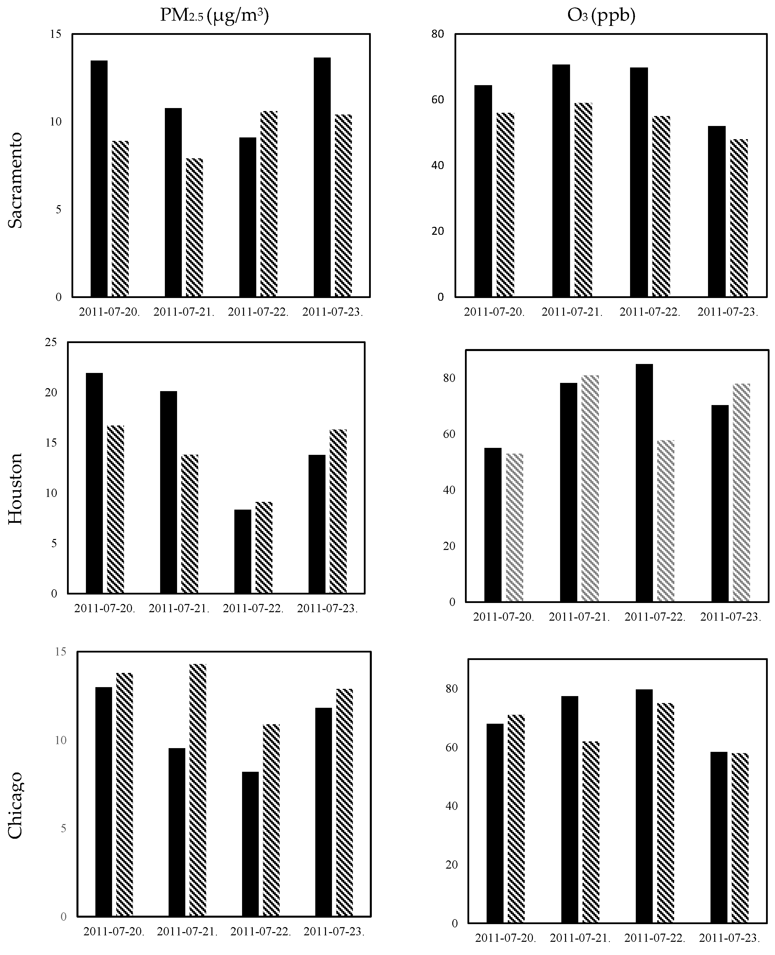
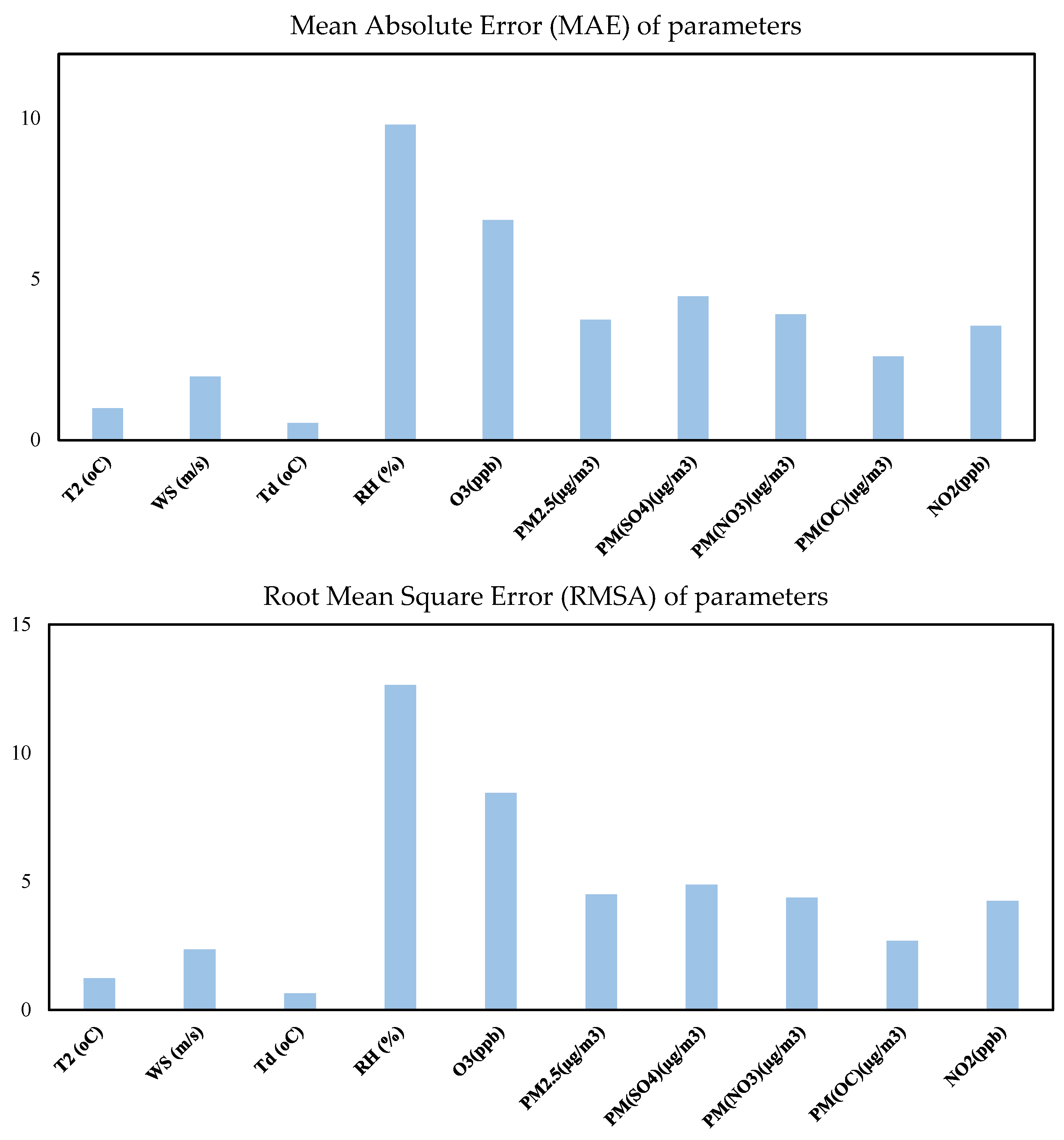
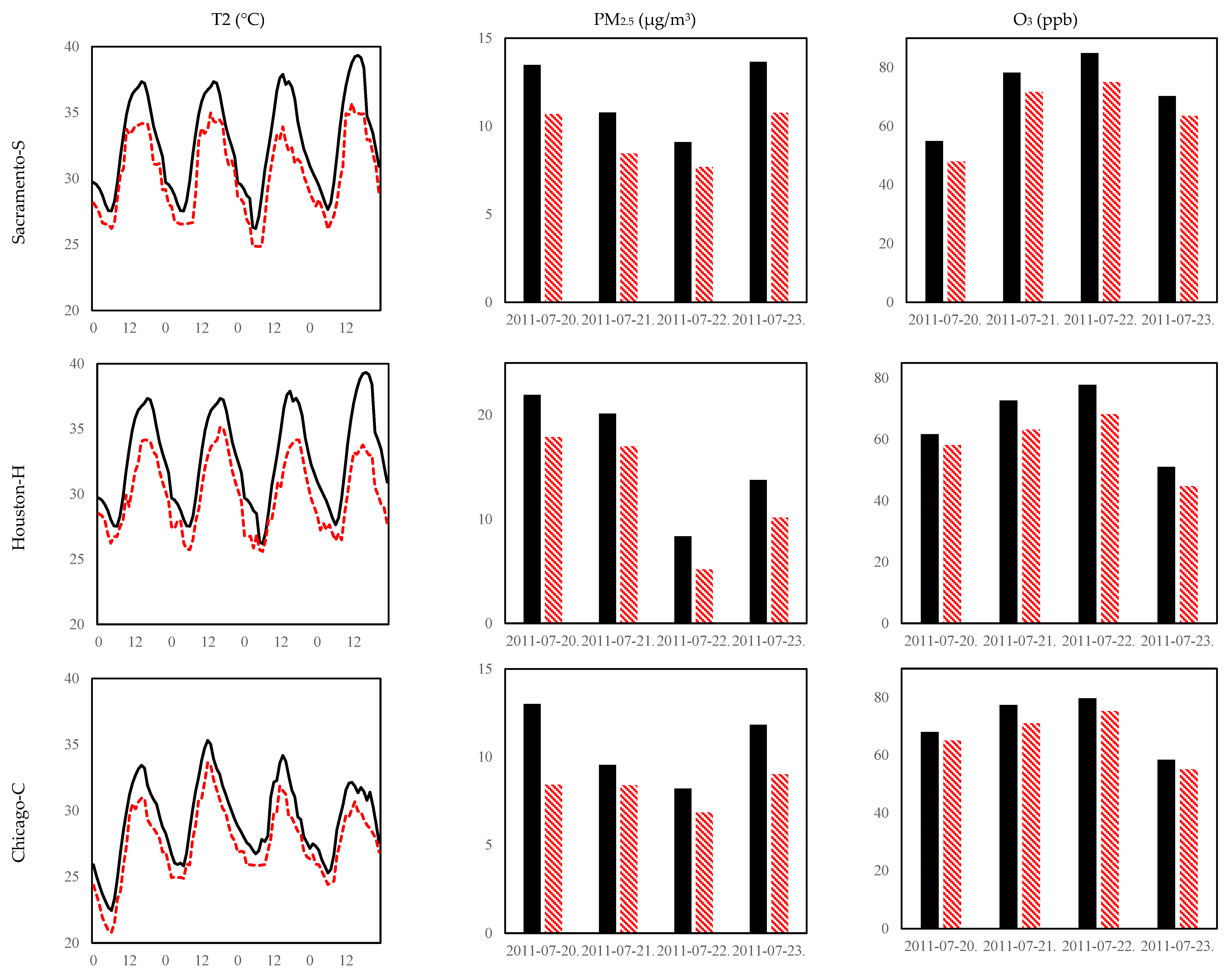
In terms of the chemical component of the model, the WRF_ChemV3.6.1, as configured here, tends to underpredict 24-h fine particular matters (PM2.5) and over-predict the 24-h O3 concentrations during the 2011 heat wave period. The MBE of the 24-h avg. PM2.5 is −1.42 µg/m3. The MAE and RMSE of PM2.5 are approximately 4 µg/m3. This is because the accuracy in fine particular matters concentrations is to some extent a function of its subspecies estimations as particulate sulfate, particulate nitrate, and organic carbons. Thus, we also compared the simulation results of SO42.5 (µg/m3), NO32.5 (µg/m3), and OC2.5 (µg/m3) with observations at urban areas of aforementioned cities. We observed that the performance of PM2.5 subspecies is a combination of overprediction of particulate sulfate (MBE ~ 5 µg/m3) and underprediction of particulate nitrate (MBE ~ −4 µg/m3) and organic carbon (MBE ~ −3 µg/m3). The MAE and RMSE of SO42.5, NO32.5, and OC2.5 are approximately 5, 4, and 3 µg/m3, respectively. The comparison between simulated ozone and measurements indicated an overestimation of O3 across the domains (MBE ~ 5 ppb). The O3 concentrations is overestimated due to the NOx and VOCs overestimation in emission inventories and their calculations in chemistry packages (US-NEI11 and MEGAN). The average MAE and RMSE of O3 are around 7 ppb and 8 ppb, respectively. We also calculated the NO2 concentrations as one of the precursor in ozone formation. The MBE of NO2 in urban areas (~2.5 ppb) show that the model tends to overpredict the nitrogen dioxide. The MAE and RMSE of NO2 is around 4 ppb.
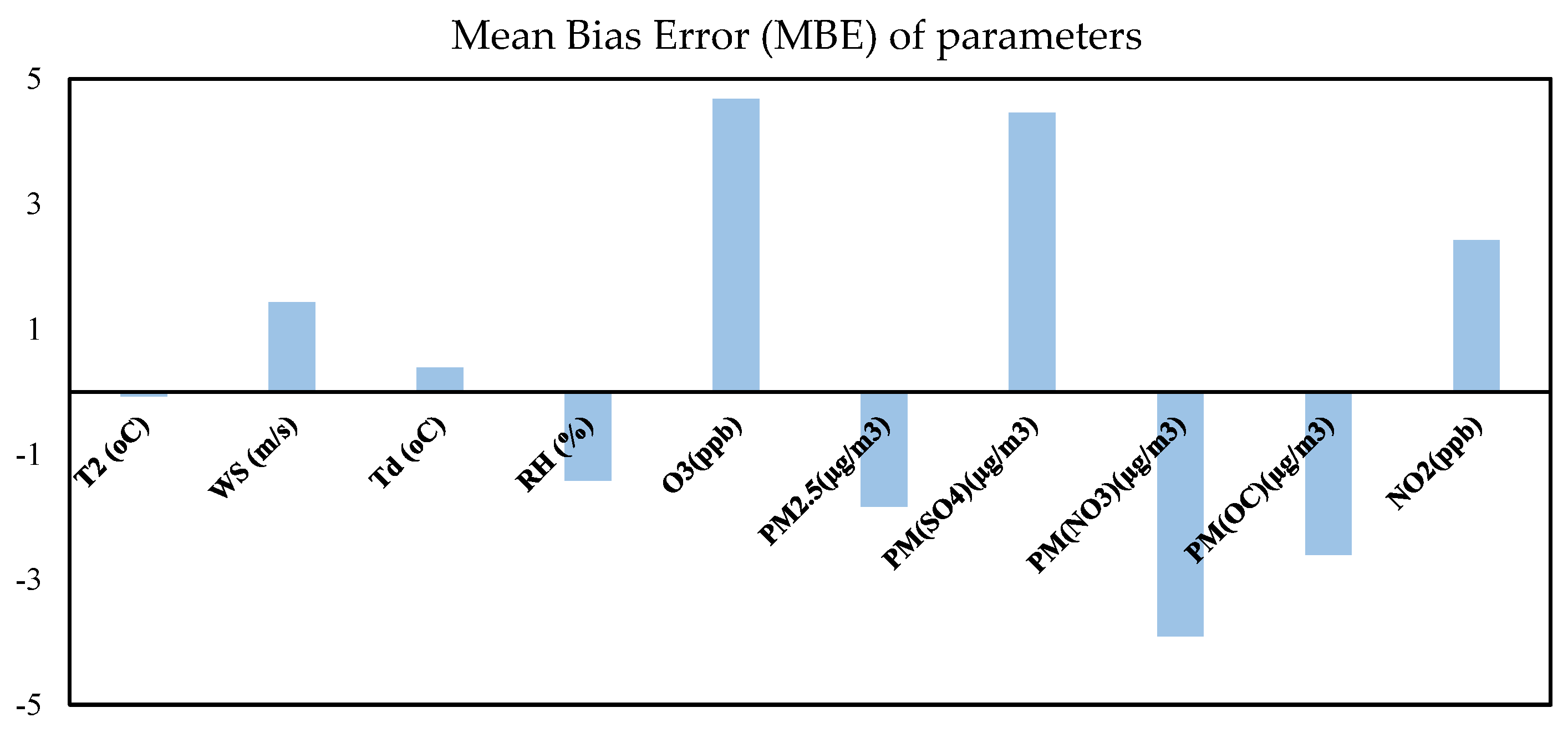
Figure 3 shows the observed vs. simulated PM2.5 (µg/m3) and O3 (ppb) concentrations in the urban areas of Sacramento, Houston, and Chicago. Table 3, Table 4 and Table 5 respectively represent the mean bias error (MBE), mean absolute error (MAE), and the root mean square error (RMSE) of T2 (°C), WS10 (m/s), RH2 (%), PM2.5 (µg/m3), and O3 (ppb) for aforementioned cities. There are several limitations and assumptions in these comparisons. The simulation results are extracted hourly for all variables, whereas the observation in terms of PM2.5 and O3 are reported as a 24-h average. Figure 4 shows the overall comparison between observed vs. simulated aforementioned parameters in terms of MBA, MAE, and RMSE. Despite the model biases in simulating meteorological and chemical variables, the performance of WRF-ChemV3.6.1 is generally consistent with most air quality models. For comparison of thermal components, the fifth-generation NCAR/Penn State Mesoscale Model (MM5) presented the MBE of T2 as 0.4 °C to −3.8 °C during a year [52,53,54,55]. For comparison of chemical components, the CMAQ model was run during a year and indicated an under estimation of PM2.5 as the MBE of −0.6 µg/m3 and an overprediction of seasonal O3 as the MBE of 4.4 ppb [56]. However, given the various differences in physical and chemical parameterizations and input data (different simulation year and observations), the online coupled WRF-Chem is mostly suited for application of simulating and investigating the effects of urban heat island and its mitigation strategies.
3.2. Effects of Increasing Urban Albedo
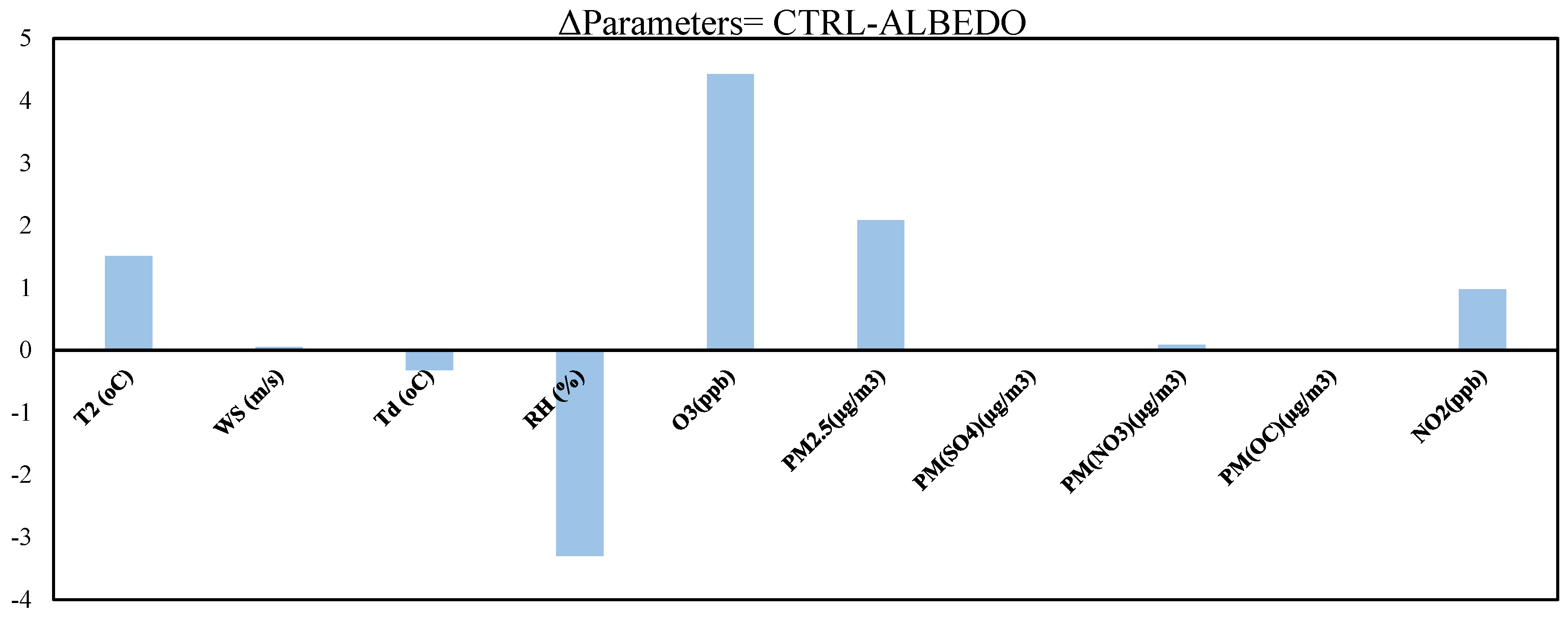
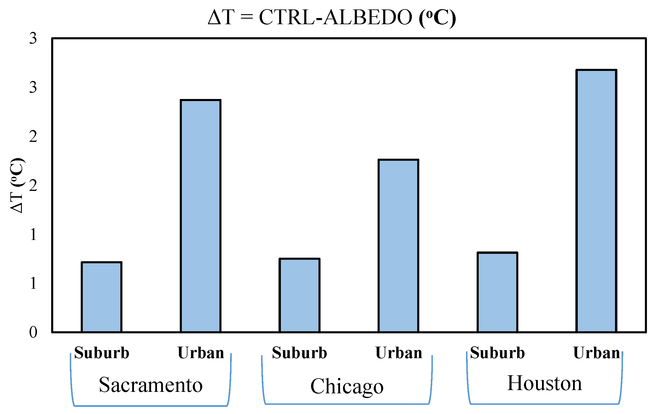
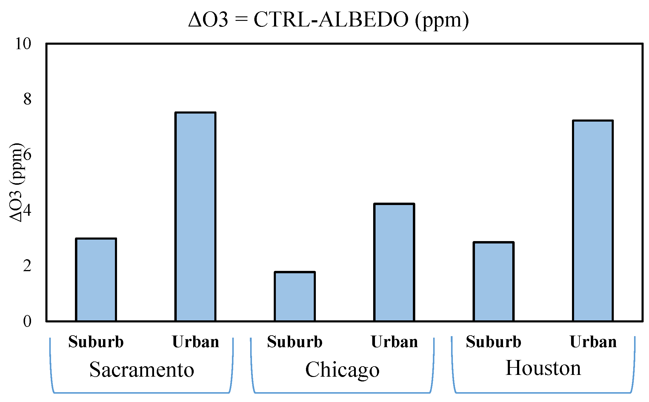
Results discussed here are based on the comparison between the ALBEDO and CTRL scenarios for each city. Table 6 and Figure 5 represent the average differences in T2 (°C), WS10 (m/s), Td (°C), RH2 (%), PM2.5 (µg/m3), O3 (ppb), SO42.5 (µg/m3), NO32.5 (µg/m3), OC2.5 (µg/m3), and NO2 (ppb) during the 2011 heat wave period across the second, third, and fourth domains: Sacramento (CA), Houston (TX), and Chicago (IL). Figure 6 shows the averaged differences of T2 (°C) and O3 (ppb) concentrations in suburb and urban areas of the aforementioned cities.
Sacramento, California is located in the central valley near the Sierra foothills. It is at the confluence of the Sacramento River and the American River and is known as the Sacramento Valley. The city has a population of approximately 500,000 people and covers over 253 km2 [57,58]. Its climate is characterized by mild year-round temperature. It has a hot-dry-summer Mediterranean climate with little humidity and an abundance of sunshine. Based on the National Oceanic and Atmospheric Administration (NOAA) Online Weather Data [22], Sacramento has the summer temperature exceeding 32 °C on 73 days and 38 °C on 15 days. The State of the Air 2017 report, by American Lung Association [59], ranks the metropolitan areas based on ozone and particular pollutions during 2013, 2014, and 2015 period. They used the official data from the U.S. Environmental Protection Agency (EPA). Sacramento ranks eighth because of its high ozone concentration.
In a study performed at the Lawrence Berkeley National Laboratory (LBNL), Taha et al. [60] applied the Colorado State Urban Meteorological Model (CSUMM) and the Urban Airshed Model (UAM-IV) to estimate the impacts of heat island mitigation strategies in Sacramento on the area’s local meteorology and ozone air quality in 2000. The albedo level and vegetative cover increased by approximately 0.11 and 0.14, respectively. Using 11–13 July 1990 as the modeling period, the ozone and temperature decreased by up to 10 ppb and 1.6 °C, respectively. In a more recent study, Taha et al. [61] applied WRF with CMAQ in Sacramento Valley with the inner domain of 1 km resolution. The albedo of roofs, walls, and pavements increased by 0.4, 0.1, and 0.2, respectively. The surface temperature and air temperature were reduced by up to 7 °C and 2–3 °C, respectively. The ozone concentrations also decreased by up to 5–11 ppb during the daytime.
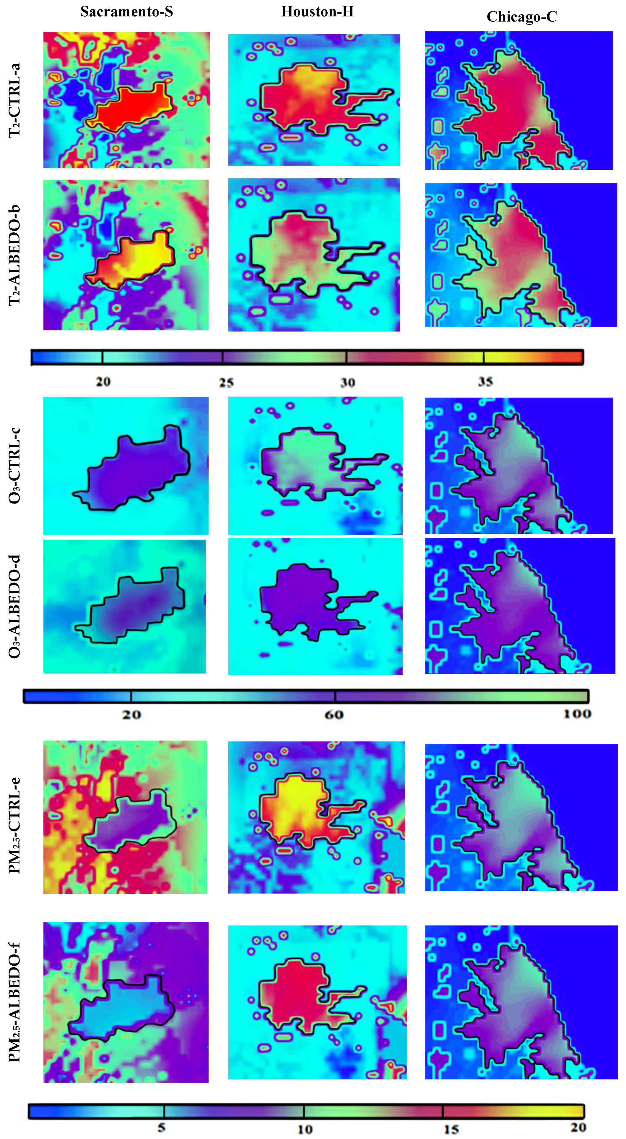
Our simulation results for Sacramento show that albedo enhancement leads to a net decrease in 2-m air temperature by up to 2.5 °C and 0.7 °C in urban and suburban areas, respectively. Most of the decreases occur between 1200 and 1600 LST as shown in Figure 7-S. Figure 8-Sa (CTRL) shows the maximum air temperature across the simulation domain in the heat wave period. By increasing surface reflectivity, the maximum temperature reduction is around 3 °C almost in all parts of the city (Figure 8-Sb-ALBEDO) and this reduction is more obvious in the western part of the domain. The wind speed slightly decreased over the entire domain. The relative humidity increased by 7% and 3% in urban and suburban areas, respectively. Increasing surface reflectivity affords a decrease of nearly 2.4 µg/m3 in PM2.5 concentrations in urban area (Figure 7-S) and 1 µg/m3 in suburb. Figure 8-Sc shows the maximum PM2.5 concentrations across the domain. The maximum is around 12 µg/m3 in urban area that decreases by 2–3 µg/m3 as the results of albedo enhancement (Figure 8-Sd). The heat island mitigation strategy causes a decline in O3 by almost 8 ppb in urban (Figure 7-S) and 3 ppb in suburb of the Sacramento area. Figure 8-Se shows the maximum O3 concentrations as nearly 80 ppb across the simulation domain that decreases to nearly 70 ppb by UHI mitigation strategy (Figure 8-Sf). Our results resemble those of previous studies [60,61,62,63]. We have also compared the CTRL and ALBEDO simulations results of particulate sulfate, particulate nitrate, organic carbon, and nitrogen dioxide. Albedo enhancement causes no changes (OC) to minimal changes to particular matters subspecies (~0.01 reduction) but decreases the NO2 concentration by 0.82 ppb.
Houston is the fourth most populous city in the U.S. with a population of 2.3 million within a land area of 1700 km2 [57,58]. It is located in the Southeast Texas near the Gulf of Mexico. Houston’s climate is classified as humid subtropical. During the summer, the temperature commonly reaches 34 °C, and some days it reaches to even 40 °C. The wind comes from the south and southeast and brings heat and moisture from the Gulf of Mexico. The highest temperature recorded in Houston is 43 °C, which occurred during the 2011 heat wave period [57,58]. Houston also suffers from excessive ozone levels and the American Lung Association [59] named the city as the 12th most polluted city in the U.S., based on EPA 2013, 2014, and 2015 data base.
Taha [64] used MM5 to evaluate the model’s episode performance and its response to increasing surface albedo and vegetation in Houston during several days in August 2000. In ALBEDO scenario, the roof albedo was increased from an average of 0.1 to an average of 0.3; wall albedo was increased from an average of 0.25 to an average of 0.3; pavement albedo was increased from an average of 0.08 to 0.2. The results indicated a reduction in temperature by up to 3.5 °C, and also caused warming in some areas by up to 1.5 °C. Results indicated that cooling usually occurs during daytime, while heating occurs at night. The other simulations show the same results [64,65,66].
Our simulation results for Houston show that albedo enhancement leads to a net decrease in 2-m air temperature by up to 3 °C and 0.8 °C in urban (Figure 7-H) and suburban areas, respectively. We witness no heating effect in our simulation. The reason is due to the sea breeze consideration in the solver of WRF-Chem. Figure 8-Ha illustrates the maximum air temperature across the Houston in the heat wave period. The maximum temperature reduction is above 3 °C almost in all parts of the city (Figure 8-Hb). Our model tends to perform relatively better in urban rather than in suburb areas. With albedo enhancement, the wind speed slightly decreased, and the relative humidity increased by up to 7% in urban and 3% in suburb. Increasing surface reflectivity affords a decrease of PM2.5 concentrations by up to 3.5 µg/m3 and 2.6 µg/m3 in urban and suburban areas, respectively. Figure 8-Hc shows the maximum PM2.5 concentrations across Houston. The maximum is above 20 µg/m3 in urban area that decreases to 16 µg/m3 as the results of albedo enhancement (Figure 8-Hd). The O3 concentrations also decrease by up to 7.2 ppb and 3 ppb in urban and suburban areas, respectively. Figure 8-He shows the maximum O3 concentrations as above 80 ppb across the simulation domain that decreases to nearly 70 ppb all over the domain (Figure 8-Hf). Our results resemble to previous studies [64,65,66]. Increasing surface albedo in the urban area of Houston causes no changes in particular matters subspecies and a decrease of 1.2 ppb in NO2 concentration.
Chicago is the third most populous city in the U.S. with over 2.7 million residents. The city area is 606 km2 [57,58]. The city lies on the southwestern shores of Lake Michigan and has two rivers: the Chicago River and the Calumet River. Chicago has a humid continental climate. Summer temperatures can reach up to 32 °C. Taha et al. [67] used a three-dimensional, Eulerian, mesoscale meteorological model (CSUMM) to simulate the effects of large scale surface modifications on meteorological conditions in 10 cities across the U.S. Surface modifications included increasing albedo by 0.03 ± 0.05 and increasing vegetative fraction by 0.03 ± 0.04. The results indicated that the air temperature was reduced by up to 1 °C in the Chicago area.
Our simulation results for Chicago show that albedo enhancement leads to a net decrease in 2-m air temperature by up to nearly 2 °C and 0.8 °C in urban (Figure 7-C) and suburban areas, respectively. Figure 8-Ca shows the maximum air temperature across the simulation domain. With albedo enhancement, the air temperature reduced over the domain (Figure 8-Cb). The wind speed slightly reduces in suburbs, with no changes in urban areas. The results show a slight decrease in relative humidity by up to 0.2% in Chicago’s urban areas. The reason is due to the wind speed direction that is north to west (passing the bodies of water) and the city’s location that is along one of the Great Lakes, Lake Michigan, and has the Mississippi River Watershed and the Chicago River. The other reason is due to the increasing surface reflectivity that reduces the skin temperature and thus air temperature that might also decrease the chance of evaporation and thus decreases moisture content above the ground. This strategy also affords a decrease of PM2.5 concentrations by up to 2.5 µg/m3 and 0.6 µg/m3 in urban and suburban areas, respectively. The maximum PM2.5 concentrations across Chicago is nearly 12 µg/m3, that decreases to nearly 9 µg/m3 as the results of albedo enhancement (Figure 8-Cc and Cd). The O3 concentrations decrease by up to 4.2 ppb in urban area and 1.7 ppb in suburb. Figure 8-Ce shows the maximum O3 concentrations as nearly 70 ppb across the simulation domain that decreases to almost 65 ppb all over the domain (Figure 8-Cf). Increasing urban albedo in Chicago leads to an increase of particulate nitrate by 3 ppb and a decrease of NO2 concentration by 0.9 ppb.
Overall, the results indicate that with albedo enhancement, the air temperature drops (~1.5 °C) and thus causes a decrease in ozone concentrations (~5 ppb) and nitrogen dioxide (~1 ppb). Increasing surface solar reflectance lead to a minimal decrease in particular matters (~2 µg/m3) and no significant changes in its subspecies. The SO42.5 and NO32.5 concentrations reduced slightly in urban areas (~0.1 µg/m3) due to the decrease in air temperature and thus photochemical reaction rates, but there is no change in OC2.5 (µg/m3). The UHI mitigation strategy increased the relative humidity and dew point temperature. Our results show that there are no significant changes in the wind speed over the domain and the differences between two scenarios is 0.05 m/s. This minimal change can be due to the WRF-Chem configurations and it does not reflect any changes in momentum transport from the shallow boundary layer.
4. Discussion
By comparing the simulation results with the observations, we acknowledge that WRF-Chem generally reproduces well the hourly variations of meteorological variables, but overpredicts or underpredicts the air pollutant concentrations during the 2011 heat wave period. One of the reasons is due to the method of comparison; the simulation outputs are extracted at the start of each hour, whereas the measurements are reported as hourly or daily averages. Another reason is because of the anthropogenic and the biogenic estimations by US-NEI11 (spatial resolution of 1 km) and MEGAN (spatial resolution of 4 km). The other issue is concerning the simulation episode which is seven consecutive days during the heat wave period, whereas the pollutants dispersion and formation may occur during a longer time period. We suggest a study to assess the effects of increasing surface albedo for a whole year to see its effects during the winter season and during a year as well. The WRF-Chem meteorological and chemical settings configured here are reasonable, but different settings may also be reasonable. We suggest alternative parameterizations to see the effects of surface albedo in a two-way nested approach such as ours for further studies. We also suggest assessing the effects of other UHI mitigation strategies (as increasing vegetative fraction) on urban climate and air quality within a two-way nested approach.
At the inception of our study, the WRF-Chem version 3.6.1 was the most recent release. Since our objectives are concerning the effects of urban heat island and its mitigation strategies on urban climate and there were no modifications in the multilayer of the urban canopy model, we decided to continue using this version. We run the model on 48 cores, 96 Gb for 14 days. Each actual day took 48 h to run on a supercomputer. The data assimilation in WRF can be used to update WRF model’s initial conditions. The WRF-DA is based on an incremental vibrational data assimilation technique and has both 3D-Var and 4D-Var capabilities. It also includes the capability of hybrid data assimilation (vibrational + ensemble). The conjugate gradient method is utilized to minimize the cost function in the analysis control variable space. Analysis increments are also interpolated to staggered grids and it gets added to the background (first guess) to get the final analysis of the WRF-model grid. The WRF has the capability to maintain data assimilation in its solver [29,30]. That is why our results show a good agreement with the observations. We believe our results and analyses are trustable and can be used for further investigations.
The 2011 heat wave period is selected for our simulations to investigate the effects of increasing albedo on the worst-case scenarios in each city. However, in order to specify the effects of increasing albedo, another simulation should be carried out in a normal condition during summer. Then the results need to be compared with the heat wave period to see the typical effects of albedo enhancement in each location. Simulation of the entire year can reveal more information on the annual effects of the mitigation strategy. To gain better results of the effectiveness of high-albedo strategy in improving the regional ozone air quality, other episodes and locations with more reliable emission inventories should be further investigated, modeled, and analyzed in a more detailed modeling approach. The information on an area’s local climate can help to focus on heat island mitigation strategies that best suit their region. For example, cities with dry climates may achieve greater benefits from increasing vegetative fraction of urban areas (more evapotranspiration) than would cities in humid climates. However, dry-climate cities also need to consider the availability of water to maintain vegetation. We suggest a more detailed analysis of simulation results to investigate the effects of surface modifications on decreasing the temperature-dependent photochemical reaction rates, as well as decreasing evaporation losses of organic compounds from industrial sectors, and mobile and stationary sources.
5. Summary and Conclusions
We applied a two-way nested approach in WRF-ChemV3.6.1 coupled with the ML-UCM to evaluate the surface modification consequences on air temperature, wind speed, relative humidity, dew point temperature, ozone, nitrogen dioxide, fine particulate matters, PM2.5 subspecies (particulate sulfate (SO42.5), particulate nitrate (NO32.5) and organic carbon (OC2.5)) concentrations in a unified continental scale through regional scales (North America through Sacramento, Houston, and Chicago) during the 2011 heat wave period. The two-way nested approach with fine-resolution modelling framework can equip us with an integrated simulation setup to capture the full impacts of meteorological and photochemical reactions. The applied method would serve as a basis for future model improvements and parameterization development, fine-resolution dispersion, and photochemical modelling for other geographical locations.
The model performance is evaluated by comparing the simulation results with the observations. Despite the model biases in simulating meteorological and chemical variables, the performance of WRF-ChemV3.6.1 is generally consistent with the most air quality models. [52,53,54,55,60,61,62,63,64,65,66,67], thus is mostly suited for application of simulating and investigating the effects of urban heat island and its mitigation strategies. The MBA, MAE, and RMSE estimations confirmed the model capabilities. For meteorological components, the WRF-ChemV3.6.1, as configured here, captures well the diurnal variations of 2-m air temperature (MBA ~ −0.07 °C), overpredicts 10-m wind speed (MBA ~ 1.65 m/s), overpredicts dew point temperature (MBA ~ 0.4 °C), underpredicts 2-m relative humidity (MBA ~ −1.4%). For chemical component, the model underpredicts the daily fine particular matters (PM2.5) (MBA ~ −1.5 µg/m3) and overpredicts the O3 concentrations (MBA ~ 5 ppb). The model underpredicts the NO2 (~2.5 ppb) and overpredicts particulate sulfate (MBE ~ 5 µg/m3) and underpredicts particulate nitrate (MBE ~ −4 µg/m3) and organic carbon (MBE ~ −3 µg/m3) in urban areas of aforementioned cities during the 2011 heat wave period. The model tends to perform relatively better in urban, rather than in suburban areas.
Two sets of simulations are conducted with regard to surface modifications: CTRL scenario and ALBEDO scenario. With albedo enhancement we observed: a decrease in air temperature by 2.3 °C in urban areas and 0.7 °C in suburban areas; a slight increase in wind speed; an increase in relative humidity (3%) and dew point temperature (0.3 °C); a decrease of PM2.5 and O3 concentrations by 2.7 µg/m3 and 6.3 ppb in urban areas and 1.4 µg/m3 and 2.5 ppb in suburban areas, respectively; minimal changes in PM2.5 subspecies and a decrease of nitrogen dioxide (1 ppb) in urban areas. The results presented here are episode- and region-specific and thus may not provide a suitable basis for generalization to other circumstances. Overall, the results confirm that for Sacramento in California, Houston in Texas, and Chicago in Illinois, the albedo enhancement is an effective mitigation strategy to reduce the air temperature and improve air quality. The results show that Sacramento and Houston benefit more from increasing surface solar reflectance. These findings are an asset for policy makers and urban planning designers. However, we suggest that the effects of other UHI mitigation strategies on urban climate and air quality should also be investigated before making decisions on applying any surface modifications. We also suggest running the simulations with more accurate emission inventories. We recommend a simulation for the entire year that can reveal more information of the mitigation strategy impacts.
Acknowledgments
Funding for this research was provided by the National Science and Engineering Research Council of Canada (NSERC) under Discovery Grants Program. Calcul Quebec and Compute Canada provided the computational facilities for this research.
Author Contributions
Zahra Jandaghian performed the simulations, analyzed the data and wrote the paper. Professor Hashem Akbari supervised the research, advised on the analyses, reviewed various drafts of the paper.
Conflicts of Interest
The authors declare no conflict of interest.
References
- Akbari, H.; Kolokotsa, D. Three decades of urban heat islands and mitigation technologies research. Energy Build. 2016, 133, 834–842. [Google Scholar] [CrossRef]
- Taha, H. Urban surface modification as a potential ozone air-quality improvement strategy in California: A mesoscale modeling study. Bound. Layer Meteorol. 2008, 127, 219–239. [Google Scholar] [CrossRef]
- Chen, F.; Yang, X.; Zhu, W. WRF simulations of urban heat island under hot-weather synoptic conditions: The case study of Hangzhou City, China. Atmos. Res. 2013, 138, 364–377. [Google Scholar] [CrossRef]
- Akbari, H.; Pomerantz, M.; Taha, H. Cool surfaces and shade trees to reduce energy use and improve air quality in urban areas. Sol. Energy 2001, 70, 295–310. [Google Scholar] [CrossRef]
- Salamanca, F.; Martilli, A. A numerical study of the Urban Heat Island over Madrid during the DESIREX (2008) campaign with WRF and an evaluation of simple mitigation strategies. Int. J. Climatol. 2012, 32, 2372–2386. [Google Scholar] [CrossRef]
- Fallmann, J.; Emeis, S.; Suppan, P. Mitigation of urban heat stress—A modelling case study for the area of Stuttgart. J. Geogr. Soc. Berl. 2013, 144, 202–216. [Google Scholar]
- Fallmann, J.; Forkel, R.; Emeis, S. Secondary effects of urban heat island mitigation measures on air quality. Atmos Environ. 2016, 125, 199–211. [Google Scholar]
- Touchaei, A.G.; Akbari, H.; Tessum, C.W. Effects of increasing urban albedo on meteorology and air quality Montreal (Canada)—Episodic simulation of heat wave in 2005. Atmos. Environ. 2016, 132, 188–206. [Google Scholar] [CrossRef]
- Jandaghian, Z.; Touchaei, G.A.; Akbari, H. Sensitivity analysis of physical parameterizations in WRF for urban climate simulations and heat island mitigation in Montreal. Urban Clim. 2017. [Google Scholar] [CrossRef]
- Seinfeld, J.H.; Pandis, S.N. Atmospheric Chemistry and Physics: From Air Pollution to Climate Change, 2nd ed.; John Wiley & Sons, Inc.: Hoboken, NJ, USA, 2012. [Google Scholar]
- Grell, G.A.; Peckham, S.E.; Schmitz, R.; McKeen, S.A.; Frost, G.; Skamarock, W.C.; Eder, B. Fully coupled “online” chemistry within the WRF model. Atmos. Environ. 2005, 39, 6957–6975. [Google Scholar] [CrossRef]
- Skamarock, W.C.; Klemp, J.B.; Dudhia, J.; Gill, D.O.; Barker, D.M.; Wang, W.; Powers, J.G. A Description of the Advanced Research WRF Version 3; National Center for Atmospheric Research: Boulder, CO, USA, 2008. [Google Scholar]
- Ahmadov, R.; McKeen, S.A.; Robinson, A.L.; Bahreini, R.; Middlebrook, A.M.; de Gouw, J.A.; Meagher, J.; Hsie, E.-Y.; Edgerton, E.; Shaw, S.; et al. A volatility basis set model for summertime secondary organic aerosols over the eastern United States in 2006. J. Geophys. Res. 2012, 117, 06–31. [Google Scholar] [CrossRef]
- Chuang, M.-T.; Zhang, Y.; Kang, D. Application of WRF/Chem-MADRID for real-time air quality forecasting over the southeastern United States. Atmos. Environ. 2011, 45, 6241–6250. [Google Scholar] [CrossRef]
- Misenis, C.; Zhang, Y. An examination of sensitivity of WRF/Chem predictions to physical parameterizations, horizontal grid spacing, and nesting options. Atmos. Res. 2010, 97, 315–334. [Google Scholar] [CrossRef]
- Zhang, Y.; Chen, Y.; Sarwar, G.; Schere, K. Impact of gas-phase mechanisms on Weather Research Forecasting Model with Chemistry (WRF/Chem) predictions: Mechanism implementation and comparative evaluation. J. Geophys. Res. 2012, 117, D01301. [Google Scholar] [CrossRef]
- Yahya, K.; Wang, K.; Gudoshava, M.; Glotfelty, T.; Zhang, Y. Application of WRF/Chem over North America under the AQMEII Phase 2: Part I. Comprehensive evaluation of 2006 simulation. Atmos. Environ. 2015, 155, 733–755. [Google Scholar] [CrossRef]
- Tessum, C.W.; Hill, J.D.; Marshall, J.D. Twelve-month, 12 km resolution North American WRF-Chem v3.4 air quality simulation: Performance evaluation. Geosci. Model. Dev. 2015, 8, 957–973. [Google Scholar] [CrossRef]
- Martilli, A.; Clappier, A.; Rotach, M. An urban surface exchange parameterization for mesoscale models. Bound. Layer Meteorol. 2002, 104, 261–304. [Google Scholar] [CrossRef]
- Liao, J.; Wang, T.; Wang, X.; Xie, M.; Jiang, Z.; Huang, X.; Zhu, J. Impacts of different urban canopy schemes in WRF/Chem on regional climate and air quality in Yangtze River Delta, China. Atmos. Res. 2014, 146, 226–243. [Google Scholar] [CrossRef]
- US-National Climate Data Centre (NOAA). Available online: https://www.ncdc.noaa.gov (accessed on 28 January 2018).
- NOAA. National Oceanic and Atmospheric Administration Changes to the NCEP Meso Eta Analysis and Forecast System: Increase in Resolution, New Cloud Microphysics, Modified Precipitation Assimilation, Modified 3DVAR Analysis. 2001. Available online: http://www.emc.ncep.noaa.gov/mmb/mmbpll/eta12tpb/ (accessed on 28 January 2018).
- Mesinger, F.; DiMego, G.; Kalnay, E.; Mitchell, K.; Shafran, P.C.; Ebisuzaki, W.; Jović, D.; Woollen, J.; Rogers, E.; Berbery, E.H.; et al. North American regional reanalysis. Bull. Am. Meteorol. Soc. 2006, 87, 343–360. [Google Scholar] [CrossRef]
- Lin, Y.; Farley, R.; Orville, H.D. Bulk parameterization of the snow field in a cloud model. J. Clim. Appl. Meteorol. 1983, 22, 1065–1092. [Google Scholar] [CrossRef]
- Chou, M.-D.; Suarez, M.J. A Solar Radiation Parameterization (CLIRAD-SW) Developed at Goddard Climate and Radiation Branch for Atmospheric Studies; NASA Technical Memorandum NASA/Goddard Space Flight Center Greenbelt: Greenbelt, MD, USA, 1999. [Google Scholar]
- Iacono, M.J.; Delamere, J.S.; Mlawer, E.J.; Shephard, M.W.; Clough, S.A.; Collins, W.D. Radiative forcing by longelived greenhouse gases: Calculations with the AER radiative transfer models. J. Geophys. Res. 2008, 113, 131–153. [Google Scholar] [CrossRef]
- Janjic, Z.I. The stepemountain Eta coordinate model: further developments of the convection, viscous sublayer, and turbulence closure schemes. Mon. Weather Rev. 1994, 122, 927–945. [Google Scholar] [CrossRef]
- Grell, G.A.; Devenyi, D. A generalized approach to parameterizing convection combining ensemble and data assimilation techniques. Geophys. Res. Lett. 2002, 29, 38–48. [Google Scholar] [CrossRef]
- NCAR. WRF User’s Guide; Mesoscale & Microscale Meteorology Division; National Center for Atmospheric Research (NCAR): Boulder, CO, USA, 2016. [Google Scholar]
- ARW User Guide. ARW Version 3 Modeling System User’s Guide; National Center for Atmospheric Research: Boulder, CO, USA, 2012. [Google Scholar]
- US EPA (US Environmental Protection Agency). 2011 National Emissions Inventory (NEI). Available online: http://www.epa.gov/ttn/ chief/emch/index.html (accessed on 7 March 2016).
- Guenther, A.B.; Jiang, X.; Heald, C.L.; Sakulyanontvittaya, T.; Duhl, T.; Emmons, L.K.; Wang, X. The Model of Emissions of Gases and Aerosols from Nature Version 2.1 (MEGAN2.1): An extended and updated framework for modeling biogenic emissions. Geosci. Model. Dev. 2012, 5, 1471–1492. [Google Scholar] [CrossRef] [Green Version]
- Ackermann, I.J.; Hass, H.; Memmesheimer, M.; Ebel, A.; Binkowski, F.S.; Shankar, U. Modal aerosol dynamics model for Europe: Development and first applications. Atmos. Environ. 1998, 32, 2981–2999. [Google Scholar] [CrossRef]
- Stockwell, W.R.; Kirchner, F.; Kuhn, M.; Seefeld, S. A new mechanism for regional atmospheric chemistry modeling. J. Geophys. Res. Atmos. 1997, 102, 25847–25879. [Google Scholar] [CrossRef]
- Schell, B.; Ackermann, I.J.; Hass, H.; Binkowski, F.S.; Ebel, A. Modeling the formation of secondary organic aerosol within a comprehensive air quality model system. J. Geophys. Res. Atmos. 2001, 106, 28275–28293. [Google Scholar] [CrossRef]
- Fast, J.D.; Gustafson, W.I., Jr.; Easter, R.C.; Zaveri, R.A.; Barnard, J.C.; Chapman, E.G.; Grell, G.A.; Peckham, S.E. Evolution of ozone, particulates, and aerosol direct radiative forcing in the vicinity of Houston using a fully coupled meteorology-chemistry-aerosol model. J. Geophys. Res. 2006, 111, 203–213. [Google Scholar] [CrossRef]
- Grell, G.A.; Freitas, S.R. A scale and aerosol aware stochastic convective parameterization for weather and air quality modeling. Atmos. Chem. Phys. 2014, 14, 5233–5250. [Google Scholar] [CrossRef]
- NCAR. WRF-CHEM Emission Guide; National Center for Atmospheric Research (NCAR) and The University Corporation for Atmospheric Research (UCAR): Boulder, CO, USA, 2016. [Google Scholar]
- NCAR. WRF-CHEM User’s Guide, WRF-Chem Emissions Guide; National Center for Atmospheric Research (NCAR): Boulder, CO, USA, 2016. [Google Scholar]
- Akbari, H.; Rose, L.S. Characterizing the Fabric of the Urban Environment: A Case Study of Metropolitan Chicago, Illinois; Report LBNL-49275; Lawrence Berkeley National Laboratory: Berkeley, CA, USA, 2001.
- Akbari, H.; Rose, L.S. Characterizing the Fabric of the Urban Environment: A Case Study of Salt Lake City, Utah; Report No. LBNL-47851; Lawrence Berkeley National Laboratory: Berkeley, CA, USA, 2001.
- Akbari, H.; Rose, L.S.; Taha, H. Analyzing the land cover of an urban environment using high-resolution orthophotos. Landsc. Urban Plan. 2003, 63, 1–14. [Google Scholar] [CrossRef]
- Rose, L.S.; Akbari, H.; Taha, H. Characterizing the Fabric of the Urban Environment: A Case Study of Greater Houston, Texas; Report LBNL-51448; Lawrence Berkeley National Laboratory: Berkeley, CA, USA, 2003.
- Millstein, D.; Menon, S. Regional climate consequences of large-scale cool roof and photovoltaic array deployment. Environ. Res. Lett. 2011, 6, 34–44. [Google Scholar] [CrossRef]
- EPA. 2005. Available online: http://www.epa.gov/ttnchie1/net/2005inventory.html (accessed on 28 January 2017).
- US EPA (Environmental Protection Agency). Technology Transfer Network (TTN) Air Quality System (AQS). 2005. Available online: http: //www.epa.gov/ttn/airs/airsaqs/detaildata/downloadaqsdata.htm (access on 6 March 2016).
- US EPA (US Environmental Protection Agency). Air Quality Modeling Technical Support Document for the Regulatory Impact Analysis for the Revisions to the National Ambient Air Quality Standards for Particulate Matter, Research Triangle Park, NC 27711. 2012. Available online: http://www.regulations.gov/ (accessed on 28 January 2018).
- UCAR (University Corporation for Atmospheric Research). GCIP NCEP Eta Model Output. 2005. Available online: http://rda.ucar.edu/ datasets/ds609.2/ (accessed on 15 January 2017).
- University of California Davis. IMPROVE Data Guide: A Guide to Interpret Data; Prepared for National Park Service, Air Quality Research Division: Fort Collins, CO, USA, 1995; Available online: http://vista.cira.colostate.edu/improve/publications/OtherDocs/IMPROVEDataGuide/IMPROVEdataguide.htm (accessed on 18 September 2017).
- Boylan, J.W.; Russell, A.G. PM and light extinction model performance metrics, goals, and criteria for three-dimensional air quality models. Atmos. Environ. 2006, 40, 4946–4959. [Google Scholar] [CrossRef]
- Zhang, Y.; Liu, P.; Pun, B.; Seigneur, C. A comprehensive performance evaluation of MM5-CMANQ for the summer 1999 southern oxidant study episode—Part I. Evaluation protocols, databases and meteorological predictions. Atmos. Environ. 2006, 40, 4825–4838. [Google Scholar] [CrossRef]
- Gilliam, R.C.; Hogrefe, C.; Rao, S.T. New methods for evaluating meteorological models used in air quality applications. Atmos. Environ. 2006, 40, 5073–5086. [Google Scholar] [CrossRef]
- Wu, S.-Y.; Krishnan, S.; Zhang, Y.; Aneja, V. Modelling atmospheric transport and fate of ammonia in North Carolina, part I. Evaluation of meteorological and chemical predictions. Atmos. Environ. 2008, 42, 3419–3436. [Google Scholar] [CrossRef]
- Wang, K.; Zhang, Y.; Jang, C.J.; Phillips, S.; Wang, B.-Y. Modelling study of Intercontinental air pollution transport over the Trans-Pacific region in 2001 using the community multiscale air quality (CMAQ) modelling system. J. Geophys. Res. 2009, 114, 4–19. [Google Scholar] [CrossRef]
- Liu, X.-H.; Zhang, Y.; Olsen, K.; Wang, W.-X.; Do, B.; Bridgers, G. Responses of future air quality to emission controls over North Carolina—Part I: Model evaluation for current-year simulations. Atmos. Environ. 2010, 44, 2443–2456. [Google Scholar] [CrossRef]
- Appel, K.W.; Chemel, C.; Roselle, S.J.; Francis, X.V.; Hu, R.-M.; Sokhi, R.S.; Rao, S.T.; Galmarini, S. Examination of the Community Multiscale Air Quality (CMAQ) model perfor-mance over the North American and European domains. Atmos. Environ. 2012, 53, 142–155. [Google Scholar] [CrossRef] [Green Version]
- US Census Bureau. Cartographic Boundary Shapefiles Regions. 2013. Available online: https://www.census.gov/geo/maps-data/data/cbf/cbf_region.html (accessed on 10 February 2017).
- US Census Bureau. Year-2014 US Urban Areas and Clusters. 2014. Available online: ftp://ftp2.census.gov/geo/tiger/TIGER2014/UAC/ (accessed on 10 February 2017).
- American Lung Association. 2017. Available online: http://www.lung.org/our-initiatives/healthy-air/sota/city-rankings/most-polluted-cities.html (accessed on 28 January 2018).
- Taha, H. Meso-urban meteorological and photochemical modeling of heat island mitigation. Atmos. Environ. 2008, 42, 8795–8809. [Google Scholar] [CrossRef]
- Taha, H.; Wilkinson, J.; Bornstein, R.; Xiao, Q.; McPherson, G.; Simpson, J.; Anderson, C.; Lau, S.; Lam, J.; Blain, C. An urban–forest control measure for ozone in the Sacramento, CA Federal Non-Attainment Area (SFNA). Sustain. Cities Soc. 2015, 21, 51–65. [Google Scholar] [CrossRef]
- Taha, H. Meteorological, emissions, and air-quality modeling of heat-island mitigation: Recent findings for California, USA. Int. J. Low Carbon Technol. 2013, 10, 3–14. [Google Scholar] [CrossRef]
- Taha, H. Ranking and Prioritizing the Deployment of Community-Scale Energy Measures Based on Their Indirect Effects in California’s Climate Zones. 2013. Available online: http://www.energy.ca.gov/2011publications/CEC-500-2011-FS/CEC-500-2011-FS-021.pdf (accessed on 28 January 2018).
- Taha, H. Potential Meteorological and Air-Quality Implications of Heat-Island Reduction Strategies in the Houston-Galveston TX Region; Technical Note HIG-12-2002-01; Lawrence Berkeley National Laboratory: Berkeley, CA, USA, 2003.
- Taha, H. Episodic Performance and Sensitivity of the Urbanized MM5 (uMM5) to Perturbations in Surface Properties in Houston Texas. Bound. Layer Meteorol. 2008, 127, 193–218. [Google Scholar] [CrossRef]
- Taha, H. Evaluating Meteorological Impacts of Urban Forest and Albedo Changes in the Houston-Galveston Region: A Fine-Resolution (UCP) Meso-Urban Modeling Study of the August–September 2000 Episode; Report Prepared for the Houston Advanced Research Center by Altostratus Inc.; Altostratus Inc.: Martinez, CA, USA, 2005. [Google Scholar]
- Taha, H.; Konopacki, S.; Gabersek, S. Impacts of Large-Scale Surface Modifications on Meteorological Conditions and Energy Use: A 10-Region Modeling Study. Theor. Appl. Climatol. 1999, 62, 175–185. [Google Scholar] [CrossRef]
Figure 1.
Simulation domains and land use/land cover over North America (mother domain) Sacramento, Houston, and Chicago (inner domains).
Figure 1.
Simulation domains and land use/land cover over North America (mother domain) Sacramento, Houston, and Chicago (inner domains).

Figure 2.
The time series (hourly) of the simulated (solid line) vs. measurements (dashed line) T2 (°C), WS10 (m/s), and RH2 (%) at urban monitoring stations across Sacramento, Houston, and Chicago.
Figure 2.
The time series (hourly) of the simulated (solid line) vs. measurements (dashed line) T2 (°C), WS10 (m/s), and RH2 (%) at urban monitoring stations across Sacramento, Houston, and Chicago.

Figure 3.
The time series (averaged 24-h) of simulated (black bar chart) vs. measurements (patterned downward diagonal bar chart) of PM2.5 (µg/m3) and O3 (ppb) concentrations at urban monitoring stations across Sacramento, Houston, and Chicago.
Figure 3.
The time series (averaged 24-h) of simulated (black bar chart) vs. measurements (patterned downward diagonal bar chart) of PM2.5 (µg/m3) and O3 (ppb) concentrations at urban monitoring stations across Sacramento, Houston, and Chicago.

Figure 4.
The overall mean bias error (MBE), mean absolute error (MAE), and root mean square error (RMSA) of T2 (°C), WS10 (m/s), Td (°C), RH2 (%), O3 (ppb), PM2.5 (µg/m3), SO42.5 (µg/m3), NO32.5 (µg/m3), OC2.5 (µg/m3), and NO2 (ppb) during the 2011 heat wave period.
Figure 4.
The overall mean bias error (MBE), mean absolute error (MAE), and root mean square error (RMSA) of T2 (°C), WS10 (m/s), Td (°C), RH2 (%), O3 (ppb), PM2.5 (µg/m3), SO42.5 (µg/m3), NO32.5 (µg/m3), OC2.5 (µg/m3), and NO2 (ppb) during the 2011 heat wave period.


Figure 5.
The average differences between CTRL and ALBEDO scenarios in T2 (°C), WS10 (m/s), RH2 (%), O3 (ppb), PM2.5 (µg/m3), SO42.5 (µg/m3), NO32.5 (µg/m3), OC2.5 (µg/m3), and NO2 (ppb) during the 2011 heat wave period.
Figure 5.
The average differences between CTRL and ALBEDO scenarios in T2 (°C), WS10 (m/s), RH2 (%), O3 (ppb), PM2.5 (µg/m3), SO42.5 (µg/m3), NO32.5 (µg/m3), OC2.5 (µg/m3), and NO2 (ppb) during the 2011 heat wave period.

Figure 6.
The average differences between CTRL and ALBEDO scenarios of T2 (°C) and O3 (ppb) during the 2011 heat wave period in suburb and urban areas of Sacramento, Chicago, and Houston.
Figure 6.
The average differences between CTRL and ALBEDO scenarios of T2 (°C) and O3 (ppb) during the 2011 heat wave period in suburb and urban areas of Sacramento, Chicago, and Houston.


Figure 7.
The differences between CTRL (solid line and black bar chart) and ALBEDO (red dashed line and patterned downward diagonal bar chart) scenarios in hourly T2 (°C) and 24-h avg. PM2.5 (µg/m3) and O3 (ppb) concentrations during the 2011 heat wave period across the urban areas of Sacramento-S, Houston-H, and Chicago-C.

Figure 8.
The maximum 2-m air temperature (°C), PM2.5 (µg/m3) and O3 (ppb) concentrations in CTRL and ALBEDO scenarios across Sacramento, Houston, and Chicago during the 2011 heat wave period.
Figure 8.
The maximum 2-m air temperature (°C), PM2.5 (µg/m3) and O3 (ppb) concentrations in CTRL and ALBEDO scenarios across Sacramento, Houston, and Chicago during the 2011 heat wave period.


Table 1.
Physical and chemical parameterizations in WRF_ChemV3.6.1.
| Category | Option Used |
|---|---|
| Microphysics | Lin scheme |
| Shortwave radiation | Goddard |
| Longwave radiation | RRTMG |
| Land surface model | NOAH |
| Planetary boundary layer scheme | Mellor–Yamada–Janjic Scheme |
| Cumulus parameterization | Grell Devenyi |
| Chemistry option | RACM |
| Photolysis scheme | Fast_J |
| Aerosol option | MADE/SORGAM |
| Advection scheme | Runge–Kutta third order |
| LULC data | USGS 24-class |
| Anthropogenic emissions | US-NEI11 |
| Biogenic emissions | MEGAN |
| Urban canopy model | ML-UCM |
Table 2.
Urban fabric of three cities in NA [43].
Table 2.
Urban fabric of three cities in NA [43].
| Metropolitan Areas | Roofs (%) | Pavements (%) |
|---|---|---|
| Sacramento | 20 | 45 |
| Chicago | 25 | 37 |
| Houston | 22 | 30 |
Table 3.
Mean bias error (MBE) of T2 (°C), WS10 (m/s), Td (°C), RH2 (%), O3 (ppb), PM2.5 (µg/m3), SO42.5 (µg/m3), NO32.5 (µg/m3), OC2.5 (µg/m3), and NO2 (ppb) at selected monitoring stations across Sacramento, Houston, and Chicago.
Table 3.
Mean bias error (MBE) of T2 (°C), WS10 (m/s), Td (°C), RH2 (%), O3 (ppb), PM2.5 (µg/m3), SO42.5 (µg/m3), NO32.5 (µg/m3), OC2.5 (µg/m3), and NO2 (ppb) at selected monitoring stations across Sacramento, Houston, and Chicago.
| Variables | Mean Bias Error (MBE) | Average | |||||
|---|---|---|---|---|---|---|---|
| Sacramento | Houston | Chicago | |||||
| Suburb | Urban | Suburb | Urban | Suburb | Urban | ||
| T2 (°C) | 0.15 | −0.34 | 0.22 | −0.34 | −0.30 | 0.19 | −0.07 |
| WS10 (m/s) | 1.90 | 3.15 | 0.87 | 0.34 | 1.28 | 1.05 | 1.43 |
| Td (°C) | 0.21 | 0.61 | 0.24 | 0.47 | 0.33 | 0.47 | 0.39 |
| RH2 (%) | −5.43 | −5.63 | −1.03 | 8.16 | 1.88 | −6.45 | −1.42 |
| 24-h avg. O3 (ppb) | 9.72 | 4.68 | 3.17 | 3.85 | 2.31 | 4.38 | 4.68 |
| 24-h avg. PM2.5 (µg/m3) | −5.94 | 2.30 | −3.26 | 2.07 | −3.86 | −2.33 | −1.84 |
| 24-h avg. SO42.5 (µg/m3) | - | 4.20 | - | 5.30 | - | 3.89 | 4.46 |
| 24-h avg. NO32.5 (µg/m3) | - | −3.75 | - | −4.40 | - | −3.52 | −3.91 |
| 24-h avg. OC2.5 (µg/m3) | - | −1.80 | - | −2.33 | - | −3.68 | −2.60 |
| 24-h avg. NO2 (ppb) | - | 2.61 | - | 3.40 | - | 1.25 | 2.42 |
Note: The definitions of statistical measurements are as follows Zhang et al. (2006) [51]: and are modeled and observed concentrations, respectively and N is the total number of model and observation pairs.
Table 4.
Mean absolute error (MAE) of T2 (°C), WS10 (m/s), Td (°C), RH2 (%), O3 (ppb), PM2.5 (µg/m3), SO42.5 (µg/m3), NO32.5 (µg/m3), OC2.5 (µg/m3), and NO2 (ppb) at selected monitoring stations across Sacramento, Houston, and Chicago.
Table 4.
Mean absolute error (MAE) of T2 (°C), WS10 (m/s), Td (°C), RH2 (%), O3 (ppb), PM2.5 (µg/m3), SO42.5 (µg/m3), NO32.5 (µg/m3), OC2.5 (µg/m3), and NO2 (ppb) at selected monitoring stations across Sacramento, Houston, and Chicago.
| Variables | Mean Absolute Error (MAE) | Average | |||||
|---|---|---|---|---|---|---|---|
| Sacramento | Houston | Chicago | |||||
| Suburb | Urban | Suburb | Urban | Suburb | Urban | ||
| T2 (°C) | 1.05 | 0.88 | 1.20 | 0.88 | 0.77 | 1.12 | 0.99 |
| WS10 (m/s) | 1.96 | 3.33 | 1.26 | 1.20 | 2.31 | 1.79 | 1.97 |
| Td (°C) | 0.56 | 0.30 | 0.49 | 0.63 | 0.56 | 0.66 | 0.53 |
| RH2 (%) | 15.32 | 9.45 | 5.38 | 9.54 | 8.98 | 10.11 | 9.80 |
| 24-h avg. O3 (ppb) | 9.72 | 9.90 | 6.92 | 6.01 | 2.56 | 5.88 | 6.83 |
| 24-h avg. PM2.5 (µg/m3) | 6.24 | 3.05 | 3.26 | 3.70 | 3.86 | 2.33 | 3.74 |
| 24-h avg. SO42.5 (µg/m3) | - | 4.20 | - | 5.30 | - | 3.89 | 4.46 |
| 24-h avg. NO32.5 (µg/m3) | - | 3.75 | - | 4.45 | - | 3.52 | 3.91 |
| 24-h avg. OC2.5 (µg/m3) | - | 1.80 | - | 2.33 | - | 3.68 | 2.60 |
| 24-h avg. NO2 (ppb) | - | 4.71 | - | 3.40 | - | 2.54 | 3.55 |
Note: The definitions of statistical measurements are as follows Zhang et al. (2006) [51]: and are modeled and observed concentrations, respectively and N is the total number of model and observation pairs.
Table 5.
Root mean square error (RMSE) of T2 (°C), WS10 (m/s), Td (°C), RH2 (%), O3 (ppb), PM2.5 (µg/m3), SO42.5 (µg/m3), NO32.5 (µg/m3), OC2.5 (µg/m3), and NO2 (ppb) at selected monitoring stations across Sacramento, Houston, and Chicago.
Table 5.
Root mean square error (RMSE) of T2 (°C), WS10 (m/s), Td (°C), RH2 (%), O3 (ppb), PM2.5 (µg/m3), SO42.5 (µg/m3), NO32.5 (µg/m3), OC2.5 (µg/m3), and NO2 (ppb) at selected monitoring stations across Sacramento, Houston, and Chicago.
| Variables | Root Mean Square Error (RMSE) | Average | |||||
|---|---|---|---|---|---|---|---|
| Sacramento | Houston | Chicago | |||||
| Suburb | Urban | Suburb | Urban | Suburb | Urban | ||
| T2 (°C) | 1.35 | 1.13 | 1.44 | 1.13 | 1.01 | 1.32 | 1.23 |
| WS10 (m/s) | 2.29 | 3.68 | 1.58 | 1.47 | 2.86 | 2.22 | 2.35 |
| Td (°C) | 0.68 | 0.37 | 0.58 | 0.77 | 0.67 | 0.80 | 0.65 |
| RH2 (%) | 18.94 | 12.32 | 7.52 | 12.26 | 11.36 | 13.48 | 12.65 |
| 24-h avg. O3 (ppb) | 10.51 | 14.21 | 7.89 | 6.71 | 3.09 | 8.21 | 8.44 |
| 24-h avg. PM2.5 (µg/m3) | 7.74 | 3.25 | 4.04 | 4.30 | 4.82 | 2.81 | 4.49 |
| 24-h avg. SO42.5 (µg/m3) | - | 4.44 | - | 6.24 | - | 3.93 | 4.87 |
| 24-h avg. NO32.5 (µg/m3) | - | 3.96 | - | 4.87 | - | 4.28 | 4.37 |
| 24-h avg. OC2.5 (µg/m3) | - | 1.93 | - | 2.39 | - | 3.76 | 2.69 |
| 24-h avg. NO2 (ppb) | - | 5.74 | - | 4.10 | - | 2.89 | 4.24 |
Note: The definitions of statistical measurements are as follows Zhang et al. (2006) [51]: and are modeled and observed concentrations, respectively and N is the total number of model and observation pairs.
Table 6.
The differences between CTRL and ALBEDO scenarios of T2 (°C), WS10 (m/s), RH2 (%), O3 (ppb), PM2.5 (µg/m3), SO42.5 (µg/m3), NO32.5 (µg/m3), OC2.5 (µg/m3), and NO2 (ppb) during the 2011 heat wave period across Sacramento, Houston, and Chicago.
Table 6.
The differences between CTRL and ALBEDO scenarios of T2 (°C), WS10 (m/s), RH2 (%), O3 (ppb), PM2.5 (µg/m3), SO42.5 (µg/m3), NO32.5 (µg/m3), OC2.5 (µg/m3), and NO2 (ppb) during the 2011 heat wave period across Sacramento, Houston, and Chicago.
| Δ ALBEDO | |||||||
|---|---|---|---|---|---|---|---|
| CTRL-ALBEDO | Sacramento | Houston | Chicago | Average | |||
| Suburb | Urban | Suburb | Urban | Suburb | Urban | ||
| Δ T2 (°C) | 0.72 | 2.37 | 0.81 | 2.68 | 0.75 | 1.76 | 1.52 |
| Δ WS10 (m/s) | 0.03 | 0.02 | 0.33 | 0.02 | −0.08 | 0.00 | 0.05 |
| Δ Td (°C) | −0.26 | −0.39 | −0.27 | −0.46 | −0.21 | −0.34 | −0.32 |
| Δ RH2 (%) | −2.99 | −6.88 | −2.44 | −6.89 | −0.81 | 0.21 | −3.30 |
| 24-h avg. O3 (ppb) | 2.98 | 7.52 | 2.85 | 7.23 | 1.77 | 4.23 | 4.43 |
| 24-h avg. PM2.5 (µg/m3) | 0.98 | 2.36 | 2.59 | 3.49 | 0.61 | 2.48 | 2.08 |
| 24-h avg. SO42.5 (µg/m3) | - | 0.02 | - | 0.01 | - | 0.06 | 0.03 |
| 24-h avg. NO32.5 (µg/m3) | - | 0.01 | - | 0.05 | - | 0.23 | 0.09 |
| 24-h avg. OC2.5 (µg/m3) | - | 0.00 | - | 0.00 | - | 0.00 | 0.00 |
| 24-h avg. NO2 (ppb) | - | 0.82 | - | 1.21 | - | 0.91 | 0.98 |
© 2018 by the authors. Licensee MDPI, Basel, Switzerland. This article is an open access article distributed under the terms and conditions of the Creative Commons Attribution (CC BY) license (http://creativecommons.org/licenses/by/4.0/).
Share and Cite
MDPI and ACS Style
Jandaghian, Z.; Akbari, H. The Effect of Increasing Surface Albedo on Urban Climate and Air Quality: A Detailed Study for Sacramento, Houston, and Chicago. Climate 2018, 6, 19. https://0-doi-org.brum.beds.ac.uk/10.3390/cli6020019
AMA Style
Jandaghian Z, Akbari H. The Effect of Increasing Surface Albedo on Urban Climate and Air Quality: A Detailed Study for Sacramento, Houston, and Chicago. Climate. 2018; 6(2):19. https://0-doi-org.brum.beds.ac.uk/10.3390/cli6020019
Chicago/Turabian StyleJandaghian, Zahra, and Hashem Akbari. 2018. "The Effect of Increasing Surface Albedo on Urban Climate and Air Quality: A Detailed Study for Sacramento, Houston, and Chicago" Climate 6, no. 2: 19. https://0-doi-org.brum.beds.ac.uk/10.3390/cli6020019
Note that from the first issue of 2016, this journal uses article numbers instead of page numbers. See further details here.