The Effect of Building Facades on Outdoor Microclimate—Reflectance Recovery from Terrestrial Multispectral Images Using a Robust Empirical Line Method

Abstract

Climate change and the urban heat island effect pose significant health, energy and economic risks. Urban heat mitigation research promotes the use of reflective surfaces to counteract the negative effects of extreme heat. Surface reflectance is a key parameter for understanding, modeling and modifying the urban surface energy balance to cool cities and improve outdoor thermal comfort. The majority of urban surface studies address the impacts of horizontal surface properties at the material and precinct scales. However, there is a gap in research focusing on individual building facades. This paper analyses the results of a novel application of the empirical line method to calibrate a terrestrial low-cost multispectral sensor to recover spectral reflectance from urban vertical surfaces. The high correlation between measured and predicted mean reflectance values per waveband (0.940 (Red) < r_s > 0.967 (NIR)) confirmed a near-perfect positive agreement between pairs of samples of ranked scores. The measured and predicted distributions exhibited no statistically significant difference at the 95% confidence level. Accuracy measures indicate absolute errors within previously reported limits and support the utility of a single-target spectral reflectance recovery method for urban heat mitigation studies focusing on individual building facades.

1. Introduction

Anthropogenic alterations to the optical, thermal, moisture and aerodynamic properties of city surfaces generate distinct urban climates, typically characterized by the urban heat island (UHI) effect [1]. The UHI effect refers to hotter air (and surface) temperatures observed in cities compared to non-urban surroundings [2]. UHI spatial and temporal characteristics are influenced by synoptic weather conditions [3,4] but UHI formation is attributed to differences in urban surface structure (3-D geometry), cover (land use and permeability), fabric (optical and thermal properties of materials) and metabolism (human activity) compared to non-urban surroundings [5,6]. Geometric and surface characteristics regulate the partitioning of the surface energy balance (SEB) [2] and at any given location surface temperature—and near-surface air temperature under calm conditions [7,8]—is controlled by the surface’s SEB [9].

UHIs develop in most cities regardless of climate [10] and have been observed globally in over 400 urban areas [4]. The magnitude of the screen height air temperature difference between urban and non-urban locations, or between different Local Climate Zones [10], is quantified by the “UHI intensity” which is most pronounced during calm, clear summer nights [2]. The average maximum UHI intensity for 87 European cities has been reported to be almost 6.2 K within a range of 2.8 K to 12 K [11]. Similar magnitude UHI intensities were reported for 101 Asian and Australian cities [12].

The superimposition of inadvertent urban heating (i.e., UHIs) and global warming, including more frequent, longer and intense heat waves [13,14,15] elevates the risk of heat-related mortality and illness in cities [16,17,18] and extreme urban heat has detrimental outdoor comfort, economic and building energy impacts [19,20,21]. The intentional modification of urban surface geometry, cover and fabric to reduce urban heat and decouple heat waves from amplified UHIs [22,23] is now a policy priority for many cities [24,25].

1.1. Urban Heat Mitigation—Current Status and Cooling Magnitude

In summer, solar absorption by urban surfaces is the dominant cause of the UHI effect [5]. Recent efforts to mitigate the formation of urban heat at different spatial scales have focused on changes to urban surface geometry and fabric [26,27,28] with the primary aim of controlling the absorption of solar radiation and increasing moisture availability [22,29]. However, due to the significant urban surface and air temperature reduction potential of reflective technologies [19,30] heat mitigation solely focusing on “cool” materials—those with high solar reflectance and high infrared emittance [31,32,33]—applied to building envelopes (roofs and walls) and urban structures (roads, squares and footpaths) dominates current scientific research and the global implementation of UHI mitigation technologies [34].

An analysis of 75 simulation studies using reflective materials on roofs and pavements reported average peak and absolute maximum screen-height air temperature reductions of 1.43 K and 3.4 K respectively for their combinations [35]. The same study reported average reductions in air temperature of 0.23 K and 0.27 K per 10% increase in albedo for cool roofs and cool pavement technologies respectively. However, despite widespread acceptance of the cooling benefits of reflective technologies and the implementation of numerous large-scale projects using reflective roof and pavement materials [36], more rigorous experimental monitoring, consistent metadata reporting and detailed information on their reduced performance over time and potential outdoor comfort impacts are still required [37,38,39].

1.2. Urban Heat Mitigation—Principles of Reflective Technology

The primary summer daytime energy input into the urban canopy layer (UCL) is solar radiation, which is reflected or absorbed by solar-exposed terrestrial surfaces [1]. Depending on surface characteristics, solar radiation is partitioned into radiative, sensible, latent or storage heat fluxes [2,40,41]. Radiative and sensible heat fluxes dominate the SEB in the absence of moisture [42,43]. Sensible heat—or the perceptible rise in air temperature—is amplified when the difference between surface and ambient temperatures is large [44,45]. A reduction in the surface’s surface temperature, which is achieved by shade or increasing the surface’s reflectance [46,47] constrains the convective transfer intensity to the surrounding air [44], thus limiting the transfer of heat to the adjacent air volume [42,43,48] although the relationship between surface and near-surface air temperature is complex [49].

Conversely, surfaces with lower solar reflectance absorb more solar energy, thereby heating the surface, and through strengthened convective transfer [45], warm the adjacent air volume [46,50]. Additionally, via long-wave radiative transfer, hotter surfaces emit infrared radiation to cooler objects within view [51]. In summary, increasing surface reflectance—which in the solar spectrum is referred to as the surface’s albedo—potentially reduces the surface’s surface temperature, the convective transfer intensity to the air and the emitted infrared radiation to surfaces in view.

However, higher solar reflectance within cities may also increase reflected solar radiation to near-surface facets and people [37,51,52,53,54,55,56,57,58,59] although the magnitude of reflected solar radiation and its impact on human outdoor thermal comfort is highly context-dependent [37,53,60] and few studies have been experimentally determined [52,54].

1.3. Methods for Measuring Solar Reflectance—Nomenclature

The albedo of a surface is defined as its hemispherical and wavelength-integrated reflectance [50] and broadband albedo is the ratio of reflected to incident (direct and diffuse) solar radiation (250–3000 nm), or the fraction of incident sunlight reflected by the surface quantified from 0 to 1 [61]. The albedo of a terrestrial surface may vary with the wavelength (λ) of incident radiation (spectral dependence), the angle of incidence (θ) of radiation (angular dependence of direct and diffuse components) and the surface’s surface structure and roughness [61,62].

In remote sensing and field measurements reflectance quantities are acquired under sky conditions and surface albedo is influenced by atmospheric turbidity, solar position, surface orientation and the geometry and optical properties of the surrounding urban form [62,63]. Solar irradiance consists of both direct beam and diffuse components and therefore the solar reflectance of a surface is variable in time and place (as atmospheric conditions and solar position change) and constant albedo values assume spectral and angular independence [62].

The use of laboratory, field or remote sensing methods for the measurement of surface reflectance is determined by the experimental design, material characteristics (e.g., sample size, etc.), spatial scale and wavelength and directional parameters of interest [64,65,66]. Reflectance nomenclature describes measured reflectance values first by the incident, and secondly by the reflected, angular distribution of radiation [63]. Levinson et al. [66] provide a comprehensive review of standard reflectance measurement methods and only remotely-sensed reflectance methods are briefly discussed further here.

1.4. Methods for Measuring Solar Reflectance—Remote Sensing of Urban Surfaces Using Narrow Field of View (FOV) Sensors

The standards-based laboratory [67] and field methods [68,69] for albedo measurement provide single reflectance quantities of small (0.1–5 cm²), flat, homogenous surfaces or the hemispherically-integrated value of larger (>1 m²) horizontal and low-sloped homogeneous diffusely-reflecting surfaces or the aggregate quantity of non-uniform horizontal surfaces [70] with relatively high accuracy (error <2%) [66]. However, the aforementioned methods have several limitations when applied to real urban surfaces [64,66,71,72].

Since the microclimate impacts of urban vertical surfaces are spatially dependent [54,73,74,75,76] and may be significantly influenced by microstructure heterogeneity [77] the ability to compute the spatial and geometric distribution of reflectance at sub-facet scale (<10 m) is desirable [78,79,80,81,82]. Satellite, aerial and ground-based remote sensing technologies permit increasing spatial, spectral, radiometric and temporal resolution with greater spatial coverage [48,83,84]. Ground-based imaging sensors are lightweight and mobile enabling in-canyon observations of surfaces with relative operational simplicity [85].

Remote sensors record wavelength-dependent energy emanating from a surface within the sensor’s FOV. At short path lengths near the ground (<100–200 m) atmospheric absorption may be considered to be negligible [84,86,87]. Image data from image sensors are composed of discrete picture elements (pixels) each with a potentially unique brightness (or digital number, DN) value and ground resolution or instantaneous field of view (IFOV) determined by the sensor optics [84]. Depending on target distance, a ground-based image of a building wall or horizontal urban surface is “automatically” resolved into sub-facet (IFOV) scale surface brightness values that, once calibrated to spectral radiance [63] and geolocated, can be used to derive spatially-registered per-pixel spectral reflectance quantities based on the experimentally determined correlation between surface reflectance and at-sensor radiance [48,88,89].

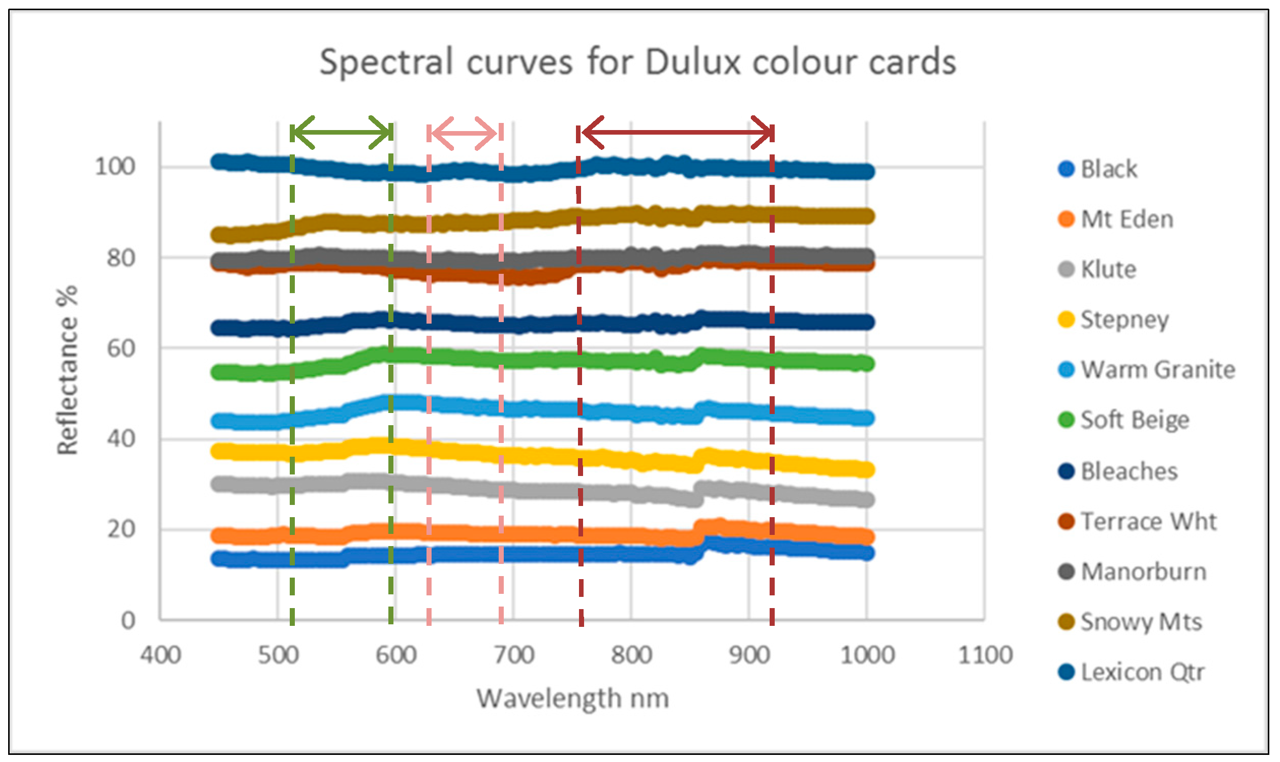
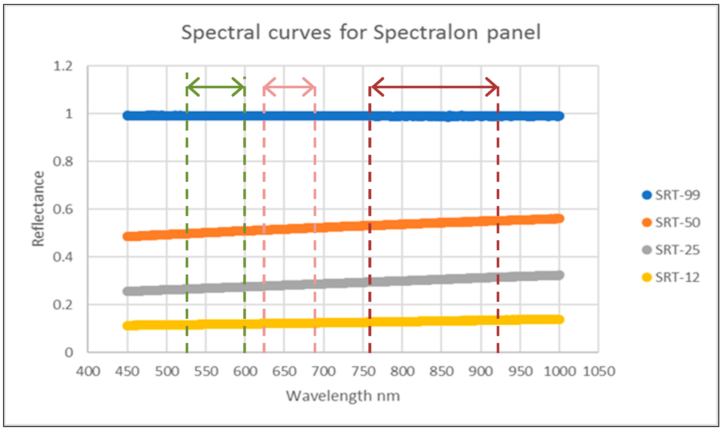
Obtaining reflectance data in both the visible and NIR wavelengths improves surface albedo estimates, since many urban materials strongly reflect in the NIR region [31,48,90]. Multispectral (MS) sensors are spectrally selective and simultaneously record reflected radiation in several discrete narrow bandwidths, for example in Green (520–600 nm), Red (630–690 nm) and NIR (760–920 nm) [91,92]. Reflectance quantities derived from ground-based sensors with narrow FOV (and with knowledge of the surfaces’ spectral and angular dependence [48]) are “hemispherical-canonical” reflectance values (per [63]) where direct and diffuse sky radiation is reflected into a narrow sensor viewing geometry [63]. A maximum absolute error of 14% has been reported for remotely measured albedo values of horizontal and low-sloped urban roofs from radiometrically calibrated high-resolution (1 m) aerial imagery with a smaller error (<2%) for low albedo (<0.2) surfaces [48].

1.5. Methods for Measuring Solar Reflectance—Overview of the Emprical Line (EL) Method

Remotely sensed image data of reflected energy received by a passive sensor is typically represented by a matrix of pixels containing DNs that are in value proportional to the intensity of energy reflected by the surface within view [92]. However, the proportionality relationship between image DNs and physical units such as surface reflectance is influenced by camera characteristics (i.e., the spectral response curve and analogue-to-digital signal conversion of the sensor [92]), sun-surface-sensor geometry (i.e., anisotropy of reflected radiation and illumination conditions [93]) and, for larger path distances, atmospheric transmittance [48]. Hence, DNs alone contain little meaningful quantitative information about surface reflectance unless the sensor is radiometrically calibrated [88].

Empirical (or “vicarious”) radiometric calibration using in-situ reference targets of known spectral reflectance correlated to at-sensor radiance for each sensor waveband robustly accounts for atmospheric and illumination effects and produces acceptable radiance-to-reflectance conversion results [48,88]. Despite its widespread use the method is error prone if implemented without logistical and methodological considerations [88,94]. For many inexpensive, commercially available MS cameras the relationship between at-sensor spectral radiance and image DNs is not readily available [95,96], is onerous to obtain [48,97] and may be non-linear [98] and the unique camera response function—the gain and offset coefficients used to convert the radiance-as-electrical signal to output digital numbers [92]—requires determination before DNs can be converted to reflectance units [99,100]. In this case, the reflectance-based calibration method can be used to predict at-sensor radiance (expressed as image DNs) by measuring the reflectance of a calibration target [94,100].

Typically, an ordinary least squares (OLS) regression equation of spectral reflectance (y-axis) against DNs (x-axis) is computed for each sensor waveband from the mean spectral reflectance values of at least two spectrally distinct ground calibration targets and the mean DNs from the corresponding region of interest (ROI) in the image [88]. The EL equation is then validated in the field using spectral reflectance values measured by a field spectrometer or supplementary targets of known reflectance [86,99]. Mean DNs retrieved from remotely sensed MS images are then used as input data to the per-waveband predictive equations to generate per-pixel spectral reflectance values [86,96,101,102]. Several authors have developed simplified protocols using vicarious calibration methods to reduce the number of high-cost, in-situ and in-image targets [86,98].

While studies using EL methods for reflectance recovery are increasingly common to derive vegetation characteristics in open fields ([86] and references therein) the use of the EL method for reflectance recovery from urban surfaces is less common due to logistical and methodological challenges posed by urban areas [5] but interest in applications to man-made and urban surfaces is growing [94,103,104].

1.6. Purpose and Significance of the Work

Surface properties and impacts of cool roof and paving technologies have been extensively studied and applied [19,26,32,36,46,105,106,107]. However, research into the microclimate impacts of urban vertical surfaces and the effect of building facade geometry and fabric remain relatively underdeveloped [44]. While research into the optical properties, thermal and energy performance and outdoor thermal comfort impacts of cool materials for use in building envelopes is more advanced [36,37,54,72,73,108,109,110,111,112,113], the conceptualisation of building facades as more than merely an ensemble of material “facets” (or discrete, homogenous, surfaces [5]) and the development of climate sensitive architectural design applications that progress beyond a singular focus on cool and smart material specification [114,115,116] are still emerging (e.g., [117,118,119,120]).

While microclimate modelling and simulation tools exist and are fundamentally useful [121,122,123] comparatively few have been validated in the field [124] and none explicitly provide architects with meaningful “thermo-semantics”—the synthesis of building envelope thermal and optical performance computation and architectural design—at scales and interests commensurate with architects’ decision-making [125].

This paper is part of ongoing research into the development of a thermo-semantic tool intended to assist architects to evaluate the outdoor thermal impacts of building facade design based on a vertical surface thermal typology supported by a predictive statistical model. The reflectance recovery method described here was applied to multispectral image panoramas of sampled building facades to create reflectance datasets for input to a probabilistic model.

The development of low-cost, replicable methods for reflectance recovery from real urban vertical surfaces within the UCL addresses the need for improved observation, understanding and transdisciplinary communication of urban atmospheric process at multiple scales and particularly at the street-level human scale [126] and contributes to the development of a predictive science of microclimatology [125]. Close-range ground-based reflectance recovery complements but also has some advantages over emerging unmanned aerial vehicle (UAV) technologies, particularly in relation to the statutory height and air-space restrictions applicable to UAVs in dense urban areas [86,127].

2. Materials and Methods

2.1. Overview of Method

To recover per-pixel spectral reflectance from MS digital images the relationship between known reflectance values per camera waveband and image DN distributions was statistically modelled as EL equations [88]. Two sets of alternative camera calibration targets were used to derive the theoretical constant “camera response function” and a second calibration target of higher reflectance was used to derive the variable “slope coefficient” [98]. The reflectance recovery method was evaluated by comparing known reflectance values of common building materials used in building facades with those derived from the final empirical line equations applied in ArcMap (ArcGIS by ESRI) to colour-processed MS images of the same materials. Predictive model precision and accuracy measures [128,129] were used to determine the optimum equations for later application to recover per-pixel spectral reflectance from MS panoramas of sixty mid-rise building facades (not discussed further here).

2.2. Camera Description

Tetracam Inc.’s Agricultural Digital Camera (ADC) (

Table 1. Tetracam ADC multispectral camera specifications ¹.

Description	Specification
Image resolution	2048 × 1536 pixels (3.2 Megapixels)
Spectral range	0.52–0.92 μm
Lens focal length (f)	8 mm
Instantaneous field of view (IFOV)	0.3975 mrad
Image storage format	RAW 10 (10 bits)
Processed image format	8 bit JPEG (256 units)
Horizontal field of view (HFOV)	44.75°

¹ Source: Tetracam data sheet for ADC camera S/N 221215.

and

Table 2. Tetracam ADC camera waveband, bandwidth and colour channel specifications ¹.

Waveband	ADC Bandwith (Range)	Colour Channel	Landsat TM
Green	520–600 nm (80 nm)	B	TM2
Red	630–690 nm (60 nm)	G	TM3
NIR	760–920 nm (160 nm)	R	TM4

¹ Source: Tetracam data sheet for ADC camera S/N 221215.

) was used to capture images of the calibration targets. Images were stored using an uncompressed 10-bit per-pixel RAW (RAW) file format in automatic exposure mode (set to average).

2.3. Camera Calibration Target Sets and Spectrophotometer Measurements

Two sets of camera calibration targets were used to develop the optimal EL model of the camera response function that describes the theoretical minimum reflectance per waveband detectable by the sensor [98]. Set 1 consisted of twelve A4-size stiff cardboard cards factory-painted with selected Dulux acrylic colours. The cards had a wide range (approx. 13% to 100%) of mean near-normal beam hemispherical spectral reflectance values (Refer

Table 3. Dulux colour card IDs and measured mean spectral reflectance values ¹.

ID	Colour Name	Dulux Code	%R-Gλ	%R-Rλ	%R-NIRλ
1	Black	PN2A9	13.852	14.147	15.338
2	Mt Eden	PN2A7	18.984	19.140	19.150
3	Klute	PN2A5	30.356	29.294	28.015
4	Stepney	PN2A3	37.794	37.083	35.243
5	Warm Granite	PN2C6	46.216	47.241	45.783
6	Soft Beige	PN2C5	56.919	57.773	57.367
7	Bleaches	PN2D5	65.578	65.421	65.816
8	Terrace White	PN2H2	78.332	76.312	78.940
9	Manorburn	PN2H1	80.151	79.341	80.364
10	Snowy Mountains	PN2B2	87.562	87.693	89.320
11	Lexicon Quarter	SW1E1	99.232	98.952	100.00

¹ Mean spectral reflectance values over ADC camera bandwidths.

, Figure 1) measured using a Perkins Elmer Lambda 950 UV/VIS/NIR spectrophotometer over a 250–1000 nm range at 5 nm intervals with a 150 mm integrating sphere calibrated with a 99% Spectralon certified reflectance standard in compliance with [67].

The Dulux cards were selected for conformity to the recommended calibration target qualities of uniform, matte surface (assumed here to be diffusely reflecting or Lambertian), near-uniform reflectance over the bandwidths of interest and with high spectral contrast [88]. Measuring spectral reflectance at 5 nm intervals adequately records the spectral characteristics of most surfaces [66].

Camera calibration target Set 2 consisted of one 127 × 127 mm Spectralon multi-step diffuse calibration target (Labsphere Inc., North Sutton, NH, USA) with four side-by-side vertical panels of 12%, 25%, 50% and 99% nominal spectral reflectance values measured at 1 nm intervals from 250 to 2500 nm using a Perkins Elmer Lambda 900B UV/VIS/NIR dual beam spectrophotometer with 150 mm integrating sphere that collects 8-degree beam hemispherical reflectance (spectral and diffuse) calibrated with a Spectralon reflectance standard [130] (Refer

Table 4. Spectralon multi-step target ID and mean spectral reflectance values ¹.

ID	Panel Name	%R-Gλ	%R-Rλ	%R-NIRλ
1	SRT-12	11.860	12.305	13.198
2	SRT-25	27.029	28.303	30.545
3	SRT-50	50.320	51.820	54.204
4	SRT-99	99.073	99.006	98.942

¹ Mean spectral reflectance values over ADC camera bandwidths.

, Figure 2).

2.4. Camera Calibration Image Acquisition

The Dulux cards and the Spectralon multi-step target were placed vertically on a horizontal ledge adjacent a sun-exposed building wall (Figure 3).

Images were taken of the calibration targets outdoors under clear-sky conditions on 15 October 2016 between 12:00 and 12:15 p.m. The solar altitude and azimuth at 12:05 p.m. were 63°23′06′′ and 20°09′15′′ respectively at 33°55′00′′ south latitude and 151°13′00′′ east longitude [131]. Multiple images were taken normal to the Dulux and Spectralon targets at distances of 3.2 m and 1 m respectively. The target sizes satisfied the recommendations in the literature to be a minimum 3 to 10 times the sensor IFOV [87,88,89,90,91,92,93,94,95,96,97,98,132] to ensure that as many pixels as possible associated with each calibration target were selected [88] and to avoid atmospheric effects [87]. Each Dulux panel and the Spectralon target measured 293 (h) × 210 mm (w) and 127 × 127 mm respectively (with a single multi-step column measuring 30 mm (w) × 120 mm (h)).

Table 5. Camera calibration target distances and IFOV to satisfy target size requirements.

Target	Target Size	Distance	Sensor IFOV 1	Min. 3 × IFOV	Min. 10 × IFOV
Spectralon	30 mm	1 m	0.4 mm	1.2 mm	4 mm (<30 mm)
Dulux	210 mm	3.2 m	1.27 mm	3.81 mm	12.7 mm (<210 mm)

¹ IFOV calculated from FOV optical calculator in Tetracam PW2 software.

lists the camera calibration target distances, IFOV and minimum recommended target sizes.

2.5. Multispectral Image Pre-Processing

The ADC image data were stored in RAW format on a single SanDisk compact flash card and downloaded via a card reader for processing on a PC. The ADC is supplied with a camera-specific colour process file (CPF) that evaluates each RAW pixel value using a colour processing algorithm to extract NIR (760–920 nm), Red (630–690 nm) and Green (520–600 nm) waveband values for each pixel [133]. Colour-processed images were analysed in 10-bit RAW format and later saved in 8-bit JPEG format for import into ArcMap.

To minimize the effects of saturation on the colour processed images the “Auto Adjust Scaling” (AAS) box was checked on the Matrix page of the proprietary image editing software PixelWrenchII (PW2) [133]. As previously reported, saturation of the Tetracam ADC images may occur for high reflectance surfaces when the DNs exceed 256 resulting in the actual reflectance values exceeding the dynamic range of the sensor [98,134].

2.6. Derivation of Camera Calibration Equations

The mean DN per waveband was calculated from a uniform polygon region of interest (ROI) within the borders of the colour-processed image of each calibration target using the Histogram Tool in PW2. For each calibration sample the spectrophotometer-measured mean spectral reflectance per-waveband (on the y-axis) was regressed against the corresponding mean DN (on the x-axis) to derive the per-waveband “camera response function” or empirical line 1 (EL1) using the curve estimation function in the statistical software IBM SPSS. The OLS regression equations and scatter plots are shown in

Table 6. OLS equations (EL1) of camera response function per waveband for Dulux samples.

Wavelength (ADC Channel)	Dulux-Generated EL1	R	R2; AdjR2
Green λ 520–600 nm (Blue)	%RGλ = 7.7353 + 0.3607DNaveB	0.989	0.978; 0.976
Red λ 630–690 nm (Green)	%RRλ = 5.7211 + 0.4878DNaveG	0.986	0.971; 0.968
NIR λ 760–920 nm (Red)	%RNIRλ = 7.1711 + 0.5143DNaveR	0.988	0.977; 0.974

and

Table 7. OLS equations (EL1) of camera response function per waveband for Spectralon samples.

Wavelength (ADC Channel)	Dulux-Generated EL1	R	R2; AdjR2
Green λ 520–600 nm (Blue)	%RGλ = 6.7622exp(0.0132.DNaveB)	0.982	0.964; 0.947
Red λ 630–690 nm (Green)	%RRλ = 0.4761DNaveG − 8.4403	0.999	0.998; 0.997
NIR λ 760–920 nm (Red)	%RNIRλ = 0.4803DNaveR − 5.1695	0.999	0.998; 0.998

and Figure 4 and Figure 5 below.

The plots of spectral reflectance against sensor DN for the Dulux targets depict a strong positive linear relationship for all three wavebands as measured by Pearson’s correlation coefficient (0.986_red < R_Dulux > 0.989_green). For all sensor wavebands the coefficient of determination exceeds 0.971. The plots of spectral reflectance against sensor DN for the Spectralon calibration target depict a strong linear correlation for Red and NIR wavebands (R = 0.999) and an exponential relationship for the Green waveband. R² for Red and NIR were both 0.998 and lowest at 0.964 for Green.

Assessment of Camera Calibration Equations

When the x-intercept (DN) equals 0 the corresponding y-intercept values are theoretically the minimum reflectance values detectable by the unique image sensor per waveband [98]. Comparative results of the Dulux and Spectralon-derived camera response equations (Table 6 and Table 7) indicate that in this instance, the y-intercept is not a true “constant calibration parameter” [98], since under identical illumination conditions the minimum possible detectable mean spectral reflectance varies depending on the properties of the calibration target [92,135].

In consideration that the spectral curves of both calibration target sets (Figure 1 and Figure 2) indicate near-uniform reflectance over the bandwidths of interest and the Spectralon target is a diffuse reflector, the difference between the camera response to the calibration target sets may be accounted for, in part, by the non-Lambertian reflectance and material properties of the Dulux cards [86,88,136] although this reflectance anisotropy has not been experimentally verified.

2.7. Derivation of “Slope Coefficient” from In-Situ Calibration Target—Theory and Method

When two or more calibration targets with large spectral contrast are used the EL method permits the computation of the sensor-specific relationship between image DNs and surface spectral reflectance [88]. In many instances, however, it is impractical or expensive to acquire every image containing its own calibration targets [86]. Wang and Myint [98] developed a simplified method to convert image DNs to spectral reflectance by constructing an EL equation per image waveband that consists of the theoretically minimum possible detectable reflectance or “constant calibration parameter” and one additional coordinate—the “slope coefficient”—derived from a single field calibration target of higher reflectance. The slope coefficient accounts for the variable illumination effects on sensor DNs when the camera settings are invariant [98].

The MS images of the target building facades included a mobile meteorological station crowned by an aluminium “calibration bracket” (CB) measuring 97 (w) × 95 mm (h) with a white powder-coated low-sheen finish. The CB dimensions satisfied the target distance recommendations in the literature for this validation study and final reflectance recovery from images of building facades (

Table 8. Facade target distance and IFOV to satisfy minimum target size requirement.

Target	Target Size	Distance	Sensor IFOV 1	Min. 3 × IFOV	Min. 10 × IFOV
CB	95 mm	18.5 m (mean)	7.40 mm	22.20 mm	74 mm (<95 mm)

¹ IFOV calculated from FOV optical calculator in Tetracam PW2 software.

).

The mean near-normal beam hemispherical spectral reflectance values per waveband of the CB were measured using a Perkins Elmer Lambda 1050 UV/VIS/NIR spectrophotometer over a 250–2500 nm range at 1 nm intervals with a 150 mm integrating sphere calibrated with a 99% Spectralon certified reflectance standard compliant with [67] (

Table 9. Calibration bracket (CB) mean spectral reflectance values ¹ per camera waveband.

Item	Coordinate	%R-Gλ	%R-Rλ	%R-NIRλ
%RCB	“By”	89.061	86.868	84.113

¹ Mean spectral reflectance values over ADC camera bandwidths.

and Figure 6).

The following equations derived from [98] constitute the final EL equations per waveband:

%R_λ = m × DN_ave(λ) + Ay

(1)

m = slope = ΔY/ΔX = (By − Ay)/Bx

(2)

where Ay is the y-intercept of EL1, when Ax = 0. By is the measured mean spectral reflectance of the calibration bracket and Bx is the mean DN corresponding to By.

Multispectral images of the CB were acquired at the same time as those of the material validation samples. The mean DN per waveband for the CB (

Table 10. Calibration bracket mean digital number (DN) values ¹ per camera waveband.

Item	Coordinate	DNGλ	DNRλ	DNNIRλ
DN	“Bx”	254	211	199

¹ Mean DNs were calculated from the average of five ROIs.

) was calculated from a uniform polygon ROI within the borders of the colour-processed image of the CB using the Histogram Tool in PW2 software.

The final EL equations per waveband (“EL2”) derived from the intercept obtained from EL1 equations and the slope coefficient derived from the slope values calculated from Equation (2) above are summarized in

Table 11. EL2 equations from Dulux targets and calibration bracket per camera waveband.

Item	%R-Greenλ	%R-Redλ	%R-NIRλ
Intercept	7.7353	5.7211	7.1711
Slope	0.3202	0.3846	0.3866
EL2Duluxλ	%RGλ = 7.7353 + 0.3202(DNB)	%RRλ = 5.7211 + 0.3846(DNG)	%RNIRλ = 7.1711 + 0.3866(DNR)

and

Table 12. EL2 equations from Spectralon targets and calibration bracket per camera waveband.

Item	%R-Greenλ	%R-Redλ	%R-NIRλ
Intercept	6.7622	−8.4403	−5.1695
Slope	0.0102	0.4517	0.4487
EL2Spectralonλ	ln(%RGλ) = ln(6.7622) + 0.0102(DNB)	%RRλ = 0.4517(DNG) − 8.4403	%RNIRλ = 0.4487(DNR) − 5.1695

below. These equations were then applied in ArcGIS to the colour-processed MS images of the validation samples to recover per-pixel per-waveband spectral reflectance and then compared to the values obtained using ASTM E903-12 [67].

2.8. Validation Using Material Samples of Known Reflectance Values

2.8.1. Part 1: Validation Sample Image Acquisition and Reflectance Measurement

To validate the EL equations, 13 samples of common building materials were used to compare spectrophotometer-measured [67] spectral reflectance values with reflectance quantities recovered from the EL2 equations.

Plywood-mounted material validation samples, several full-size samples of the same materials and two calibration brackets were placed vertically on a horizontal ledge adjacent a sun-exposed building wall (Figure 7).

Multispectral images were taken of the validation samples outdoors under clear-sky conditions on 9 February 2017 between 12:00 and 12:15 p.m. The solar altitude and solar azimuth at 12:10 p.m. were 66°32′25′′ and 38°27′47′′ respectively at 33°55′00′′ south latitude and 151°13′00′′ east longitude [131]. Images were taken normal to the calibration samples at a distance of 2.9 m. The target sizes satisfied the recommendations in the literature [88] (

Table 13. Validation sample target distance and IFOV to satisfy minimum target size requirements.

Target	Target Size	Distance	Sensor IFOV 1	Min. 3 × IFOV	Min. 10 × IFOV
Various	45 mm (min)	2.9 m	1.16 mm	3.48 mm	11.6 mm (<45 mm)

¹ IFOV calculated from FOV optical calculator in Tetracam PW2 software.

).

The validation samples had a wide range (approx. 7% to 78%) of mean spectral reflectance values measured using a Perkins Elmer Lambda 1050 UV/VIS/NIR spectrophotometer over a 250–2500 nm range at 2.5 nm intervals with a 150 mm integrating sphere calibrated with a 99% Spectralon certified reflectance standard compliant with Reference [67] (

Table 14. Material validation sample ID and measured mean spectral reflectance values ¹.

ID	Name	Description	%R-Gλ	%R-Rλ	%R-NIRλ
V1	Colorbond “Windspray”	Factory painted steel sheet	19.2386	22.5158	40.7007
V2	Colorbond “Woodland Grey”	Factory painted steel sheet	12.1960	13.1979	28.8771
V3	Natural anodized aluminium	45 × 300 mm door frame profile	71.3176	70.5578	67.4945
V4	Powder-coated aluminium (“Cream”)	45 × 300 mm door frame profile	75.2613	77.9694	75.3959
V5	Sydney sandstone (beige)	140 mm (diam.) core sample	55.6602	60.2846	65.5658
V6	Granite stone (white & grey colour)	140 mm (diam.) core sample	39.1646	38.8916	39.8336
V7	PGH dry-pressed brick “McGarvie Red”	Clay brick biscuit 76 × 110 mm	13.5092	25.1807	32.5668
V8	PGH dry-pressed brick “Copper Glow”	Clay brick biscuit 76 × 110 mm	21.4442	33.9654	39.2103
V9	PGH dry-pressed brick “Mowbray Blue”	Clay brick biscuit 76 × 110 mm	12.1330	14.0271	17.6589
V10	6.38 mm (th) clear laminated glass	Clear glass on black backing	8.8608	8.2229	7.1488
V11	5.0 mm (th) clear glass	Clear glass on black backing	8.7144	8.2300	7.4313
V12	Cement aggregate (white)	45 mm (diam.) core sample	49.3766	49.5922	47.8815
V13	Granite stone (red)	50 mm (diam.) core sample	18.2971	21.6636	20.0889

¹ Mean spectral reflectance values over ADC camera bandwidths.

and Figure 8).

2.8.2. Part 2: Reflectance Recovery from MS Images in ArcMap

The multispectral images of the validation samples were pre-processed in accordance with the method previously outlined. The colour-processed images were imported in JPEG format into ArcMap for further processing. Discrete ROI raster files were created for each material sample (from a composite image) using the “Clip” function in ArcMap. These files were used as inputs into a raster algebra expression of the empirical line equations (EL2 from Table 11 and Table 12) to create spectral reflectance raster files per waveband.

3. Results

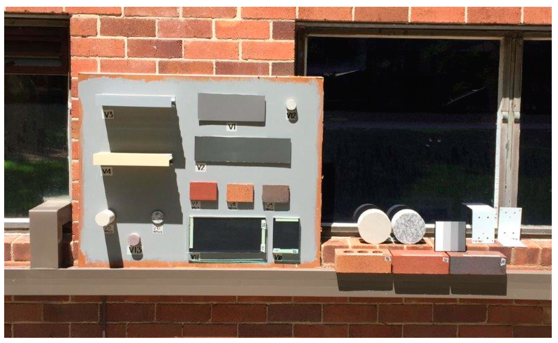
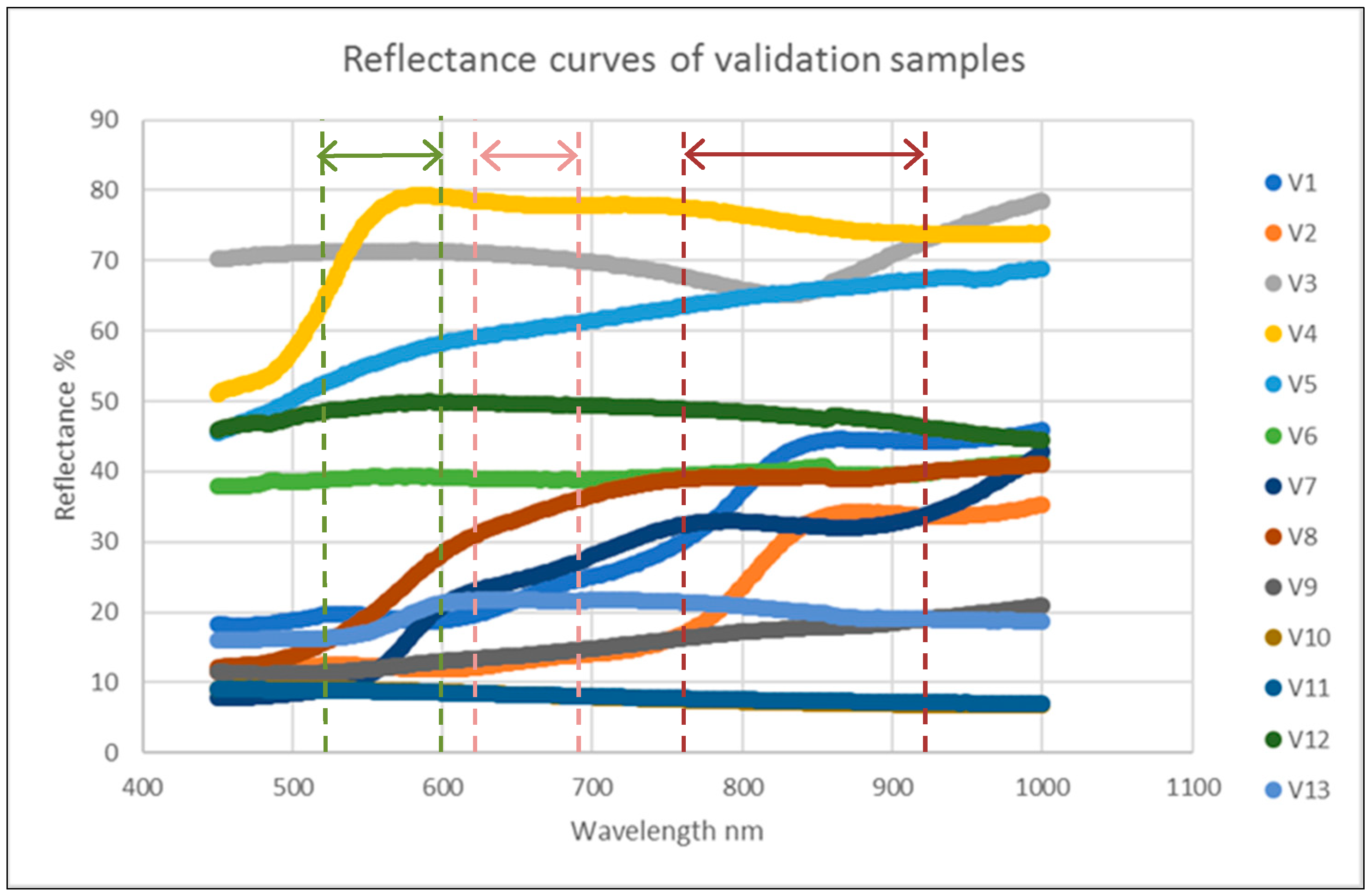
The measured (M) and predicted (P) mean spectral reflectance values of the 13 validation samples for all camera wavebands using the Dulux-derived EL2 are shown in

Table 15. Measured (M) and EL2-predicted (P) mean spectral reflectance (%) of 13 validation samples using EL1_Dulux intercept.

Waveband	Green			Red			NIR
Sample ID	M	P	AR1	M	P	AR	M	P	AR
V1	19.237	37.778	18.541	22.516	28.898	6.382	40.701	52.101	11.400
V2	12.196	27.145	14.949	13.198	17.670	4.472	28.877	39.703	10.826
V3	71.318	70.411	0.907	70.558	62.952	7.606	67.495	59.313	8.182
V4	75.261	69.702	5.560	77.969	91.490	13.521	75.396	90.843	15.447
V5	55.660	62.596	6.936	60.285	62.741	2.456	65.566	61.489	4.077
V6	39.165	44.223	5.058	38.892	42.304	3.412	39.834	41.017	1.184
V7	13.509	26.531	13.022	25.181	34.055	8.874	32.567	36.513	3.946
V8	21.444	32.155	10.710	33.965	40.947	6.981	39.210	41.689	2.479
V9	12.133	20.282	8.149	14.027	19.200	5.173	17.659	22.848	5.189
V10	8.861	19.832	10.971	8.223	13.064	4.841	7.149	29.292	22.143
V11	8.714	20.409	11.694	8.230	11.781	3.551	7.431	33.470	26.039
V12	49.377	64.151	14.775	49.592	62.009	12.416	47.882	52.978	5.097
V13	18.297	39.395	21.098	21.664	42.434	20.771	20.089	35.495	15.406
Mean	31.167	41.124	10.952	34.177	40.734	7.728	37.681	45.904	10.108
Sum AR			142.37			100.46			131.41
RMSE 1			12.228			9.177			12.561
d1			0.920			0.960			0.892

¹ AR: absolute residual. RMSE and d from [129].

below. Common statistical measures of correlation (Pearson’s r and Spearman’s rho), predictive precision (coefficient of determination, R²), distribution difference (Mann-Whitney’s U test) and prediction accuracy (Willmott’s index of agreement d, root mean square (RMSE) and mean absolute error (MAE)) are shown in

Table 16. Rank correlation and OLS regression statistics M-P from Table 15 data.

Statistic	Green		Red		NIR
Rank Correlation
Mann-Whitney U 1	Uc = 45	U = 54	Uc = 45	U = 69	Uc = 45	U = 64
Test result		U > Uc		U > Uc		U > Uc
Z-score	1.53846		0.76923		1.02564
p-value	0.12356		0.4413		0.30302
Spearman’s rho (rs)	0.945		0.940		0.967
OLS regression M-P
RMSEs 1	5.993		6.346		9.261
MAE	4.893		4.188		8.092
Pearson’s r	0.966		0.960		0.900
R2	0.933		0.922		0.810
d	0.982		0.979		0.945
Intercept (a)	−18.372		−4.81		−13.878
Slope (b)	1.2046		0.9224		1.1232

¹ RMSEs from [129]. U test: no statistical difference in distributions at 95% confidence level.

for evaluation of model performance [128,129,137] based on the OLS regression of measured against EL2-predicted reflectance values [138].

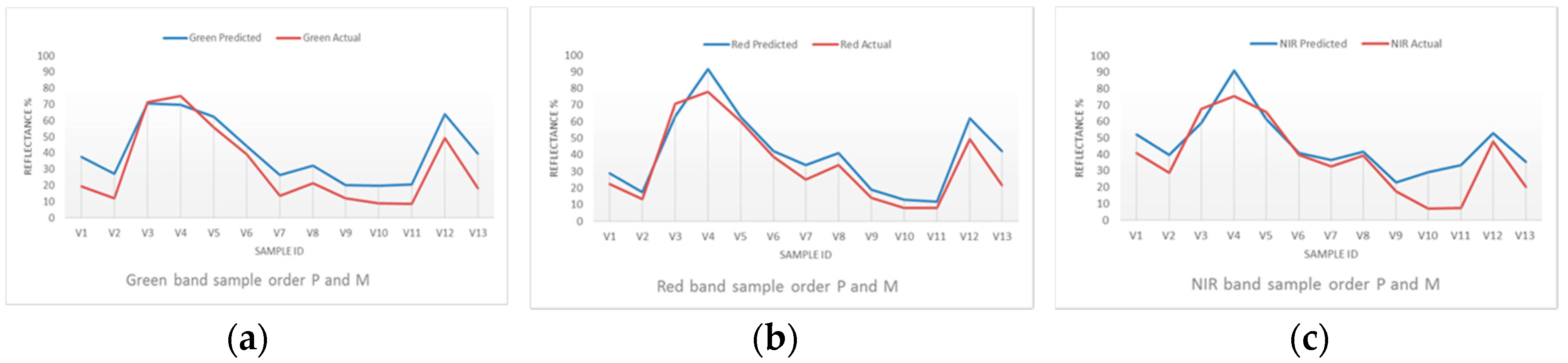
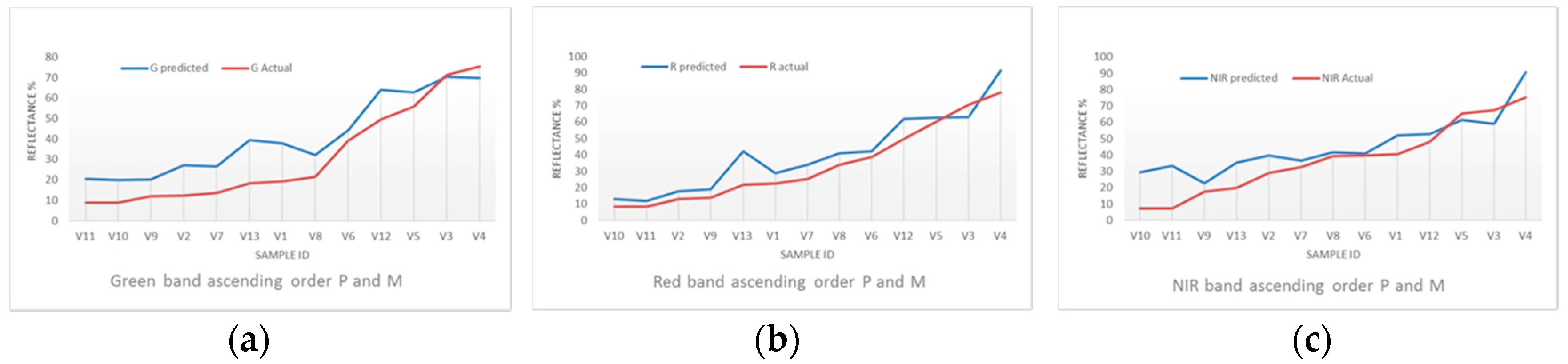
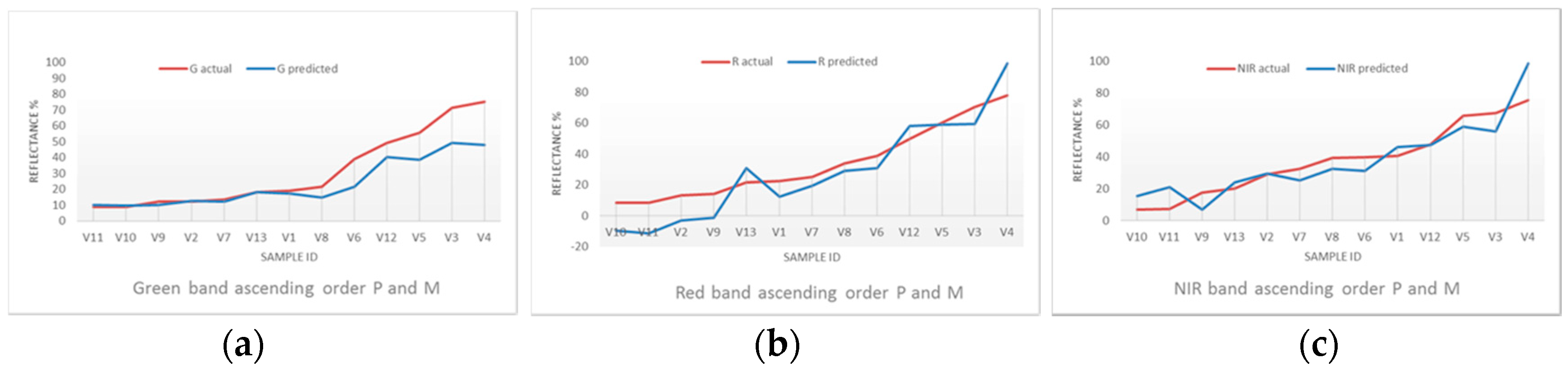
Plots of the measured and Dulux EL2 equation-predicted mean spectral reflectance values of the 13 validation samples are shown in Figure 9 and Figure 10 below.

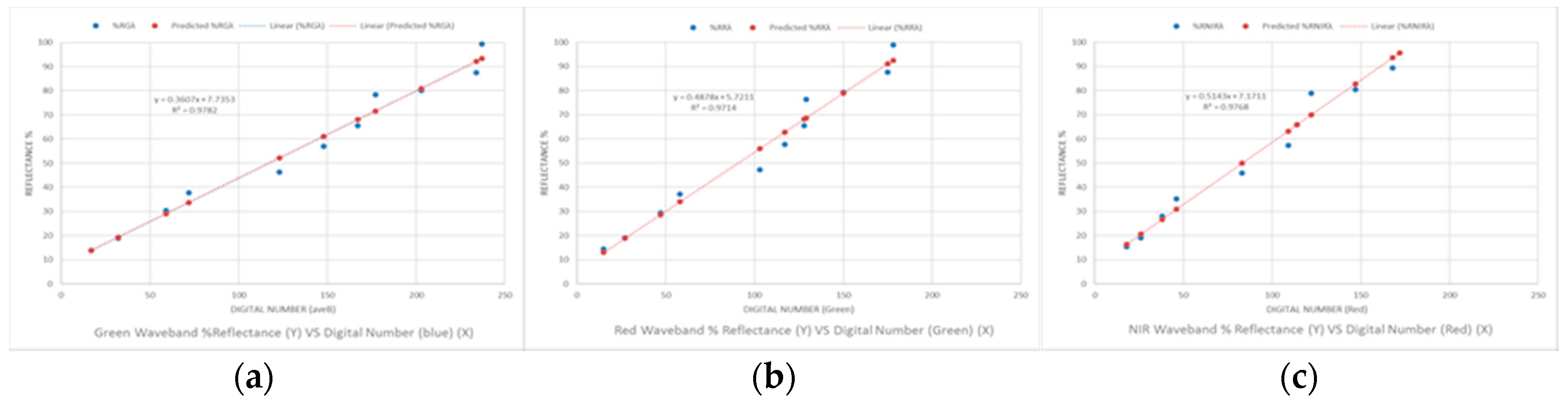
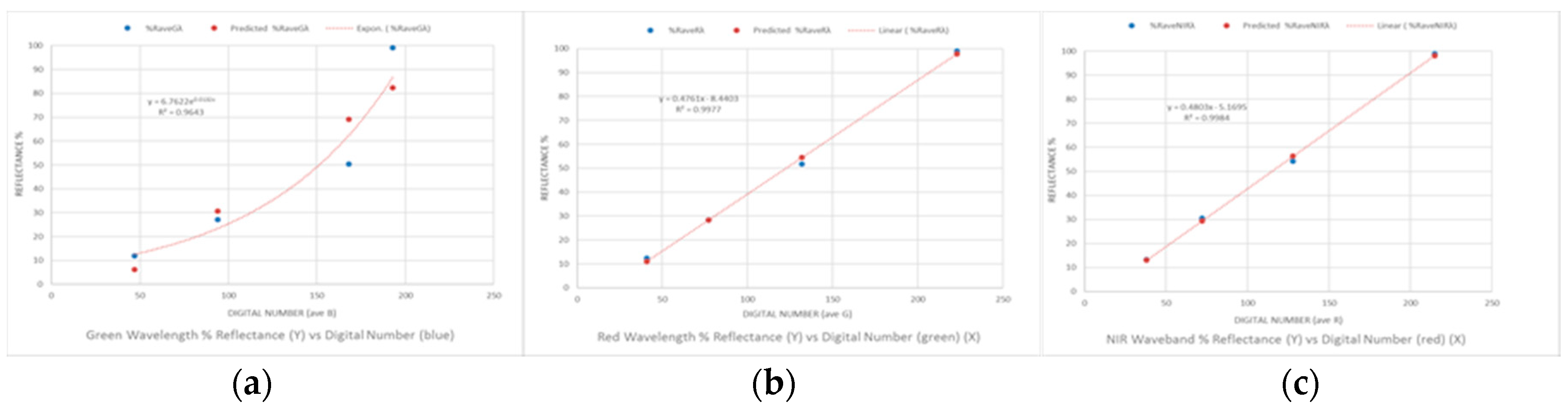
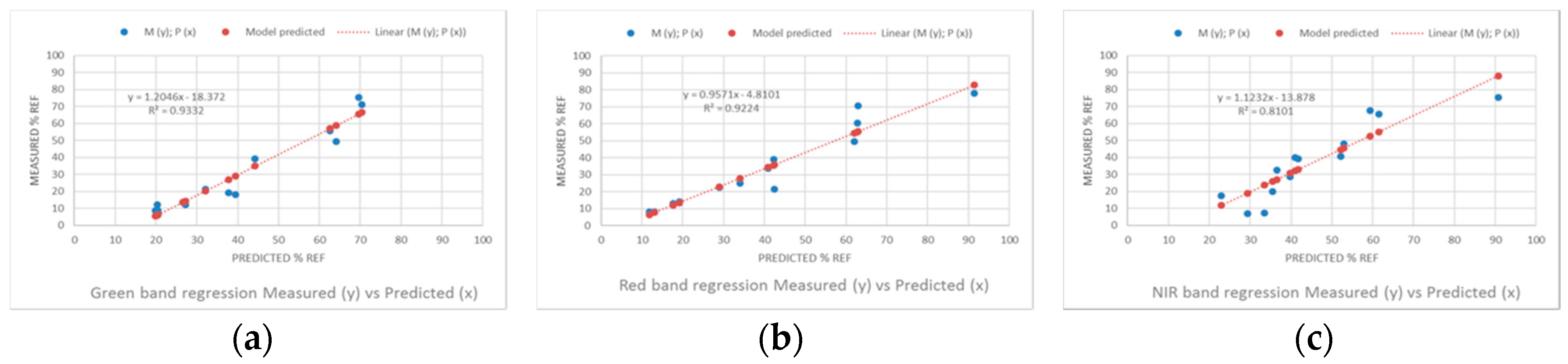
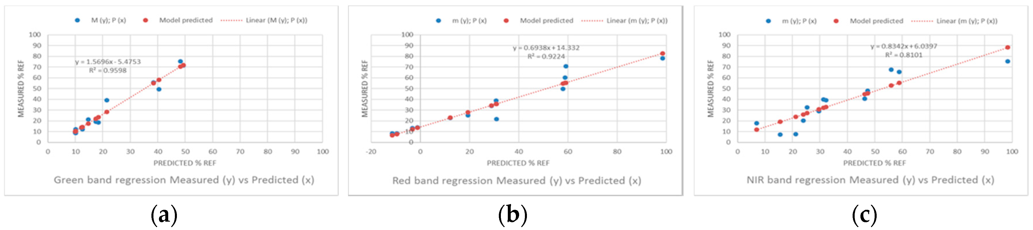
The OLS plots of measured (M) regressed against predicted (P) reflectance values per camera waveband are shown in Figure 11 below.

The measured and predicted mean spectral reflectance values of the 13 validation samples for the three camera wavebands using the intercept value from the Spectralon-derived EL2 equation and prediction model evaluation statistics are shown in

Table 17. Measured (M) and EL2-predicted (P) mean spectral reflectance (%) of 13 validation samples using EL1_Spectralon intercept.

Waveband	Green			Red			NIR
Sample ID	M	P	AR	M	P	AR	M	P	AR
V1	19.237	17.527	1.712	22.516	12.275	10.241	40.701	46.276	5.576
V2	12.196	12.512	0.315	13.198	−3.218	16.416	28.877	29.583	0.705
V3	71.318	49.314	22.003	70.558	59.251	11.307	67.495	55.987	11.507
V4	75.261	48.218	27.043	77.969	98.619	20.649	75.396	98.442	23.046
V5	55.660	38.494	17.166	60.285	58.960	1.325	65.566	58.917	6.649
V6	39.165	21.499	17.665	38.892	30.768	8.124	39.834	31.352	8.481
V7	13.509	12.270	1.239	25.181	19.389	5.792	32.567	25.287	7.280
V8	21.444	14.665	6.779	33.965	28.896	5.070	39.210	32.257	6.953
V9	12.133	10.065	2.068	14.027	−1.103	15.130	17.659	6.887	10.772
V10	8.861	9.922	1.062	8.223	−9.568	17.791	7.149	15.564	8.415
V11	8.714	10.106	1.391	8.230	−11.338	19.568	7.431	21.190	13.759
V12	49.377	40.439	8.938	49.592	57.950	8.358	47.882	47.458	0.424
V13	18.297	18.448	0.152	21.664	30.948	9.284	20.089	23.916	3.827
Mean	31.167	23.345	8.272	34.177	28.602	11.465	37.681	37.932	8.262
Sum AR			142.37			100.46			131.41
RMSE			12.228			9.177			12.561
d			0.920			0.960			0.892

and

Table 18. Rank correlation and OLS regression statistics M-P from Table 17 data.

Statistic	Green		Red		NIR
Rank correlation
Mann-Whitney U 1	Uc = 45	U = 73	Uc = 45	U = 70	Uc = 45	U = 80
Test result		U > Uc		U > Uc		U > Uc
Z-score	0.5641		0.71795		0.20513
p-value	0.57548		0.47152		0.83366
Spearman’s rho (rs)	0.945		0.940		0.967
OLS regression M-P
RMSEs	4.648		6.346		9.261
MAE	3.442		4.188		8.092
Pearson’s r	0.979		0.960		0.900
R2	0.960		0.922		0.810
d	0.989		0.979		0.945
Intercept (a)	−5.475		14.332		6.039
Slope (b)	1.5696		0.6938		0.8342

¹U test: no statistical difference in distributions at 95% confidence level.

below.

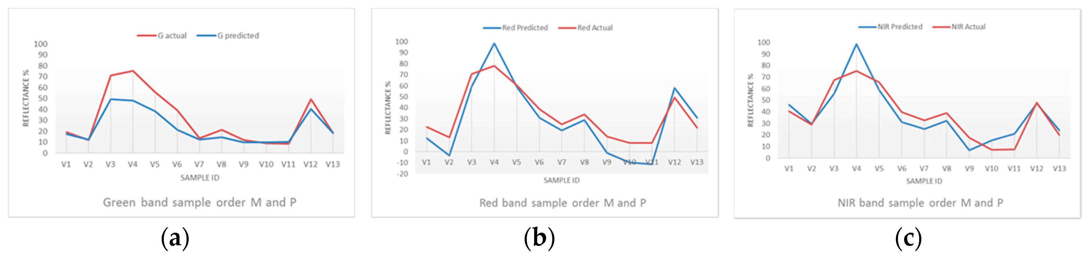
Plots of the measured and Spectralon EL2 equation-predicted mean spectral reflectance values of the 13 validation samples are shown in Figure 12 and Figure 13 below.

The OLS plots of measured (M) regressed against predicted (P) reflectance values per camera waveband are shown in Figure 14 below.

In addition to linear covariance tests (r, R², intercept a and slope b), OLS model prediction error was evaluated using supplementary measures recommended by [128,129]. These include the systematic root mean square error (RMSEs) and the unsystematic root mean square error (RMSEu). For “good” model performance the RMSE should be low, RMSEs should tend to zero, RMSEu should approach RMSE and Willmott’s index of agreement (d), a measure of prediction accuracy, should approach unity [128]. MAE provides an estimate of mean differences between measured and predicted values and is an “intuitive”, reliable measure of average model prediction error [139]. While RMSE is a widely reported measure of average model error, it is less reliable than MAE since it exaggerates differences due to higher sensitivity of RMSE to outliers [129,140] and due to the inconsistent variance of RMSE with average error [139].

Table 19. Summary statistics of EL2-equations and OLS model performance.

Equations	EL2-Equation Measures				OLS Regression Parameters				OLS Difference Measures
	1 Mm	1 Pm	RMSE	MAE	r	R2	a	b	RMSEs	RMSEu	MAE	d
GreenDulux	31.167	41.124	12.228	10.952	0.966	0.933	−18.372	1.205	5.993	10.659	4.893	0.982
GreenSpectralon	31.167	23.345	12.279	8.272	0.979	0.960	−5.475	1.570	4.649	11.364	3.442	0.989
RedDulux	34.177	40.734	9.177	7.728	0.960	0.922	−4.81	0.922	6.346	6.630	4.188	0.979
RedSpectralon	34.177	28.602	12.830	11.465	0.960	0.922	14.332	0.6938	6.346	11.151	4.188	0.979
NIRDulux	37.681	45.904	12.561	10.108	0.900	0.810	−13.878	1.123	9.261	8.486	8.092	0.945
NIRSpectralon	37.681	37.932	10.014	8.262	0.900	0.810	6.038	0.834	9.261	3.810	8.092	0.945

¹ M_m = Measured mean, P_m = Predicted mean.

below summarizes the performance of both models per waveband to evaluate the most accurate and precise predictive EL equations.

Comparing the model results for the Green waveband, the lower Spectralon-derived OLS equation RMSEs and MAE, higher RMSEu with higher d in agreement with higher regression R² indicate its unambiguous predictive superiority (bold in Table 19). Comparing the model results for the Red waveband, considering equivalence of linear regression measures RMSEs, MAE and d, the lower Dulux-derived EL2-equation MAE (lowest of all wavebands) and regression parameters (intercept a (−4.81) and slope b (0.922)) closer to the ideal 1:1 correspondence line (when a = 0 and, more importantly, b = 1) for goodness of fit [141] indicate its superior predictive precision and accuracy (bold in Table 19). The above interpretation was supported when comparing the additive and proportional components [128] of the MSEs for each model.

Comparing the results for the NIR waveband, despite a lower MAE for the EL2-Spectralon equation estimates and considering the equivalence of OLS correlation and difference measures, the significantly lower RMSEu for Spectralon-derived OLS suggests that the Dulux-derived EL2 equation contains proportionally less systematic error overall and hence improved accuracy (bold in Table 19). This conclusion is augmented by computation of the ratio MSEs/MSE [129] that indicates that the Dulux-derived NIR predictive model contains a significantly lower proportion (54.4% vs. 85.5%) of systematic error and hence greater comparative model accuracy.

In summary, the optimal predictive models per waveband indicate a strong monotonic agreement (0.940 < Spearman’s Rho > 0.967) and linear association (0.900 < Pearson’s r > 0.966) between the measured and EL2-predicted reflectance values that confirm a near-perfect positive agreement between pairs of samples of ranked scores and a strong linear correlation [142]. The regression measures imply distribution near-equivalence and high confidence in trend predictions [143]. Regardless of the residual magnitudes, the distributions (Figure 9, Figure 10, Figure 12 and Figure 13) show a strong positive agreement that supports reflectance predictions on a relative (high/low) scale. The non-parametric Mann-Whitney U-test for difference between two independent groups exhibits no statistically significant difference in distributions at the 95% confidence level, reinforcing the above interpretation [144]. The coefficients of determination (R²) of the OLS models for all wavebands exceed 81% (NIR). Green and Red band R² exceed 92.2%. This suggests stronger agreement in the visible bands between measured and predicted values and higher confidence in the precision of the linear covariance between measured and predicted values [138].

Comparative Assessment of Measured and EL2 Predicted Reflectance Distributions

The mean bias error (MBE) [139] between measured and Dulux-derived EL2 equation predicted reflectance values for all wavebands indicates a systematic overestimation of measured values (Figure 9 and Figure 10), a trend corroborated by the regression model (Figure 11) and regression slope and intercept parameters (Table 16). The overestimation bias derives from the camera calibration model (Table 6). However, higher reflectance samples (V3 (nominal reflectance 70%); V4 (75%) and V5 (60%) in Table 15) underestimate measured values. Underestimation of high-albedo surfaces by the EL method has been reported previously [94]. Sample V13, red Granite stone (nom. reflectance 20%) exhibits the largest absolute residual for the Green and Red wavebands. The high error may be theoretically accounted for by the reflectance anisotropy common to natural materials [135] in combination with artifacts of the prediction model. However, the low absolute residual magnitude of the Spectralon-derived estimate for the same sample (Table 17) implicates the latter. The largest absolute residual for the NIR waveband (Dulux-derived) occurs for sample V11, 5 mm Clear Glass (nom. reflectance 8%). The specular behaviour of glass at oblique incident angles (as occurred in the validation experiment, where the solar altitude exceeded 65°) may account for the larger difference in the NIR region [48]. Further, the low measured reflectance of glass falls outside the reflectance data range used to build the EL equations which may increase prediction error for this sample [98].

The MBE between measured and Spectralon-derived EL2 equation predicted reflectance values for the Green and Red wavebands indicates a systematic underestimation of measured values (Figure 12 and Figure 13), a trend corroborated by the regression model (Figure 14) and regression slope and intercept parameters (Table 18). The underestimation bias derives from the camera calibration model (Table 7). MBE for the NIR waveband indicates marginal average overestimation of measured reflectance values, with some exceptions. Sample V13, red granite stone, is overestimated in all three wavebands and largest for the Red waveband. The highest reflectance sample, Sample V4 (powder coated aluminium, cream colour, nominal reflectance 75%), exhibits the largest absolute residual for all camera wavebands and is overestimated in the Red and NIR bands. The Spectralon model prediction of maximum error per sample is inconsistent with the Dulux-derived response to maximum error but consistent with prior studies that found predictions of high albedo surfaces have higher errors than low albedo surfaces [48].

The range of measured mean spectral reflectance values (approx. 7% to 78%) of the validation samples across all wavebands was comfortably within the upper reflectance limit of the calibration targets used in the development of the predictive equations (approx. 99% for EL1 and 89% for EL2). However, the two glass samples had measured reflectance values below the lower limit of the model data range (approx. 12% for EL1). For all samples (excluding glass) the predicted values were interpreted within the limits of the calibration equations [88,98].

4. Discussion

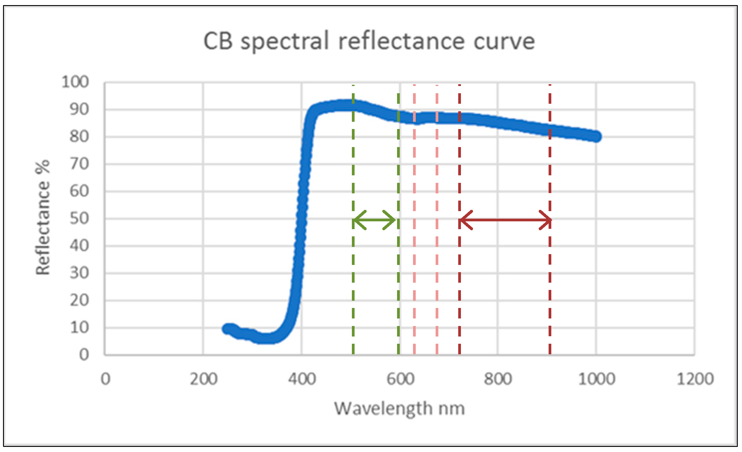
In this study a terrestrial application of the EL method [88] was developed to radiometrically calibrate and validate close-range remotely sensed images of vertical surface materials obtained from a narrow FOV MS camera using a single in-situ calibration target [98]. The y-intercept of the camera response function, although variable with camera calibration target properties, was shown to be the minimum reflectance detectable by the camera sensor per waveband and was used as the lower data point. The second coordinate of the EL equation was derived from the per-waveband spectral reflectance values and DNs of the CB. While the CB was assumed to be Lambertian, the spectrophotometer measurements of the CB indicated that mean spectral reflectance was unequal across sensor wavebands (Table 9) with a declining reflectance trend observed from shorter (visible) to longer (NIR) wavelengths (Figure 6) necessitating a separate EL equation for each waveband [98]. The optimal EL2 equations per waveband (Table 19) strongly linearly correlated (0.900 < r > 0.979) per-pixel spectral reflectance to image DNs with absolute prediction accuracies (7.728% < MAE > 10.108%) within the range reported in the literature [88,94].

Theoretically, improvements in accuracy are achievable if the calibration target is accurately characterized [136] and more than one in-situ calibration target is used [132] and future experimental design could, without much logistical effort, incorporate additional portable near-Lambertian targets, selected for spectral uniformity within sensor wavebands [135]. Instrument characteristics have been identified as a common source of experimental uncertainty [145]. Accuracy improvements may result from the optimisation of camera settings (i.e., manual exposure) within the limitations of the sensor radiometric resolution [92,98,134] and from corrections for sensor background noise and vignetting [87]. However, the anticipated absolute accuracy improvements are not crucial for the “relative magnitude” of elements of the scene approach adopted here where distribution equivalence is more highly prized.

The variable per-waveband mean spectral reflectance of the CB, characterized by greater reflectance in the visible band (Table 9), its smooth, low-sheen surface finish (potentially with a non-negligible specular component at large incident angles [48,146]) and the non-uniform Tetracam ADC CMOS sensor response function to different sensor bandwidths (with lowest sensitivity in the Green waveband) may account for the relative distribution of errors per waveband [86,87]. Importantly, due to near-horizontal viewing geometry, it is speculated that the accuracy of the reflectance recovery computations is strongly influenced by angular and adjacency effects (in particular from ground reflections) [75,85] and the impacts of in-situ spectral, diffuse and direct effects that are not explicitly accounted for in the laboratory measurements [62,146,147].

The majority of prior ground- or UAV-based studies utilising the vicarious EL method with narrow FOV MS sensors for reflectance recovery have been concerned with horizontal vegetated surfaces [86,87,95,96,102] and fewer with horizontal urban surfaces [48,104]. Furthermore, the use of the EL method applied to terrestrial close-range MS sensors with near-horizontal viewing geometry of urban building facades has not been previously reported. However, there is growing interest in the use of ground-based, close range narrow FOV sensors for retrieval of the spatio-temporal optical and thermal characteristics of vertical surfaces at the facet and sub-facet scales for building damage assessment [148], geological surveys [85] and urban climatology [78].

As there is a gap in the literature addressing, and no standard method exists for, facet and sub-facet scale terrestrial reflectance recovery from real building facades, the value of this paper is its contribution to the development of a logistically simple, replicable, validated reflectance recovery method, with explicit error magnitude and source estimation, suitable for climatology studies of building facades using a single mobile calibration target and high-resolution close-range images obtained from a relatively low-cost MS camera. However, since each camera has a unique sensor response-function [92] and irradiance may vary under different environmental conditions, the determination of the relationship between reflectance and DNs necessitates the computation of new equations for each new sensor and every unique environment [98].

5. Conclusions

This paper described a novel application of the EL method for radiometric calibration of a relatively low-cost MS sensor applied to close-range images of vertical urban surface materials. The performance of the single-target EL calibration equations was evaluated and quantified using validation samples of common building materials. Confidence in the precision and accuracy of the EL equations per-waveband was assessed using covariance statistics and error measures [128,129,137] and absolute prediction accuracies (7.728% < MAE > 10.108%) were within the range reported in the literature [88,94,149] and above prediction accuracies (15–20%) reported for single-target calibration methods [88,103].

Based on the optimum equations (Table 19) the results are encouraging and indicate that the prediction equations (Table 11 and Table 12) satisfactorily characterize the per waveband reflectance differences of commonly used materials found on Australian building facades. For example, dry-pressed clay bricks (samples V7, V8, and V9, Table 14) are frequently used in low to medium-rise construction of residential buildings in Sydney and are satisfactorily predicted in the green waveband within a range of 1.24% to 6.68% absolute error (AE) (Table 17) and OLS model absolute residuals (OMAR) of 0.27%, 3.9% and 1.8% respectively. Importantly, the NIR waveband reflectance values are satisfactorily predicted within a range of 2.48% to 5.19% AE (Table 15) and OMAR in the range of 5.4% to 6.2%. This relative predictive strength is significant since dry-pressed clay bricks are both pervasive and more reflective in the NIR region (Table 14 and Figure 8).

Dark-grey pre-painted steel sheeting (sample V2) is another prevalent material used for building facade cladding that is more reflective in the NIR region (Table 14 and Figure 8). Green and NIR waveband reflectance values are satisfactorily predicted with a 0.32% and 0.71% AE (Table 17) and OMAR of 1.96% and 1.84% respectively. Glass (samples V10 and V11) is reasonably well predicted in the visible spectrum with a 1.06% and 4.84% AR in the Green (Table 17) and Red (Table 15) bands with an OMAR of 1.24% and 0.53% respectively for sample V10.

While the results confirm the findings of prior studies supporting the utility of a single in-situ target for radiometric calibration [86,98] it may be concluded from method and model evaluation that improvements in measurement protocols and calibration target specification would reduce prediction model error, although the anticipated absolute accuracy improvements are not warranted here since the “relative magnitude” of elements of the scene and distribution equivalence are desired for the development of a larger statistical model. The regression statistics (Table 16, Table 18 and Table 19) imply distribution near-equivalence between measured and predicted reflectance values and high confidence in trend predictions. This demonstrates that a single-target EL method can be applied to recover spectral reflectance from terrestrial close-range MS images of vertical surfaces with satisfactory results.