Land Use Change and Its Impacts on Land Surface Temperature in Galle City, Sri Lanka


Department of Environmental Management, Faculty of Social Sciences and Humanities, Rajarata University of Sri Lanka, Mihintale 50300, Sri Lanka
Climate 2020, 8(5), 65; https://0-doi-org.brum.beds.ac.uk/10.3390/cli8050065
Submission received: 10 April 2020
/
Revised: 14 May 2020
/
Accepted: 14 May 2020
/
Published: 18 May 2020
(This article belongs to the Special Issue Landscape and Climate Change)
Abstract
:This study investigated the spatiotemporal changes of land use land cover (LULC) and its impact on land surface temperature (LST) in the Galle Municipal Council area (GMCA), Sri Lanka. The same was achieved by employing the multi-temporal satellite data and geo-spatial techniques between 1996 and 2019. The post-classification change detection technique was employed to determine the temporal changes of LULC, and its results were utilized to assess the LST variation over the LULC changes. The results revealed that the area had undergone a drastic LULC transformation. It experienced 38% increase in the built-up area, while vegetation and non-built-up area declined by 26% and 12%, respectively. Rapid urban growth has had a significant effect on the LST, and the built-up area had the highest mean LST of 22.7 °C, 23.2 °C, and 26.3 °C for 1996, 2009, and 2019, correspondingly. The mean LST of the GMCA was 19.2 °C in 1996, 20.1 °C in 2009, and 22.4 °C in 2019. The land area with a temperature above 24 °C increased by 9% and 12% in 2009 and 2019, respectively. The highest LST variation (5.5 °C) was observed from newly added built-up area, which was also transferred from vegetation land. Meanwhile, the lowest mean LST difference was observed from newly added vegetation land. The results show that the mean annual LST increased by 3.2 °C in the last 22 years in GMCA. This study identified significant challenges for urban planners and respective administrative bodies to mitigate and control the negative effect of LST for the long livability of Galle City.
1. Introduction
Unlike rural areas, urban centers are much more complex and dynamic as they provide the highest rate of socio-economic footprints [1]. As cities are the central locations for capital, administration, infrastructure, education, information, and transportation, researchers have paid comprehensive attention to urban studies from a wide variety of disciplines over the past few decades [2]. According to the scientific literature in the Web of Science database, a detailed search of cities began early in the 1920s [2]. From then, many attempts have been made by researchers regarding urban studies from various viewpoints. Among them, research related to the spatiotemporal changes of land use land cover (LULC) and its impact on land surface temperature (LST) were highlighted, and details of this can be found elsewhere [3,4,5].
Multiple previous studies have well proven that urbanization is the driving force for changing LULC in a city [6,7,8,9]. Owing to the resource pool and livability attraction, the number of city populations has dramatically increased in the last few decades [10]. The United Nations has forecasted that 66% of the global population is expected to be lodged in cities in 2050 [10]. On the basis of this context, cities attempted to provide services (job, settlement, transportation, and so on) by acquiring land resources from the city and its periphery area. This was caused by several externalities, which predominantly addressed it as “LULC change issues” [4,6]. Many socio-economic and environmental issues are led by the unplanned LULC changes in an urban area. Some of these issues are irreversible and have reached alarming levels [5]. Increasing land surface temperature (LST) is one of the urban issues. Moreover, this issue is accelerated by unplanned LULC changes, especially in developing countries. Anthropogenic heat sources are prominent on the urban surface, which is covered by impenetrable materials, including roads, parking lots, industrial and commercial areas, and so on. Impenetrable materials encourage both radiation rapping during the day [11] and re-radiating, which is known as “heat back”, at night [12]. This phenomenon is majorly the reason LST increases in urban areas, as proven by research [13]. Consequently, city planners and researchers are concerned about elevated temperature owing to its effect on socio-economic (human health and energy [14,15]) and environmental (air quality and water [4,16]) attributes required for the wellbeing of urban dwellers [17]. Thus, research on LST and its effect is becoming the major focus among the information-avid scientific community.
Identification of the LST pattern by temporal viewpoint is essential to understand LST behavior and its responsiveness for LULC changes [18,19,20,21]. Several researchers have also stated that multiple time points Landsat data set provides a more accurate temporal comparison on LST rather than a single snapshot of Landsat image [18,22]. However, the acquisition of multiple time points data is not an easy task owing to cloud disturbances, especially in the tropical region. This obstacle was managed using a more sophisticated and user-friendly mapping system, which is known as the Google Earth Engine (GEE) [22]. It has various kinds of remote sensing (RS) applications, including over 30 years of Landsat historical data archives [23,24,25]. There are several benefits of RS, including (i) being freely available [26], (ii) solution for data unavailability, (iii) being applicable to inaccessible areas, (iv) less fieldwork, and (v) software compatibility. Thus, GEE-based Landsat data were utilized for the calculation of annual median LST and LULC information. Excluding this, traditional research based on field activity is time-consuming, not applicable for large scale research, and not cost-effective [27].
Changing of LULC is a continuous process on Earth’s terrestrial surface [28,29]. Nevertheless, its changes in an urban environment are quite different. Owing to the complex anthropogenic activities, a profound dynamic change in an urban area can be monitored. Generally, the urban area has expanded by acquiring lands from its surroundings. Moreover, LST responsiveness can indicate the difference even in the same urban area [19]. Hence, studying this dynamic system is much more important not only for understanding LST variation on LULC types, but also socio-economic and environmental implications. Additionally, different types of LCLU have their own LST behaviors [30,31]. Therefore, it is required to identify the composition of existing LULC as much as a precise level to compute its contribution to LST variations. Nevertheless, identification of land use and land cover types in a complex urban environment is a challenging task. Hence, theoretically roughness, practical oriented remote sensing (RS), and geographic information system-based LULC classification technique were widely used by researchers [19].
In this research, the Galle Municipal Council area (GMCA) was selected as the study area. Galle City is the landmark of the GMCA and is as popular as a coastal city. Mainly, it is accessible on both marine (natural harbor) and terrestrial surface (southern highway and west-coast line, which is known as Galle road or A2 road) [32]. As evidence suggests, GMCA has undergone rapid urban development over the last two decades [32]. In terms of population size and number of commuters, Galle is the fourth largest municipality [32] and the essential administrative capital of the Southern Province of Sri Lanka. It performs a number of functions including the regional administrative, education, and tourism industry, plus transportation and economic activities. Owing to these functionalities, a massive urban expansion and LULC changes have taken place in GMCA in the last two decades. However, research related to the land-use changes and its impact on LST was lacking in the study area. Regarding this content, the importance of GMCA was identified using literature [33,34,35], development plans [32], and field investigation. These were some factors that inspired the choice of this research title. In this empirical study, RS and GIS techniques are employed to detect spatiotemporal changes and land-use patterns. This is to answer the query of how the LULC has changed and its influence on LST variation in GMCA in 1996, 2009, and 2019. The purpose of this study was to compute how different urban LULC and their changes affect LST variation. The study also aims to find how these relationships compare and contrast between the spatial and temporal aspect.
2. Materials and Methods
This section is completed with a comprehensive explanation of the methodology and the materials used in the study. It goes from the study area to spatial calculation as seven sections by elaborating necessary steps.
2.1. Study Area
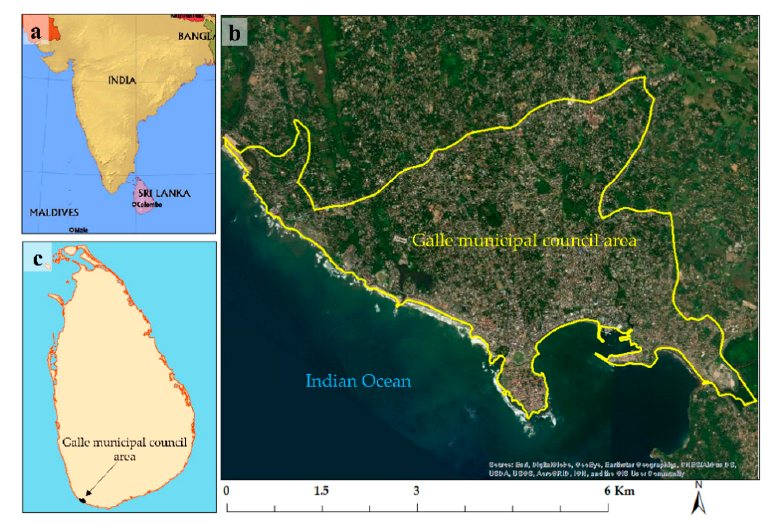
The seaside city of Galle is bordered by the Indian Ocean from south and southwest, and is the provincial capital city of the Southern province, Sri Lanka. It is located in the down south coast 116 km away from Colombo [32]. From the biophysical aspect, agroclimatic regain of the city goes within the wet zone. Moreover, the city experiences a monsoon distribution of rainfall, which receives 2377.9 mm per year [32]. The average daytime ambient temperature is 26.7 °C [32], while humidity ranges from 80% to 88% [32]. Excluding a few isolated hills, which are around 60–160 feet, other areas are lowland, including marshes and water bodies.
From the socio-economic viewpoint, Galle City is an active place where many inheritances live and work because of the main economic center located in the Southern province [33]. Galle natural harbor serves as one of the most dynamic regional ports and its only Sri Lankan port that facilitates yachts for pleasure. For its natural beauty and archaeological value, Galle City is a famous tourist destination for both locals and foreigners. In 1988, the United Nations Educational Scientific and Cultural Organization (UNESCO) declared the Galle fort as a world heritage site by naming it as the “Old Town of Galle and its Fortifications”. In this research, GMCA was selected (Figure 1) and is bounded by 6.025330° to 6.062277° latitude and 80.174328° to 80.250181° longitude, covering 1821 ha. Under the provisions of the urban council ordinance of 1865, Galle has been established as the third municipal council of Sri Lanka [32].
2.2. RS Data Acquisition
There might be a minor seasonal change in GMCA that can slightly affect the land cover, especially for vegetation and water bodies. However, on the basis of the information given in Table A2, significant air temperature variations were not observed. In addition, there were no extreme cases (snow or drought). Further, past researchers have also hypothesized that the use of more Landsat images to cover the year would produce reliable data sets [18,25]. Moreover, such kinds of datasets can be used for temporal comparison, with more details provided in the introduction section. In this regard, a cloud-based remote sensing data platform GEE was used to generate annual average data sets [36,37]. GEE is an application programming interface, and it is a free tool. It provides radiometric-calibrated and atmospheric-corrected Landsat level 2 data powered by United States Geological Survey (USGS) [38]. Additionally, GEE supports various kinds of spatial analysis and applications, including time-series analysis [36]. In the data acquisition process, the following steps were accomplished.
- i.
- Annual average Landsat data sets were selected by applying the study area as a geometry region. The masking method was applied to remove the cloud areas owing to cloud disturbance in the available Landsat imageries.
- ii.
- iii.
- iv.
- Classification of LULC and derivation of LST was carried out using the above basic data sets.
2.3. Image Classification and LULC Change Detection
Updated LULC information was not available to cover the investigation period. This obstacle was managed using image classification techniques, as numerous studies have demonstrated [39,40]. The process is complex and requires the consideration of several steps. First, it involves selecting the appropriate classification method. Though there are various kinds of classification techniques; the random forest (RF) method is still popular among researchers who attempt to identify the LULC information from medium resolution remotely sensed data [41,42]. RF is a machine learning method that supports the pixel-oriented supervised classification environment. Owing to popularity, theoretical roughness, and applicability with selected data sets, the RF method was chosen. Second, four types of LULC (built-up, vegetation, water, and others) were classified, and the attributes of each type are presented in Table 1.
2.4. Accuracy Assessment of Classification
Four hundred training sampling points were generated by a stratified random sampling method for each year [19], and an accuracy assessment was conducted for each LULC type. Google Earth’s historical imageries were facilitated for creating ground reference data in 2019 and 2009. Owing to the low spatial resolution on Google Earth’s historical imageries for 1996, the information was not clear. Thus, LULC information was observed with visual interpretation by generating different band combinations [19,47]. Finally, overall accuracy was calculated for each year using a confusion matrix.
2.5. LULC Changes
LULC change detection is a significant factor in the urban study, environmental change, and urban expansion monitoring. Timely and precise LULC change determination is a quite challenging task, but it is essential for a better understanding of the temporal changes [19,40]. In this research, the post-classification change detection method was chosen, and cross-tabulation was done by selecting pixel by pixel in pairs of two different years (1996 vs. 2009, and 2009 vs. 2019). This method was commonly used in similar studies, and its details can be found elsewhere [3,19].
2.6. Computation of LST
LST was calculated using pre-processed Landsat datasets (Section 2.2). Annual median at-satellite brightness temperature in Kelvin was transformed into degrees Celsius (°C) as emissivity corrected LST. In the process, the following steps were completed.
First, the normalized difference vegetation index (NDVI) [48] was calculated (Equation (1) [49]) in order to compute the proportion of vegetation.
where refers to the surface reflectance values of band 4 (Landsat-5 Thematic Mapper and band 5 (Landsat-8); and refers to the surface reflectance values of band 3 (Landsat-5 Thematic Mapper) and band 4 (Landsat-8 Operational Land Imager).
Second, the proportion of vegetation was calculated [47,50,51] (Equation (2)).
where represents the amount of vegetation or proportion of vegetation, NDVI represents normalized difference vegetation index, represents the minimum values of the NDVI, and represents the maximum value of the NDVI.
Third, land surface emissivity (ε) was calculated from Equation (3).
where is land surface emissivity and m and n are the functions of soil emissivity and vegetation emissivity, respectively. is proportion of vegetation (Equation (2) [50]). ; and , where and are the soil emissivity and vegetation emissivity, respectively. In this study, we used the result of Sobrino et al. (2004) [51] for m = 0.004 and n = 0.986.
Fourth, and finally, emissivity corrected LST was calculated (Equation (4)).
where is at-satellite brightness temperature in Kelvin; λ is the central-band wavelength of emitted radiance (11.45 μm for band 6 [52,53] and 10.895 μm for band 10 [54]); is h × c/σ (1.438 × 10⁻² m K), where σ is the Boltzmann constant (1.38 × 10⁻²³ J/K), h is Planck’s constant (6.626 × 10⁻³⁴ Js), and c is the velocity of of light (2.998 × 10⁸ m/s); and ε is land-surface emissivity estimated using Equation (3) [51]. Then, calculated LST values (Kelvin) were converted to degrees Celsius (°C).
2.7. Spatial Calculations
Spatiotemporal changes of LST by LULC types were calculated to determine the responsiveness temperature according to landscape changes. In this approach, changes in BU and VG were mainly focused on the pairs of two different years. In the process, the following steps were carried out. First, five types of changes were identified as follows: persistence built-up (PBU), persistence vegetation (PVG), the gain of built-up from others (GBUO), the gain of built-up from vegetation (GBUVG), and the gain of vegetation from others (GVGO). Second, the mean LST of the above five types was extracted and compared with previous time points to determine the temporal variation of LST. Finally, graphs and tables were produced to present spatiotemporal changes of LST by LULC types in the GMCA. In this spatial calculation process, the water body was excluded owing to two reasons: (i) it covers only 1% of the study area and (ii) no significant changes were observed from changes detection analysis.
3. Results
The results are presented as tables (descriptive statistical), figures (map and charts) with comprehensive details, and the necessary explanation by text.
3.1. Dynamic of LULC
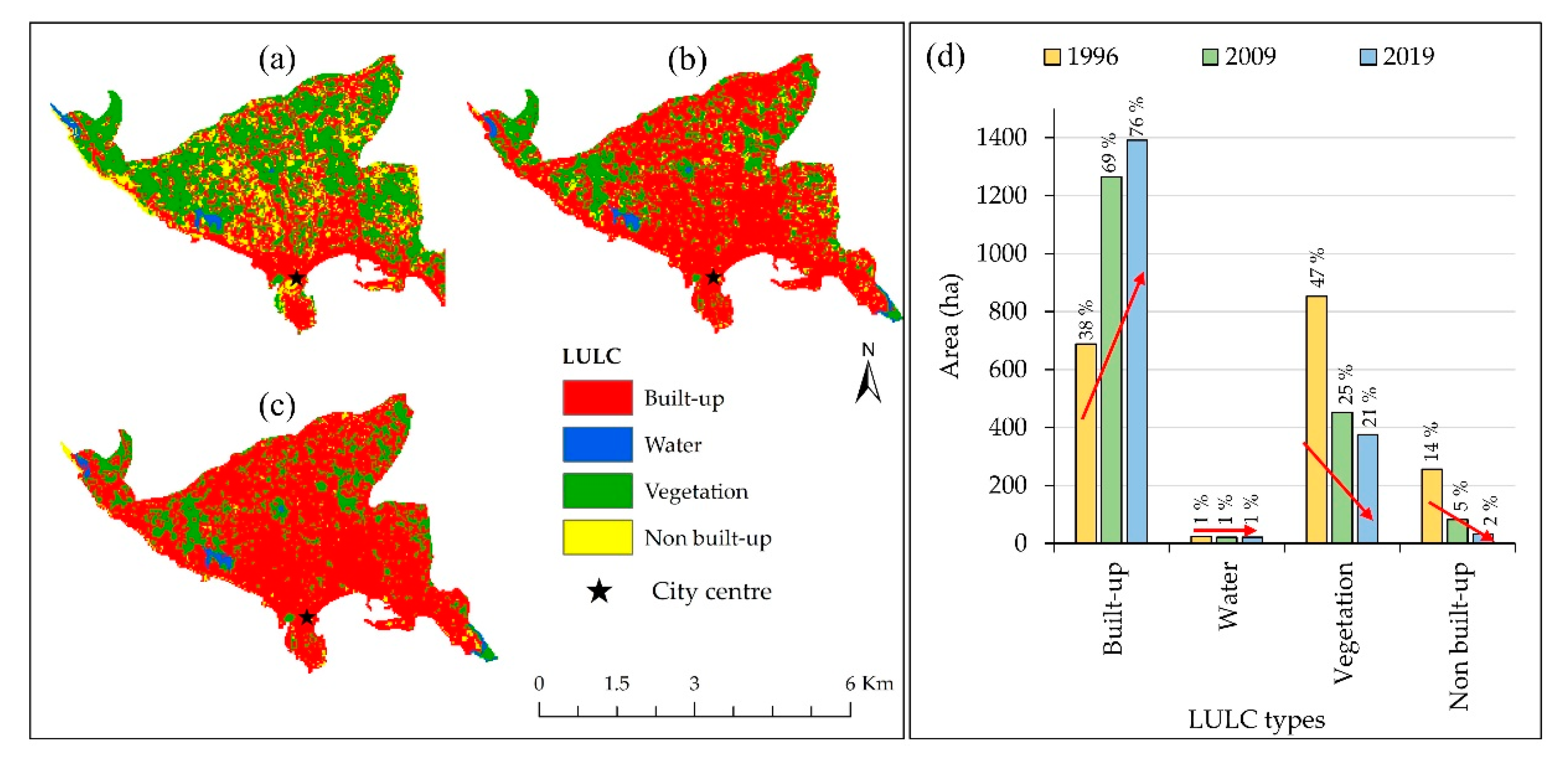
The overall accuracy of the LULC maps (Figure 2a–c) for 1996, 2009, and 2019 was 93.25%, 91.5%, and 96%, correspondingly. Spatiotemporal changes in LULC maps generated for the GMCA are presented in Figure 2a–c. Meanwhile, a descriptive statistic of the changes in land LULC and its percentage values are presented in Figure 2d. Mainly, BU areas steadily increased over the study period, starting from 628.4 ha (1996) to 1391.6 ha (2019). Rapid development was observed between 1996 and 2009, as shown in Figure 2d. About 577.5 ha (32%) of new BU land has been added from 1996 to 2009. Mainly, urban expansion has taken place in north, east, and northwest directions from the city center (Figure 2a–c). VG areas have gradually declined, and its temporal changes were observed as 852.1 ha (47%) in 1996, 452.3 (25%) in 2009, and 375.4 (21%) in 2019. The irregular spatial distribution pattern was observed from VG, but fairly higher density areas can be seen away from the main city, especially on the north side, as shown in Figure 2a–c. In 1996, NBU was 14% (255.8 ha) of the total area. However, it declined to 2% (32.7 ha) in the last two decades. The WB was only about 1%, and there were no significant changes in WB over the investigation period. Generally, a mixture of LULC types can be seen in both 2009 and 2009, rather than the isolated land fraction.
3.2. The Spatiotemporal Distribution Pattern of LST
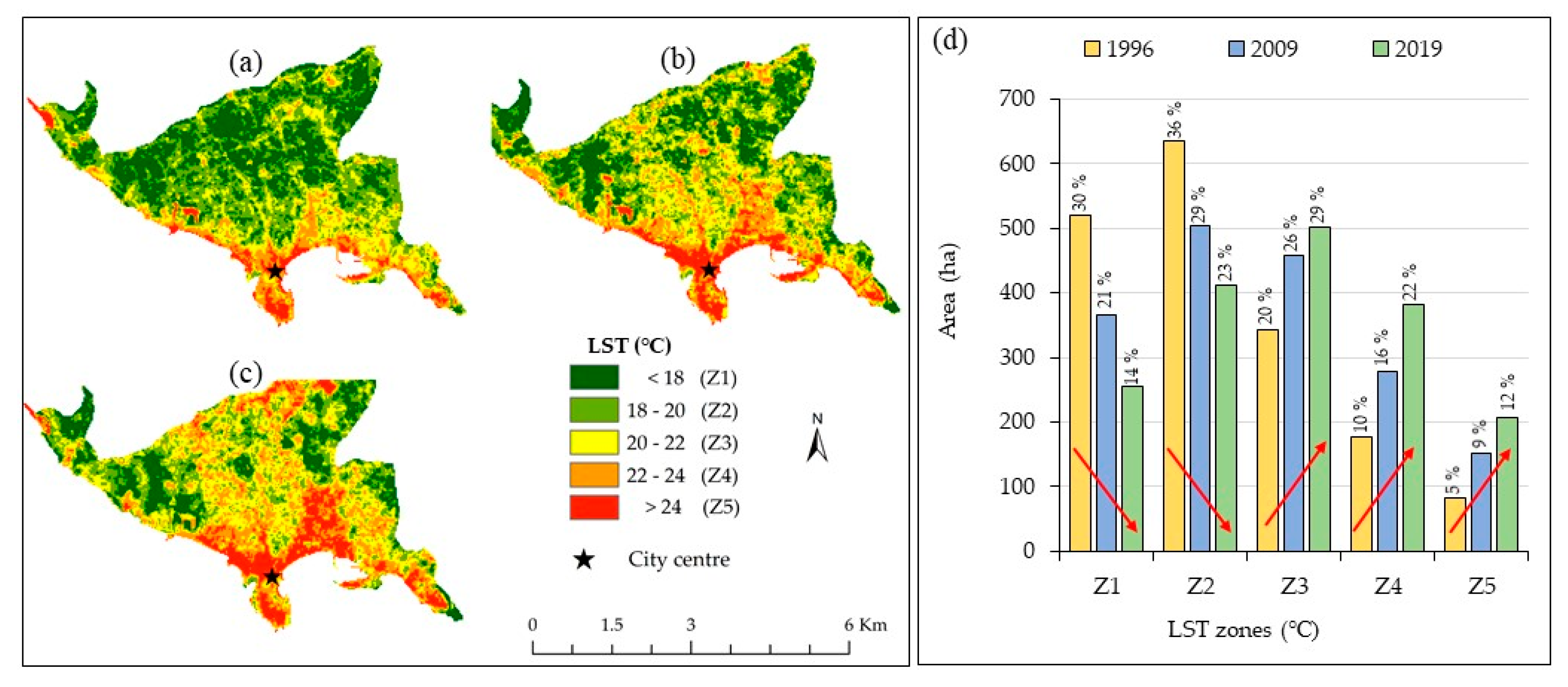
The spatiotemporal distribution of LST in 1996, 2009, and 2019 of the GMCA is shown in Figure 3a–c, respectively. Numerous researchers explain (theoretically and practically) that the range of numerical values has no scientific impact other than to explain the research area in relative terms [55,56,57]. Other than this, LST zonation maps are more convenient for comparison rather than the range’s value. Hence, the range’s values of LST were divided into five zones as follows: less than 18 °C (Z1), 18~20 °C (Z2), 20~22 °C (Z3), 22~24 °C (Z4), and greater than 24 °C (Z5). The result shows that Z4 and Z5 are observed around the city center, and their spatial distribution is stronger in 2019 than the other two time points. Both Z1 and Z2 were observed by the VG on the north side, as shown in Figure 3. Z3 was mainly observed around the mixture of LULC, especially BU and VG. From the temporal viewpoint, Z1 and Z2 are gradually declined, while Z3-Z5 are gradually increased, as shown in Figure 3d. For instance, the extended area of Z1 declined from 520 ha (30%) to 254.2 ha (14%), and the Z5 increased from 83.3 (5%) to 207.4 (12%) within the investigation period (1996–2019).
3.3. LULC Transformation and Its LST Changes
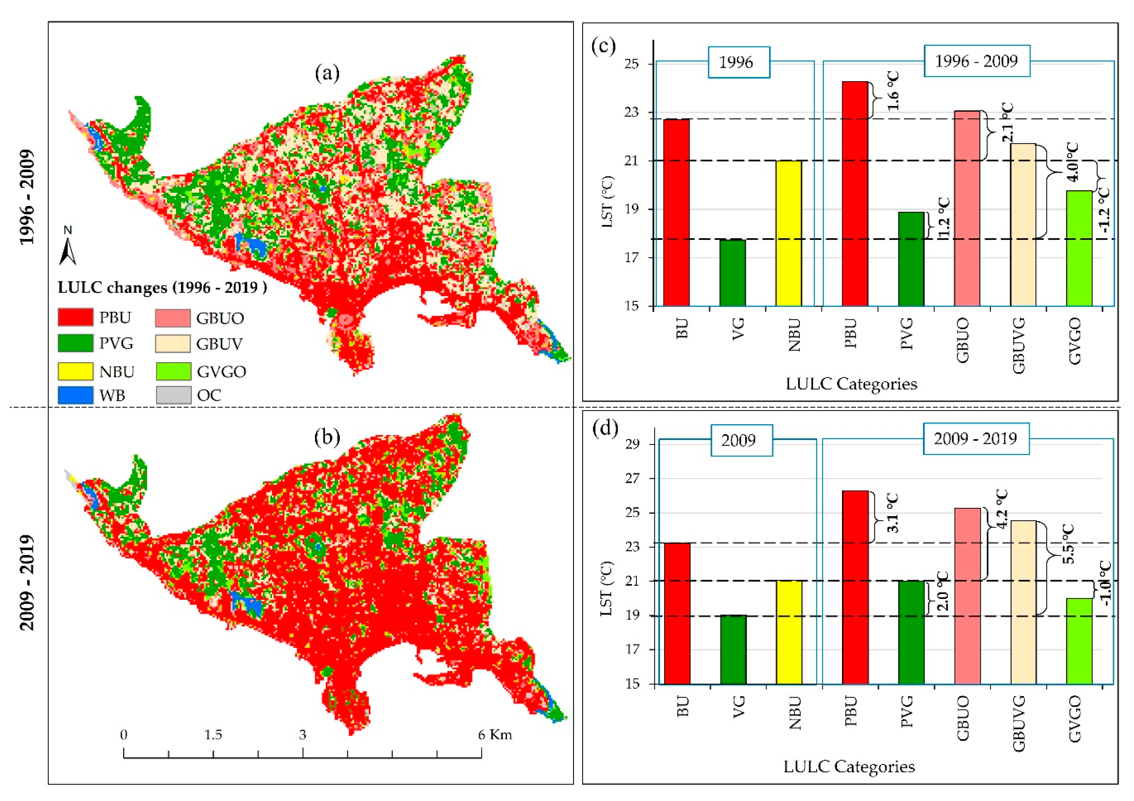
Changing of LULC is a common phenomenon in the urban expansion process, and its details can be found elsewhere [4,19,58]. The spatial distribution of resulting LULC change maps produced for 1996–2009 and 2009–2019 is illustrated in Figure 4a,d, respectively. Temporal LST variation over the changes in pairs of years, and their LST difference between before and after the change, is also illustrated in Figure 4c,d. Additionally, the same figures show the LST comparison with immediate past time point in another way of temporal variation over the decades. Meanwhile, the descriptive statistic of the changes (BU, VG) is presented in Table 2.
The rapid LST variation was observed from GBUVG, where VG was transformed to BU. In 1996, the mean LST of VG was 17.1 °C, but it increased to 21.7 °C when it transferred to BU in 2009. This emphasized that the BU area is most prominent for LST variations that the VG and its mean LST difference was 4 °C, as shown in Figure 4c. Similarly, the same change pattern was observed between 2009 and 2019; its mean LTS difference was 5.5 °C on GBUVG (Figure 4d). The BU area, which expanded by acquiring land from the NBU area, has shown a mean LST increasing trend. The mean LST of the NBU was 21 °C in 1996, but it increased to 23.1 °C after NBU change to BU. Their change difference was 2.1 °C, as shown in Figure 4c. The same trend can also be observed for GBUO in 2009–2019. Thus, the mean LST difference was 4.2 °C, as shown in Figure 4d.
Though other LULC categories show the mean LST increasing pattern, GVGO shows mean LST decreasing pattern, as shown in Figure 4c,d. It decreased by 1.2 °C and 1 °C between 1996 and 2009 and 2009 and 2019, respectively. The extended area of VG was upgraded by NBU, and it was 72.5 ha (4.2%) between 1996 and 2009, while it was 106.7 ha or 6% from 2009 to 2019 (Table 2). Mainly, the NBU area was transformed as VG in both periods. The NBU area (open land and bare land) is more prominent for reradiating, but VG lands are resistant to it. Thus, this could be the reason for the decrease in mean LST on GVGO.
LST on persistent land (PBU, PVG) increased in both investigated periods. The mean LST of the BU was 22.7 °C in 1996, and it was upgraded to 24.3 °C from 1996 to 2009, presenting a 1.6 °C difference between the two time points. A similar behavior pattern can also be seen in the VG area, and its LST difference was 1.2 °C from 1996 to 2009 (Figure 4c). There was not an exceptional case between 2009 and 2019. Its LST difference was 3.1 °C and 2.0 °C in PBU and PVG (Figure 4d), correspondingly. Even the persistent area denotes the constant land fraction, and significant LST differences were observed. If so, there should be some influence on the changes of LST on persistent land. One of the accepted reasons could be the neighboring land cover effect, as past researchers demonstrated in LST-related research [20,52].
4. Discussion
4.1. Urban Expansion and Its Influence on LST Changes
The results show that GMCA has undergone rapid LULC change in the last two decades, except WB. Because of the coastal city, a one-way city expansion pattern was observed towards the northern regions compared with others. In 1996, BU was 628.4 ha (38%), but it was upgraded to 1265.6 ha (69%) in 2009, presenting a 31% improvement (Figure 2d). However, less urban expansion (7%) was observed in 2019. This result enhances our understanding of the urbanization process in GMCA, and it may be reaching its saturated level by around 2019 [59]. However, more comprehensive research related to urban changes is required to confirm this saturation limit. As shown in Figure 2d, VG and NBU have decreased by around 26% and 12%, respectively, from 1996 to 2019. Indeed, if there are no considerable changes in WB, loose land of both VG and NBU should be captured by BU, the reason could be land demand for the expanding of social needs and industrial requirement [32]. Mean LST has increased by 4 °C (Figure 4c), and 5.5 °C (Figure 4d) on the newly added BU, which shifted from VG, in 1996–2009 and 2009–2019, respectively. As illustrated by Figure 4c,d, the mean LST on persistent land has increased. Moreover, its suggests that there is a higher possibility of increasing the overall temperature in the future. Further, LST behavior can also be imagined by examining the following key points: (i) the trends of decline on lower LST zones and incline on higher LST zones (Figure 3d); and (ii) mean LST in three-time points were observed as 19.2 °C, 20.1 °C, and 22.4 °C in 1996, 2009, and 2019, respectively. As stated above, neighboring LULC might be affected owing to LST variation in both PBU and PVG. As built-up area is made up of impermeable materials, radiation back to the atmosphere is a common phenomenon, as evidenced by past studies [4,12]. This reason might be affected by the LST variation of PBU. In 2009, vegetated land scattered as small land fractions (Figure 2c) showed a mixed land use pattern with built-up area. A mixture of land use could be the reason for increasing the LST on PVG as well [60]. However, it is noted that detailed research is required to prove how to effect neighboring and mixture of land use for the LST variation.
4.2. The Implication of the Results for Urban Development
Owing to the use of impenetrable materials (asphalt, concrete, brick, stone, and rooftops, among others), built-up area functions as a heat source in the daytime by encouraging radiation back to the atmosphere, which is known as the “heat back” phenomenon. Owing to lower thermal inertia and transpiration, the land fraction consisting of a VG generally decreases the magnitude of LST (Figure 3). Additionally, land fractions that transferred into VG from others (Figure 4c,d) showed LST deterioration trends, which could prove the power of green to control the effect of LST in an urban area. Regarding this context, city planners of GMCA can consider the concept of a green city [61,62]. Moreover, urban development strategies should be lined up with a sustainable development goal [9,63]. The previous research has proposed various kinds of greening applications for the urban area [61,62], including green walls and green roof (for low- and high-rise buildings), green zones (for the residential area), green belt (for road and riverbank), and urban agriculture [64,65].
On the basis of such information, green space can regulate the negative impact on a high temperature in an urban environment, and even a small park can make a cold surface [66]. Galle, as a tropical evergreen city, can apply these green city concepts not only for controlling LST effect, but also for enhancing its scenic beauty as a tourist interaction factor. Changing the regional climate is one of the negative impacts on LST that can affect several sections. This is most especially the case of the urban community in both residents and commuters. As noted in Section 2.1, Galle is an important tourist destination, and there are many tourist hotels in Galle City. When the temperatures increase locally, it has a direct influence on the tourist industry. Usually, travelers do not enjoy high temperatures, and the service provider must use more energy for indoor air regulator (Air conditioner machine) at hotels and in travel vehicles. Further, other economic activities and human health also can be affected by thermal discomfort [15], including heat stress and an uncomfortable living environment in working and living places.
From a regional or global aspect, making a bottleneck for urban expansion is impossible, and the elimination of the LST effect is not feasible. Thus, it is required in understanding effective mitigation and adaptation measures for urban livability [17]. One possible application is changing the method of land utilization for urban expansion. In the field investigation stage, we observed that horizontal urban development is more common than the vertical development in the GMCA. Spatiotemporal changes of LULC revealed that horizontal urban expansion had occurred by converting the NBU and VG into BU. Hence, it is necessary to encourage vertical urban development instead of horizontal to minimize unbearable LULC changes [16,19]. Additionally, low-cost natural ventilation is a suitable solution to regulate indoor air temperature in the office and settlement [67,68]. Hence, building planners can change the orientation of the new building by considering wind flow. The respective administrative bodies and city planners can use the output of this research for future planning.
4.3. Limitation of the Study
It is noted that the values of LST in each time point were dependent not only on LULC categories, but also on other biophysical attributes. It included wind speed, surface moisture, humidity, and intensity of solar radiation, which might not be temporally stable or stationary when the source satellite thermal band was captured [69]. These factors did not have a primary impact on the final results because Landsat level 2 (radiometric-calibrated and atmospheric-corrected) data were used. Further, this study attempted to analyze the spatial pattern of the LST rather than the absolute values on a temporal comparison aspect. Additionally, the total thermal budget is not the result of the daytime temperature, but also nighttime temperature [70]. However, it may not be practical to estimate nighttime LST with Landsat data. Furthermore, validation of the results is critical over large spatial and temporal scales when using satellite observations in thermal-infrared (TIR) channels [71,72], and it is a time-consuming task. Hence, I would like to note that the results might have been interpreted in light of these limitations.
5. Conclusions
This study empirically investigated the spatiotemporal charges of both LULC and LST using remote sensing data in the GMCA from 1996 to 2019. The geospatial approaches were used for examining the LULC change pattern and its influence on the variation of LST by focusing on BU and VG. The results of the research revealed that GMCA had undergone rapid urban development. Moreover, it has expanded by 31% from 1996 to 2009. However, less urban expansion has taken place in the last decade (2009–2019). VG and NBU area gradually declined, while the WB area was stable over the investigation period. The highest LST variation was observed from newly added BU, which transferred from VG. Meanwhile, the LST declining trend was observed on newly added VG.
Indeed, the results revealed that the annual mean LST increased by 3.2 °C in the last 22 years in GMCA. The results indicated that there is a higher possibility for the continuation of urban expansion. In addition, it could be affected by the existing vegetated area. So, there is an immediate need for new land transformation policies and mechanisms to mitigate the negative effect on LST for the future sustainability of urban development. The proposed method can be applied to other cities by making necessary calibration on data. Finally, we conclude that the results of this work can be used as a reference for urban planning and land use development for making an environmentally friendly, socially acceptable, and economically accountable city in GMCA.
Author Contributions
The author, D.D., proposed the topic and spearheaded the data processing and analysis, as well as the writing of the manuscript. The author has read and agreed to the published version of the manuscript.
Funding
This research received no external funding.
Acknowledgments
The authors express their gratefulness to the anonymous reviewers for their valuable comments and suggestions.
Conflicts of Interest
The author declares no conflict of interest.
Appendix A

Table A1.
Abbreviations are used in this manuscript.
| Acronyms | Meaning |
|---|---|
| LULC | Land use land cover |
| LST | Land surface temperature |
| GEE | Google Earth Engine |
| GMCA | Galle Municipal Council area |
| UNESOC | United Nations Educational Scientific and Cultural Organization |
| FR | Random forest |
| NDVI | Normalized difference vegetation index |
| BU | Built-up |
| WB | Waterbody |
| VG | Vegetation |
| NBU | Non-built-up |
| PBU | Persistence built-up |
| PVG | Persistence vegetation |
| GBUO | Gain of built-up from others |
| GBUVG | Gain of built-up from vegetation |
| GVGO | Gain of vegetation from others |
Table A2.
Properties of the Landsat images (Level 2) used in this study.
| Sensor | S. No. | Landsat ID | Acquisition Date | Time (GMT) * | Day Time Air Temperature (°C) ** |
|---|---|---|---|---|---|
| Landsat 5 (Thematic Mapper) | 1 | LT05_L1TP_141056_19960221_20170105_01_T1 | 1996-02-21 | 04:00:09 | 30.3 |
| 2 | LT05_L1TP_141056_19970223_20161231_01_T1 | 1996-02-23 | 04:19:42 | 31.0 | |
| 3 | LT05_L1TP_141056_19960324_20170105_01_T1 | 1996-03-24 | 04:02:15 | 34.7 | |
| 4 | LT05_L1TP_141056_19960425_20170105_01_T1 | 1996-04-25 | 04:04:13 | 31.3 | |
| 5 | LT05_L1TP_141056_19960527_20170104_01_T1 | 1996-05-27 | 04:06:05 | 30.2 | |
| 6 | LT05_L1TP_141056_19970530_20161231_01_T1 | 1996-05-30 | 04:23:12 | 30.8 | |
| 7 | LT05_L1TP_141056_19960714_20170104_01_T1 | 1996-07-14 | 04:08:39 | 28.1 | |
| 8 | LT05_L1TP_141056_19960730_20170103_01_T1 | 1996-07-30 | 04:09:30 | 28.7 | |
| 9 | LT05_L1TP_141056_19970717_20161231_01_T1 | 1996-07-17 | 04:24:51 | 28.5 | |
| 10 | LT05_L1TP_141056_19960815_20170103_01_T1 | 1996-08-15 | 04:10:20 | 29.0 | |
| 11 | LT05_L1TP_141056_19970802_20161230_01_T1 | 1996-08-02 | 04:25:23 | 29.2 | |
| 12 | LT05_L1TP_141056_19970919_20161229_01_T1 | 1996-09-19 | 04:26:49 | 29.4 | |
| 13 | LT05_L1TP_141056_19961002_20170103_01_T1 | 1996-10-02 | 04:12:57 | 28.9 | |
| 14 | LT05_L1TP_141056_19961119_20170101_01_T1 | 1996-11-19 | 04:15:17 | 31.2 | |
| Day time mean annual air temperature in 1996 is 30.1 °C | |||||
| Landsat 5 (Thematic Mapper) | 1 | LT05_L1TP_141056_20090107_20161028_01_T1 | 2009-01-07 | 04:39:10 | 32.5 |
| 2 | LT05_L1TP_141056_20090123_20161028_01_T1 | 2009-01-23 | 04:39:36 | 30.8 | |
| 3 | LT05_L1TP_141056_20090208_20161028_01_T1 | 2009-02-08 | 04:40:01 | 30.6 | |
| 4 | LT05_L1TP_141056_20090224_20161027_01_T1 | 2009-02-24 | 04:40:25 | 31.0 | |
| 5 | LT05_L1TP_141056_20090312_20161027_01_T1 | 2009-03-12 | 04:40:47 | 31.8 | |
| 6 | LT05_L1TP_141056_20090328_20161027_01_T1 | 2009-03-28 | 04:41:08 | 33.0 | |
| 7 | LT05_L1TP_141056_20090429_20161026_01_T1 | 2009-04-29 | 04:41:46 | 30.8 | |
| 8 | LT05_L1TP_141056_20090515_20161026_01_T1 | 2009-05-15 | 04:42:04 | 30.4 | |
| 9 | LT05_L1TP_141056_20090616_20161025_01_T1 | 2009-06-16 | 04:42:39 | 30.0 | |
| 10 | LT05_L1TP_141056_20090718_20161023_01_T1 | 2009-07-18 | 04:43:13 | 29.6 | |
| 11 | LT05_L1TP_141056_20090803_20161022_01_T1 | 2009-08-03 | 04:43:27 | 29.5 | |
| 12 | LT05_L1TP_141056_20090819_20161022_01_T1 | 2009-08-19 | 04:43:41 | 29.0 | |
| 13 | LT05_L1TP_141056_20090904_20161025_01_T1 | 2009-09-04 | 04:43:56 | 29.4 | |
| 14 | LT05_L1TP_141056_20090920_20161025_01_T1 | 2009-09-20 | 04:44:08 | 29.3 | |
| 15 | LT05_L1TP_141056_20091006_20161020_01_T1 | 2009-10-06 | 04:44:19 | 28.7 | |
| 16 | LT05_L1TP_141056_20091209_20161017_01_T1 | 2009-12-09 | 04:44:53 | 30.0 | |
| Day time mean annual air temperature in 1996 is 30.4 °C | |||||
| Landsat 8 ( Operational Land Imager and Thermal Infrared Sensor) | 1 | LC08_L1TP_141056_20190103_20190130_01_T1 | 2019-01-03 | 4:54:11 | 29.3 |
| 2 | LC08_L1TP_141056_20190220_20190220_01_T1 | 2019-02-20 | 4:54:02 | 33.5 | |
| 3 | LC08_L1TP_141056_20190308_20190324_01_T1 | 2019-03-08 | 4:53:57 | 30.3 | |
| 4 | LC08_L1TP_141056_20190324_20190403_01_T1 | 2019-03-24 | 4:53:53 | 33.1 | |
| 5 | LC08_L1TP_141056_20190409_20190422_01_T1 | 2019-04-09 | 4:53:49 | 32.1 | |
| 6 | LC08_L1TP_141056_20190511_20190521_01_T1 | 2019-05-11 | 4:53:51 | 31.0 | |
| 7 | LC08_L1TP_141056_20190527_20190605_01_T1 | 2019-05-27 | 4:54:00 | 30.8 | |
| 8 | LC08_L1TP_141056_20190612_20190619_01_T1 | 2019-06-12 | 4:54:07 | 29.4 | |
| 9 | LC08_L1TP_141056_20190628_20190706_01_T1 | 2019-06-28 | 4:54:12 | 31.0 | |
| 10 | LC08_L1TP_141056_20190714_20190719_01_T1 | 2019-07-14 | 4:54:16 | 30.5 | |
| 11 | LC08_L1TP_141056_20190730_20190801_01_T1 | 2019-07-30 | 4:54:21 | 30.0 | |
| 12 | LC08_L1TP_141056_20190831_20190916_01_T1 | 2019-08-31 | 4:54:31 | 29.1 | |
| 13 | LC08_L1TP_141056_20191002_20191018_01_T1 | 2019-10-02 | 4:54:40 | 30.9 | |
| 14 | LC08_L1TP_141056_20191018_20191029_01_T1 | 2019-10-18 | 4:54:43 | 31.7 | |
| 15 | LC08_L1TP_141056_20191103_20191115_01_T1 | 2019-11-03 | 4:54:42 | 28.7 | |
| 16 | LC08_L1TP_141056_20191119_20191202_01_T1 | 2019-11-19 | 4:54:39 | 31.6 | |
| Day time mean annual air temperature in 1996 is 30.8 °C | |||||
* Sri Lanka is 5 h and 30 min ahead of Greenwich Mean Time (GMT). ** Data source: Department of Meteorology, Sri Lanka.
References
- United Nations. UN Department of Economic and Social Affairs. The World ’s Cities in 2018; United Nations: New York, NY, USA, 2018. [Google Scholar]
- Ibrahim, G.R.F. Urban land use land cover changes and their effect on land surface temperature: Case study using Dohuk City in the Kurdistan Region of Iraq. Climate 2017, 5, 13. [Google Scholar] [CrossRef] [Green Version]
- Ranagalage, M.; Dissanayake, D.; Murayama, Y.; Zhang, X.; Estoque, R.C.; Perera, E.; Morimoto, T. Quantifying surface urban heat island formation in the world heritage tropical mountain city of Sri Lanka. ISPRS Int. J. Geo Inf. 2018, 7, 341. [Google Scholar] [CrossRef] [Green Version]
- Dissanayake, D.; Morimoto, T.; Murayama, Y.; Ranagalage, M. Impact of landscape structure on the variation of land surface temperature in Sub-Saharan Region: A case study of Addis Ababa using Landsat Data (1986–2016). Sustainability 2019, 11, 2257. [Google Scholar] [CrossRef] [Green Version]
- Rousta, I.; Sarif, M.O.; Gupta, R.D.; Olafsson, H.; Ranagalage, M.; Murayama, Y.; Zhang, H.; Mushore, T.D. Spatiotemporal analysis of land use/land cover and its effects on surface urban heat Island using landsat data: A case study of Metropolitan City Tehran (1988–2018). Sustainability 2018, 10, 4433. [Google Scholar] [CrossRef] [Green Version]
- Subasinghe, S.; Estoque, R.C.; Murayama, Y. Spatiotemporal analysis of urban growth using GIS and remote sensing: A case study of the Colombo Metropolitan Area, Sri Lanka. ISPRS Int. J. Geo Inf. 2016, 5, 197. [Google Scholar] [CrossRef] [Green Version]
- Ranagalage, M.; Wang, R.; Gunarathna, M.H.J.P.; Dissanayake, D.; Murayama, Y.; Simwanda, M. Spatial forecasting of the landscape in rapidly urbanizing hill stations of South Asia: A case study of Nuwara Eliya, Sri Lanka (1996–2037). Remote Sens. 2019, 11, 1743. [Google Scholar] [CrossRef] [Green Version]
- Priyankara, P.; Ranagalage, M.; Dissanayake, D.; Morimoto, T.; Murayama, Y. Spatial process of surface urban heat island in rapidly growing Seoul Metropolitan area for sustainable urban planning using landsat data (1996–2017). Climate 2019, 7, 110. [Google Scholar] [CrossRef] [Green Version]
- Dissanayake, D.; Morimoto, T.; Murayama, Y.; Ranagalage, M. Impact of urban surface characteristics and socio-economic variables on the spatial variation of land surface temperature in Lagos City, Nigeria. Sustainability 2019, 11, 25. [Google Scholar] [CrossRef] [Green Version]
- United Nations. UN Department of Economic and Social Affairs. World Urbanization Prospects: The 2014 Revision, Highlights; United Nations: New York, NY, USA, 2015. [Google Scholar]
- Staniec, M.; Nowak, H. The application of energy balance at the bare soil surface to predict annual soil temperature distribution. Energy Build. 2016, 127, 56–65. [Google Scholar] [CrossRef]
- Arsiso, B.K.; Mengistu Tsidu, G.; Stoffberg, G.H.; Tadesse, T. Influence of urbanization-driven land use/cover change on climate: The case of Addis Ababa, Ethiopia. Phys. Chem. Earth 2018, 105, 212–223. [Google Scholar] [CrossRef]
- EPA (Environmental Protection Agency). Reducing Urban Heat Islands: Compendium of Strategies Urban Heat Island Basics; US Environmental Protection Agency: Washington, DC, USA, 2008.
- World Health Organization. WHO Guidance to Protect Health from Climate Change through Health Adaptation Planning; WHO, Department of Public Health Environment and Social Determinants of Health: Geneva, Switzerland, 2014. [Google Scholar]
- Su, Y.F.; Foody, G.M.; Cheng, K.S. Spatial non-stationarity in the relationships between land cover and surface temperature in an urban heat island and its impacts on thermally sensitive populations. Landsc. Urban Plan. 2012, 107, 172–180. [Google Scholar] [CrossRef]
- Handayani, H.H.; Murayama, Y.; Ranagalage, M.; Liu, F.; Dissanayake, D. Geospatial analysis of horizontal and vertical urban expansion using multi-spatial resolution data: A case study of Surabaya, Indonesia. Remote Sens. 2018, 10, 1599. [Google Scholar] [CrossRef] [Green Version]
- Dissanayake, D.; Morimoto, T.; Murayama, Y.; Ranagalage, M.; Perera, E. Analysis of life quality in a tropical mountain city using a multi-criteria geospatial technique: A case study of Kandy City, Sri Lanka. Sustainability 2020, 12, 2918. [Google Scholar] [CrossRef] [Green Version]
- Ranagalage, M.; Murayama, Y.; Dissanayake, D.; Simwanda, M. The impacts of landscape changes on annual mean land surface temperature in the tropical mountain city of Sri Lanka: A case study of Nuwara Eliya (1996–2017). Sustainability 2019, 11, 5517. [Google Scholar] [CrossRef] [Green Version]
- Dissanayake, D.; Morimoto, T.; Ranagalage, M.; Murayama, Y. Land-use/land-cover changes and their impact on surface urban heat islands: Case study of Kandy City, Sri Lanka. Climate 2019, 7, 99. [Google Scholar] [CrossRef] [Green Version]
- Feng, X.; Myint, S.W. Exploring the effect of neighboring land cover pattern on land surface temperature of central building objects. Build. Environ. 2016, 95, 346–354. [Google Scholar] [CrossRef]
- Ranagalage, M.; Estoque, R.C.; Handayani, H.H.; Zhang, X.; Morimoto, T.; Tadono, T.; Murayama, Y. Relation between urban volume and land surface temperature: A comparative study of planned and traditional cities in Japan. Sustainability 2018, 10, 2366. [Google Scholar] [CrossRef] [Green Version]
- Ravanelli, R.; Nascetti, A.; Cirigliano, R.; Di Rico, C.; Leuzzi, G.; Monti, P.; Crespi, M. Monitoring the impact of land cover change on surface urban heat island through Google Earth Engine: Proposal of a global methodology, first applications and problems. Remote Sens. 2018, 10, 1488. [Google Scholar] [CrossRef] [Green Version]
- Google Erath Engine, Landsat Collection Structure. Available online: https://developers.google.com/earth-engine/landsat (accessed on 2 January 2020).
- Parastatidis, D.; Mitraka, Z.; Chrysoulakis, N.; Abrams, M. Online global land surface temperature estimation from Landsat. Remote Sens. 2017, 9, 1208. [Google Scholar] [CrossRef] [Green Version]
- Google Erath Engine, Image Collection Reductions. Available online: https://developers.google.com/earth-engine/reducers_image_collection (accessed on 2 January 2020).
- Dissanayake, D.M.S.L.B. Web GIS based spatial data infrastructure (SDI) system for forestry management in Sri Lanka. In Proceedings of the International Forestry and Environment Symposium, Negombo, Sri Lanka, 16–17 October 2015; p. 20. [Google Scholar]
- Dissanayake, D.; Morimoto, T.; Ranagalage, M. Accessing the soil erosion rate based on RUSLE model for sustainable land use management: A case study of the Kotmale watershed, Sri Lanka. Model. Earth Syst. Environ. 2018, 5, 291–306. [Google Scholar] [CrossRef]
- Hassan, Z.; Shabbir, R.; Ahmad, S.S.; Malik, A.H.; Aziz, N.; Butt, A.; Erum, S. Dynamics of land use and land cover change (LULCC) using geospatial techniques: A case study of Islamabad Pakistan. Springerplus 2016, 5, 812. [Google Scholar] [CrossRef] [PubMed] [Green Version]
- Islam, K.; Jashimuddin, M.; Nath, B.; Nath, T.K. Land use classification and change detection by using multi-temporal remotely sensed imagery: The case of Chunati wildlife sanctuary, Bangladesh. Egypt. J. Remote Sens. Sp. Sci. 2018, 21, 37–47. [Google Scholar] [CrossRef]
- Chen, X.; Zhang, Y. Impacts of urban surface characteristics on spatiotemporal pattern of land surface temperature in Kunming of China. Sustain. Cities Soc. 2017, 32, 87–99. [Google Scholar] [CrossRef] [Green Version]
- Zhou, X.; Wang, Y.C. Dynamics of land surface temperature in response to land-use/cover change. Geogr. Res. 2011, 49, 23–36. [Google Scholar] [CrossRef]
- Urban Development Authority. Development Plan for Greater Galle Area 2019–2030, Part I; Urban Development Authority: Galle, Sri Lanka, 2019.
- Abeyweera, M.A.N.S.; Kaluthanthri, P.C. Attributes of city brand of Galle City, Sri Lanka. In Proceedings of the International Conference on Real Estate Management and Valuation (ICREMV), Colombo, Sri Lanka, 21 September 2018; pp. 100–111. [Google Scholar]
- Research & International Relations Division. Annual Statistical Report 2017; Sri Lanka Tourism Development Authority: Colombo, Sri Lanka, 2018.
- Priyanwada, K.B.G.M. Women’s Status in Sri Lankan Administrative Service: A Special Reference to Galle District; Public Policy and Government Program; North South University: Dhaka, Bangladesh, 2016. [Google Scholar]
- Gorelick, N.; Hancher, M.; Dixon, M.; Ilyushchenko, S.; Thau, D.; Moore, R. Google earth engine: Planetary-scale geospatial analysis for everyone. Remote Sens. Environ. 2017, 202, 18–27. [Google Scholar] [CrossRef]
- Yu, S.; Zhu, X.; He, Q. An assessment of urban park access using house-level data in urban China: Through the lens of social equity. Int. J. Environ. Res. Public Health 2020, 17, 2349. [Google Scholar] [CrossRef] [Green Version]
- United States Geological Survey (USGS) Landsat Missions: Landsat Science Products. Available online: https://www.usgs.gov/land-resources/nli/landsat/landsat-science-products (accessed on 7 February 2019).
- Roy, A.; Inamdar, A.B. Multi-temporal Land Use Land Cover (LULC) change analysis of a dry semi-arid river basin in western India following a robust multi-sensor satellite image calibration strategy. Heliyon 2019, 5, e01478. [Google Scholar] [CrossRef] [Green Version]
- Wu, C.; Du, B.; Cui, X.; Zhang, L. A post-classification change detection method based on iterative slow feature analysis and Bayesian soft fusion. Remote Sens. Environ. 2017, 199, 241–255. [Google Scholar] [CrossRef]
- Mushore, T.D.; Dube, T.; Manjowe, M.; Gumindoga, W.; Chemura, A.; Rousta, I.; Odindi, J.; Mutanga, O. Remotely sensed retrieval of Local Climate Zones and their linkages to land surface temperature in Harare metropolitan city, Zimbabwe. Urban Clim. 2019, 27, 259–271. [Google Scholar] [CrossRef]
- Mellor, A.; Haywood, A.; Stone, C.; Jones, S. The performance of random forests in an operational setting for large area sclerophyll forest classification. Remote Sens. 2013, 5, 2838–2856. [Google Scholar] [CrossRef] [Green Version]
- Phiri, D.; Morgenroth, J. Developments in Landsat land cover classification methods: A review. Remote Sens. 2017, 9, 967. [Google Scholar] [CrossRef] [Green Version]
- Erkan, U.; Gökrem, L. A new method based on pixel density in salt and pepper noise removal. Turkish J. Electr. Eng. Comput. Sci. 2018, 26, 162–171. [Google Scholar] [CrossRef]
- Thapa, R.; Murayama, Y. Image classification techniques in mapping urban landscape: A case study of Tsukuba city using AVNIR-2 sensor data. Tsukuba Geoenvironmental. Sci. 2007, 3, 3–10. [Google Scholar]
- Sakthidasan, K.; Velmurugan Nagappan, N. Noise free image restoration using hybrid filter with adaptive genetic algorithm. Comput. Electr. Eng. 2016, 54, 382–392. [Google Scholar] [CrossRef]
- Estoque, R.C.; Murayama, Y. Monitoring surface urban heat island formation in a tropical mountain city using Landsat data (1987–2015). ISPRS J. Photogramm. Remote Sens. 2017, 133, 18–29. [Google Scholar] [CrossRef]
- Kumar, D.; Shekhar, S. Statistical analysis of land surface temperature-vegetation indexes relationship through thermal remote sensing. Ecotoxicol. Environ. Saf. 2015, 121, 39–44. [Google Scholar] [CrossRef]
- Orhan, O.; Ekercin, S.; Dadaser-Celik, F. Use of Landsat land surface temperature and vegetation indices for monitoring drought in the Salt Lake Basin Area, Turkey. Sci. World J. 2014, 2014, 142939. [Google Scholar] [CrossRef]
- Carlson, T.N.; Ripley, D.A. On the relation between NDVI, fractional vegetation cover, and leaf area index. Remote Sens. Environ. 1997, 62, 241–252. [Google Scholar] [CrossRef]
- Sobrino, J.A.; Jiménez-Muñoz, J.C.; Paolini, L. Land surface temperature retrieval from LANDSAT TM 5. Remote Sens. Environ. 2004, 90, 434–440. [Google Scholar] [CrossRef]
- Weng, Q.; Lu, D.; Schubring, J. Estimation of land surface temperature-vegetation abundance relationship for urban heat island studies. Remote Sens. Environ. 2004, 89, 467–483. [Google Scholar] [CrossRef]
- Taylor, P.; Markham, B.L.; Barker, J.L. Spectral characterization of the LANDSAT Thematic Mapper sensors. Int. J. Remote Sens. 2010, 6, 37–41. [Google Scholar]
- Estoque, R.C.; Murayama, Y.; Myint, S.W. Effects of landscape composition and pattern on land surface temperature: An urban heat island study in the megacities of Southeast Asia. Sci. Total Environ. 2017, 577, 349–359. [Google Scholar] [CrossRef]
- Nazri Che, D.; Abu Hassan, A.; Zulkiflee Abd, L.; Rodziah, I. Application of geographical information system-based analytical hierarchy process as a tool for dengue risk assessment. Asian Pac. J. Trop. Dis. 2016, 6, 928–935. [Google Scholar]
- Pawattana, C.; Tripathi, N.K. Analytical Hierarchical Process (AHP)—Based flood water retention planning in Thailand. GISci. Remote Sens. 2008, 45, 343–355. [Google Scholar] [CrossRef]
- Thirumalaivasan, D.; Karmegam, M.; Venugopal, K. AHP-DRASTIC: Software for specific aquifer vulnerability assessment using DRASTIC model and GIS. Environ. Model. Softw. 2003, 18, 645–656. [Google Scholar] [CrossRef]
- Simwanda, M.; Ranagalage, M.; Estoque, R.C.; Murayama, Y. Spatial analysis of surface urban heat Islands in four rapidly growing african cities. Remote Sens. 2019, 11, 1645. [Google Scholar] [CrossRef] [Green Version]
- Bocquier, P. World urbanization prospects: An alternative to the UN model of projection compatible with the mobility transition theory. Demogr. Res. 2005, 12, 197–236. [Google Scholar] [CrossRef]
- Su, W.; Gu, C.; Yang, G. Assessing the impact of land use/land cover on urban heat island pattern in Nanjing City, China. J. Urban Plan. Dev. 2010, 136, 365–372. [Google Scholar] [CrossRef]
- Mingaleva, Z.; Vukovic, N.; Volkova, I.; Salimova, T. Waste management in green and smart cities: A case study of Russia. Sustainability 2020, 12, 94. [Google Scholar] [CrossRef] [Green Version]
- Brilhante, O.; Klaas, J. Green City Concept and a Method to Measure Green City Performance over Time Applied to Fifty Cities Globally: Influence of GDP, Population Size and Energy Efficiency. Sustainability 2018, 10, 2031. [Google Scholar] [CrossRef] [Green Version]
- United Nations. Transforming Our World: The 2030 Agenda for Sustainable Development; United Nations General Assembly: New York, NY, USA, 2015; Volume 16301, pp. 1–35. [Google Scholar]
- Yokohari, M.; Brown, R.D.; Kato, Y.; Yamamoto, S. The cooling effect of paddy fields on summertime air temperature in residential Tokyo, Japan. Landsc. Urban Plan. 2001, 53, 17–27. [Google Scholar] [CrossRef]
- Yokohari, M.; Brown, R.D.; Kato, Y.; Moriyama, H. Effects of paddy fields on summertime air and surface temperatures in urban fringe areas of Tokyo, Japan. Landsc. Urban Plan. 1997, 38, 1–11. [Google Scholar] [CrossRef]
- Cao, X.; Onishi, A.; Chen, J.; Imura, H. Quantifying the cool island intensity of urban parks using ASTER and IKONOS data. Landsc. Urban Plan. 2010, 96, 224–231. [Google Scholar] [CrossRef]
- Abdullah, H.K.; Alibaba, H.Z. Window design of naturally ventilated offices in the mediterranean climate in terms of CO2 and thermal comfort performance. Sustainability 2020, 12, 473. [Google Scholar] [CrossRef] [Green Version]
- Chen, Y.; Tong, Z.; Malkawi, A. Investigating natural ventilation potentials across the globe: Regional and climatic variations. Build. Environ. 2017, 122, 386–396. [Google Scholar] [CrossRef]
- Ranagalage, M.; Estoque, R.C.; Zhang, X.; Murayama, Y. Spatial changes of urban heat island formation in the Colombo District, Sri Lanka: Implications for sustainability planning. Sustainability 2018, 10, 1367. [Google Scholar] [CrossRef] [Green Version]
- Shen, X.; Liu, B.; Jiang, M.; Lu, X. Marshland loss warms local land surface temperature in China. Geophys. Res. Lett. 2020, 47. [Google Scholar] [CrossRef] [Green Version]
- Tang, B.H.; Shao, K.; Li, Z.L.; Wu, H.; Nerry, F.; Zhou, G. Estimation and validation of land surface temperatures from chinese second-generation polar-orbit FY-3A VIRR data. Remote Sens. 2015, 7, 3250–3273. [Google Scholar] [CrossRef] [Green Version]
- Sobrino, J.A.; Raissouni, N.; Li, Z.L. A comparative study of land surface emissivity retrieval from NOAA data. Remote Sens. Environ. 2001, 75, 256–266. [Google Scholar] [CrossRef]
Figure 1.
Study area: (a) South Asia, (b) Sri Lanka, and (c) study area represented with a Google Earth Image (access date on 10 March 2020).
Figure 1.
Study area: (a) South Asia, (b) Sri Lanka, and (c) study area represented with a Google Earth Image (access date on 10 March 2020).

Figure 2.
Land use and land cover (LULC) map of the Galle Municipal Council area (GMCA): (a) LULC in 1996, (b) LULC in 2009, (c) LULC in 2019, and (d) temporal changes of LULC from 1996 to 2019.
Figure 2.
Land use and land cover (LULC) map of the Galle Municipal Council area (GMCA): (a) LULC in 1996, (b) LULC in 2009, (c) LULC in 2019, and (d) temporal changes of LULC from 1996 to 2019.

Figure 3.
Land surface temperature (LST) map of GMC area: (a) LST in 1996, (b) LST in 2009, (c) LST in 2019, and (d) spatiotemporal variation of LST by zones.
Figure 3.
Land surface temperature (LST) map of GMC area: (a) LST in 1996, (b) LST in 2009, (c) LST in 2019, and (d) spatiotemporal variation of LST by zones.

Figure 4.
LST variation and its different contribution by LULC categories: (a) LULC changes from 1996 to 2009, (b) LULC changes from 2009 to 2019, (c) LST variations on changes land from 1996 to 2009 and its temporal comparison with 1996, and (d) LST variations on changes land from 2009 to 2019 and its temporal comparison with 2009. PBU, persistent built-up; PVG, persistent vegetation; NBU, non-built-up; WB, waterbody; GBUO, gain of built-up from others; GBUVG, gain of built-up from vegetation; GVGO, gain of vegetation from others; OC, other changes; BU, built-up; VG, vegetation.

Table 1.
Description of land use land cover (LULC) types and their codes.
| LULC Types | Description | Code |
|---|---|---|
| Built-up | The anthropogenic or built environment, including residential, industrial, commercial, local streets, roads, and other urban areas. | BU |
| Waterbody | Areas covered by freshwater (river and ponds) and brackish water (River mouth of Gin Ganga). | WB |
| Vegetation | All types of vegetated or greenest land, including forest, agriculture, shrubs, and parks. | VG |
| Non-built-up | Rest of all LULC types that are not covered by the above three categories. | NBU |
Table 2.
Changes of BU and VG lands from 1996 to 2019 in the Galle Municipal Council (GMC) area. LST, land surface temperature; PBU, persistent built-up; PVG, persistent vegetation; GBUO, gain of built-up from others; GBUVG, gain of built-up from vegetation; GVGO, gain of vegetation from others.
Table 2.
Changes of BU and VG lands from 1996 to 2019 in the Galle Municipal Council (GMC) area. LST, land surface temperature; PBU, persistent built-up; PVG, persistent vegetation; GBUO, gain of built-up from others; GBUVG, gain of built-up from vegetation; GVGO, gain of vegetation from others.
| Investigated LULC Categories * | 1996−2009 | LST (°C) 2009 | 2009−2019 | LST (°C) 2019 | ||
|---|---|---|---|---|---|---|
| Area (ha) | Percentage | Area (ha) | Percentage | |||
| PBU | 628.4 | 38.9 | 24.3 | 1265.6 | 71.6 | 26.3 |
| PVG | 379.8 | 22.1 | 18.9 | 268.7 | 15.2 | 21.0 |
| GBUO | 216.6 | 12.6 | 23.1 | 47.7 | 2.7 | 25.3 |
| GBUVG | 420.6 | 24.5 | 21.7 | 78.3 | 4.4 | 24.5 |
| GVGO | 72.5 | 4.2 | 19.8 | 106.7 | 6.0 | 20.0 |
* Only five types of LULC change categories, derived by the post-classification change detection method (Section 2.6).
© 2020 by the author. Licensee MDPI, Basel, Switzerland. This article is an open access article distributed under the terms and conditions of the Creative Commons Attribution (CC BY) license (http://creativecommons.org/licenses/by/4.0/).
Share and Cite
MDPI and ACS Style
Dissanayake, D. Land Use Change and Its Impacts on Land Surface Temperature in Galle City, Sri Lanka. Climate 2020, 8, 65. https://0-doi-org.brum.beds.ac.uk/10.3390/cli8050065
AMA Style
Dissanayake D. Land Use Change and Its Impacts on Land Surface Temperature in Galle City, Sri Lanka. Climate. 2020; 8(5):65. https://0-doi-org.brum.beds.ac.uk/10.3390/cli8050065
Chicago/Turabian StyleDissanayake, DMSLB. 2020. "Land Use Change and Its Impacts on Land Surface Temperature in Galle City, Sri Lanka" Climate 8, no. 5: 65. https://0-doi-org.brum.beds.ac.uk/10.3390/cli8050065
Note that from the first issue of 2016, this journal uses article numbers instead of page numbers. See further details here.