1. Introduction
“How do cities form over time?” This key question posited by Herold
et al. [
1] remains unanswered in urban growth theory. The theoretical framework of urban growth as developed in [
1] and based on empirical observation, states that urban growth follows a two phase process of spatial growth: diffusion followed by coalescence and eventually, in the presence of continuous growth, saturation. Urban growth can occur at different scales: as one area reaches saturation it may become the seed of another area, and the cycle may thus repeat itself at a larger scale. The direction of growth is influenced by local factors such as topography, transportation infrastructures and planning efforts [
1], and thus urban form can evolve from and into a multitude of patterns that range from highly dispersed to highly compact [
1,
2,
3,
4,
5,
6,
7].
Sprawl is a general term that has been linked to a kind of spatial growth that occurs in regions which are neither dispersed nor compact. Although this concept has been widely discussed over the last decades, there is still no generally accepted definition [
2,
3,
4,
5,
6,
7]. For example, the same term is associated with patterns, processes, causes and consequences [
3]. On the other hand, there is a general consensus that sprawl is “
characterized by unplanned and uneven pattern of growth driven by a multitude of processes and leading to inefficient resource utilization” [
2].
Nevertheless, the existence of planning agencies, regulations and policies, does not necessarily imply more efficient resource utilization in urban areas, irrespective of whether they are located in more compact or dispersed territories. It will in fact depend on the space-time context of urban areas, something that varies among country regions and more so among different countries. Cultural, social, political, economic and physical constraints influence different time paths and contexts which may have a different impact on the resulting urban areas, even when planning regulations share some common features (whether these take the form of European legislation that must be transposed, in some sectors, to the national level, or some shared guidelines or strategies as it is the case of the countries in the European Union).
Therefore, in this study we explore the wide range of spatial structural patterns that arise in urban areas (from very dispersed to very compact) and, employing a previously developed model [
8] [based on local fractal dimension and on a Generalized Local Spatial Entropy (GLSE) function on 1 km
2 cells], establish a relation between these patterns and the set of social, economic and political changes that have taken place in NMAL - Northern Margin of the Metropolitan Area of Lisbon (and Portugal), during the last 40 years.
Fractal analysis allows us to gain insight on the morphology and spatial organization of urban areas on different scales [
4]. A significant amount of work has been developed to link fractal dimension (
D) to the morphology of cities or parts of cities [
4,
5,
8,
9,
10,
11,
12,
14] and also to establish comparisons between different cities or metropolitan areas [
11,
12,
14].
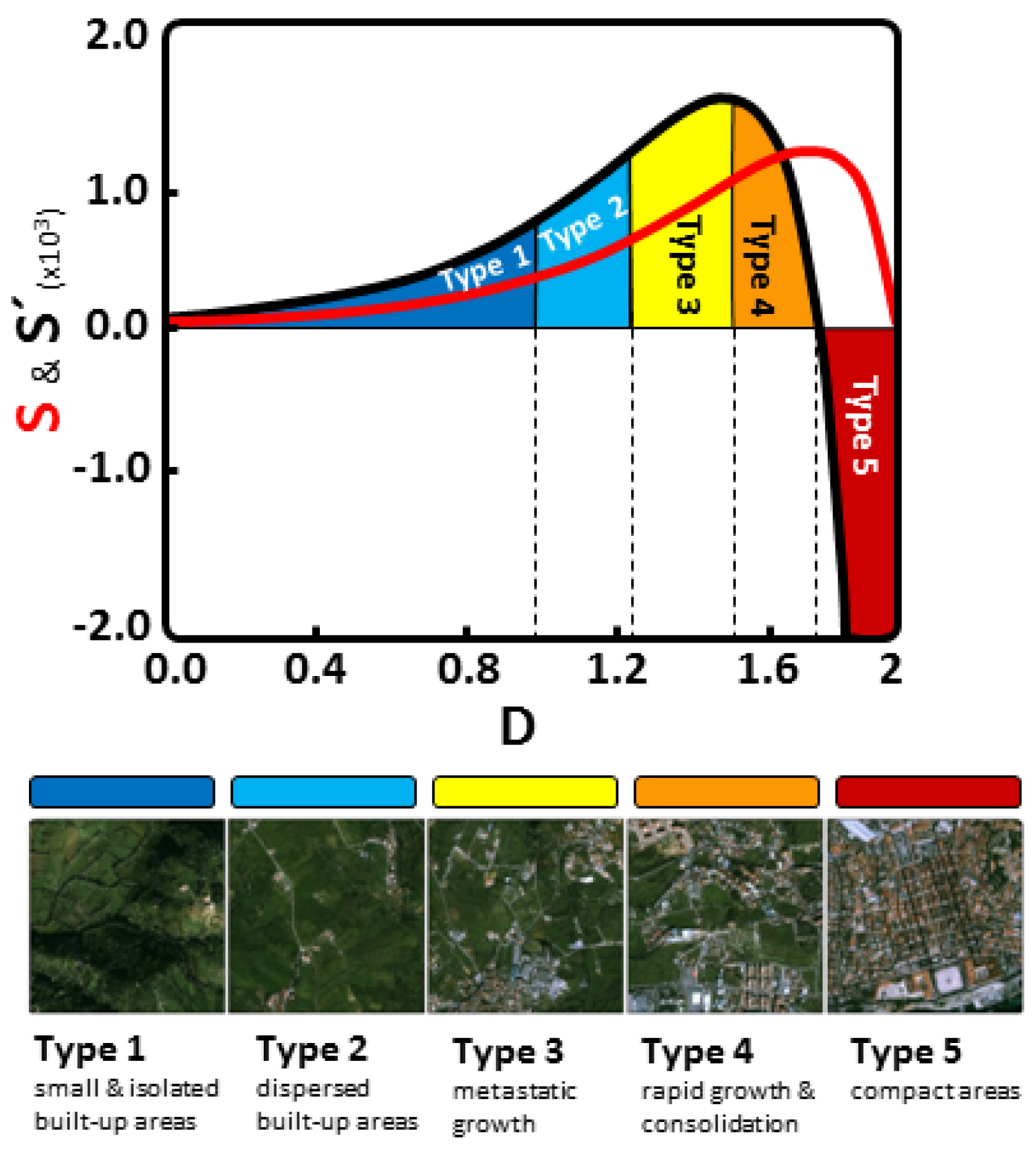
In two dimensions, D ranges from 0 to 2. Generally, lower fractal dimensions typically represent dispersed built-up areas, whereas fractal dimensions close to two are associated with compact built-up areas [
8,
13,
14]. Each built-up environment may be composed of different spatial patterns that reflect the multiple factors involved in its development and growth (topographic, cultural, aesthetic, economic, planning traditions and regulations,
etc.) as well as in its context in time. Hence, one expects to find a plethora of fractal dimensions instead of a single one. By translating the multiple fractal dimensions into five, time invariant types of patterns, we are able to characterize, in principle, any given area and, to the extent that we have longitudinal information on this area, we are also able to characterize the main changes and transformations that have taken place. Here, we apply this methodology to NMAL and characterize its development over the last forty years. Although a five year data interval would be ideal for the present analysis the available data is limited to three snapshots in time (1960, 1990 and 2004).
3. Types of Growth in NMAL
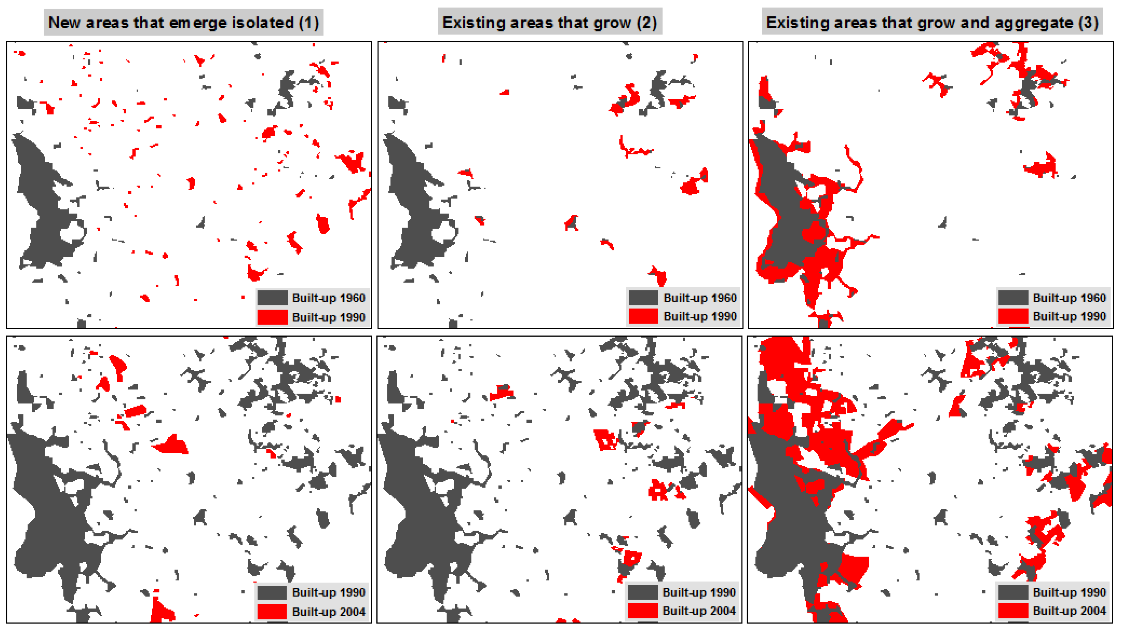
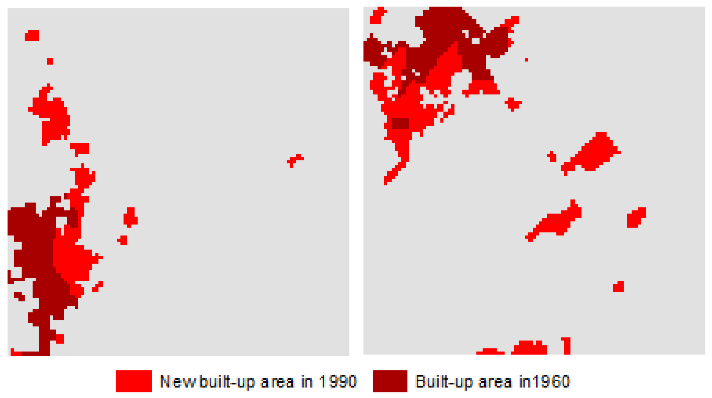
The above two growth stages can be identified by the way patches of built-up area change. Thus and for NMAL we can understand them in terms of three core growth-types: (1) new areas that emerge isolated in unoccupied sites; (2) existing areas that grew contiguously, and (3) existing areas that grew and aggregated with one or more neighboring areas (
Figure 3).
Figure 3.
Examples of growth types in NMAL.
Figure 3.
Examples of growth types in NMAL.
The examples in
Figure 3 suggest sprawl as a process, as defended in [
15,
16],
i.e., some of the linear branches of the main nucleus (see box 3 of
Figure 3), which between 1960 and 1990 could be considered sprawled areas, later became (1990–2004) compact and contiguous areas of that same nucleus. More examples of this type of transition can be found in NMAL, which clarifies the critic to references [
15,
16] made in [
3] stating that “
there is little in the literature to indicate when sprawl metamorphoses into nonsprawl”.
Overall, and in the first time period (1960–1990), the fragmentation process is visible in the 11,102 new patches that have emerged in NMAL, accounting for 80.6% of the total number of patches in 1990, but only for 16.3% of the total built-up area of the same year (see
Table 1).
The consolidation process on the other hand is confirmed by:
- (a)
286.2% growth in built-up area in existing patches (growth-type 2).
- (b)
The decrease in the number of patches (−78.3%) by growth-type 3 (growth and aggregation), but with a 167.5% increase in built-up area.
The second time period (1990–2004) was mainly dominated by the consolidation process, whether by growth-type 2 (growth) or growth-type 3 (growth and aggregation) as seen by:
- (a)
56.3% growth in built-up area in existing patches (growth-type 2).
- (b)
The decrease in the number of patches (−78.8%) in growth-type 3 but with an increase in built-up area by 44.6%.
- (c)
The number of new patches that have emerged (accounting for only 11% of total patches in 2004), that show a much weaker fragmentation process.
These dynamics reflect a metropolitan model that, in the course of time, shifted from monocentric to polycentric due to a set of socio, political and economic changes (the end of the dictatorship in 1974, the inclusion into the European Union in 1986, banking privatization, generalized higher income, access to credit, higher foreign investment,
etc.) [
17,
18], and changes in the mobility patterns, with the decrease in the share of public transport in daily travels as opposed to the increase in individual transport [
19].
However, and despite the transfer of people, industry and commercial activities to the suburbs [
17] these continued to grow in terms of built-up area in a way that surpassed the real necessities. Between 1960 and 2006, the NMAL witnessed an increase by 60.3% in population, a value quite far from the 247.1% and 202.8% increase in buildings and lodgings, respectively [
20].
The different growth-types identified in NMAL are also reflected in the proportion of the total number of patches and built-up area of each region type (see
Table 2). As expected, the number of patches is higher in less compact regions types (1, 2 and 3) and the built-up area is higher in region types 4 and 5.
Due to the fragmentation that characterized the first time period, the highest percentage of patches in NMAL changed from type 1, in 1960, to type 3 in 1990 and 2004. However, the proportion of type 3 built-up area registered a continuous decrease in all three moments (in the same way as types 1 and 2), which indicates the transition into the second growth stage where consolidation by compactification dominates, as shown by the behavior of types 4 and 5.
Table 1.
Types of growth in NMAL *.
Table 1.
Types of growth in NMAL *.
| 1960–1990 | N.° of patches | % | % of change | Built-up (m2—millions) | % | % of change |
|---|
| 1960 | 1990 | 1960 | 1990 | 1960 | 1990 | 1960 | 1990 |
|---|
| No change | 459 | 459 | 9.9 | 3.3 | 0.0 | 0.5 | 0.5 | 1.1 | 0.3 | 0.0 |
| New patches (1) | − | 11,102 | − | 80.6 | − | − | 26.7 | − | 16.3 | − |
| Growth (2) | 1666 | 1666 | 36.1 | 12.1 | 0.0 | 4.1 | 15.7 | 8.2 | 9.6 | 286.2 |
| (4.6) |
| Growth & Aggregation (3) | 2497 | 542 | 54.0 | 3.9 | −78.3 | 45.2 | 120.8 | 90.7 | 73.8 | 167.5 |
| (−5.0) | (3.3) |
| Total | 4622 | 13,769 | 100 | 100 | 197.9 | 49.8 | 163.8 | 100 | 100 | 229.1 |
| (3.7) | (4.1) |
| 1990–2004 | N. ° of patches | % | % of change | Built-up (m2—millions) | % | % of change |
| 1990 | 2004 | 1990 | 2004 | 1990 | 2004 | 1990 | 2004 |
| No change | 9432 | 9432 | 68.5 | 73.5 | 0.0 | 16.0 | 16.0 | 9.8 | 6.8 | 0.0 |
| New patches (1) | − | 1406 | − | 11.0 | − | − | 6.0 | − | 2.5 | − |
| Growth (2) | 1367 | 1367 | 9.9 | 10.7 | 0.0 | 14.0 | 21.9 | 8.6 | 9.2 | 56.3 |
| (3.2) |
| Growth & Aggregation (3) | 2970 | 629 | 21.6 | 4.9 | −78.8 | 133.7 | 193.4 | 81.7 | 81.5 | 44.6 |
| (−10.5) | (2.7) |
| Total | 13,769 | 12,834 | 100 | 100 | −6.8 | 163.8 | 237.4 | 100 | 100 | 44.9 |
| (−0.5) | (2.7) |
Table 2.
Number of patches and built-up area, by types (%).
Table 2.
Number of patches and built-up area, by types (%).
| Types | % N.º patches | % of Built-up area |
|---|
| 1960 | 1990 | 2004 | 1960 | 1990 | 2004 |
|---|
| 1 | 32.7 | 10.7 | 7.9 | 4.2 | 1.2 | 0.6 |
| 2 | 32.3 | 29.4 | 18.0 | 11.1 | 7.0 | 2.9 |
| 3 | 25.9 | 38.4 | 41.9 | 25.7 | 20.5 | 15.7 |
| 4 | 7.3 | 19.2 | 28.9 | 24.8 | 37.7 | 33.0 |
| 5 | 1.8 | 2.4 | 6.4 | 34.2 | 33.6 | 47.8 |
| Total | 100 | 100 | 100 | 100 | 100 | 100 |
The Planning System...Neither Just in Case, Nor Just in Time
The self-organization component identified in NMAL [
8] was not unfamiliar to the central administration and several plans and laws were designed to rectify and control these dynamics, after decades with few approved plans. In fact, until 1960 the only Regional Plan that existed in NMAL was the Urbanization Plan of
Costa do Sol (approved in 1948), but it only covered the coastal strip of Lisbon, Oeiras and Cascais municipalities (the southern part of the area under study).
After 1960, several planning landmarks could be enumerated:
- (a)
The first regional plan for the entire Metropolitan Area of Lisbon was the Plano Director de Desenvolvimento Urbanístico da Região de Lisboa - PDRL (Regional Master Plan). Its scope was defined by a new diploma in 1959, but it was never approved.
- (b)
The non-approval of the PDRL weakened the idea of a regional strategy for urban growth [
21] in that the administration limited itself to the evaluation and approval of allotment projects. Without the necessary planning instruments, suburbanization grew “
without any supervision and guidance, boosted by improving accessibility and increasing rates of motorization, thus sharpening their effects within” [
21].
- (c)
Parallel to the non-approval of the PDRL, a new law was published in 1965 which enabled the participation of the private sector in the urban allotment processes. By enabling allotment processes in not only urban areas but also in rural areas it triggered the sprawl of built-up areas throughout Lisbon peripheries. Without a regional strategic plan that could orient their co-development, these areas grew based mainly on the strategies of housing market agents that sought profit maximization in the process of land conversion.
- (d)
In 1976, Law No. 794/76 (Lei dos Solos), still in effect today, aimed at avoiding urban speculation and to solve the housing shortage problem. Although ambitious in some measures, as for example the delineation of areas aimed to control future land use changes near urban centers, it was never fully enforced.
- (e)
In 1982, the Municipal Master Plan (Plano Director Municipal—PDM) was enacted, which would encompass and regulate, through zoning regulations, the entire territory of a municipality (previously only urban areas would have been the object of any kind of an urbanization plan).
- (f)
However, before 1990 few municipalities in Portugal had their Master Plans approved. But the scenario changed when in that same year, Law No. 69/90 made them mandatory. Simultaneously, a municipality could not apply to European funds without an approved Master Plan. Following the general national trend, several Master Plans were approved for NMAL between 1993 and 1999. By 2000, the Metropolitan Area of Lisbon was finally covered by municipal plans although with little or no interrelationship among them, not even between neighboring municipalities.
- (g)
In 1992, a new Regional Plan was developed but again not approved, as a result of political decisions. It was only in 2002 that a Regional Plan for the Metropolitan Area of Lisbon (
PROTAML) was approved. In its strategic vision, the plan included several scales within MAL and between MAL and the national context [
22].
The above landmarks of the Portuguese planning system show that the several planning instruments actually just established existing dynamics and few or even none had the capacity to change those same dynamics into more suitable paths (as for example by mitigating the growth of a disconnected urban metropolis). Urban growth thus seems to have been more conducted by processes than by plans.
In [
23] Alfasi and Portugali argued that the traditional
just-in-case planning approach should be replaced by
just-in-time planning. The first is structured from a hierarchical top-down perspective and aims to pre-determine the future needs of a given territory. The second tries to adapt to the self-organization nature of cities. Within this approach
“a city does not have any future complete picture in the form of a long-term plan that it should accomplish” [
23]. Planning rules and instruments should be flexible enough to adapt to present and short-term future needs, as well as to change according to the location context in which they have to be applied.
The planning system in Portugal and specifically that of NMAL cannot be fully characterized by any of these approaches. The opportunity to implement a just-in-time planning system was lost when, in the presence of pre-existing self-organized dynamics, the central and local administrations adopted a generalized one-fit-all paradigm. In turn, the just-in-case approach was late and weak in controlling undesirable paths and in delineating a regional strategic vision.
One example of the failure of the
just-in-case approach is given, paradoxically, by the Municipal Master Plans. This plan established new regulations for the spatial layout of land uses (zoning) of a given territory and defined the rules of where and how new development areas could occur. These new development areas would define the urban perimeters, together with existing urban areas, equipment and infrastructures,
etc. Hence, and in theory, one could expect a greater control on the fragmentation and dispersion processes. However, in practice
“there was an over sizing of the land under urban and urbanized categories, with spaces classified for urban use in excess in terms of urbanization needs” [
18]. In the end, we can say that this normative
just-in-case planning system acted against it-self by triggering deviations to what it was trying to control as, for example, urban speculation.
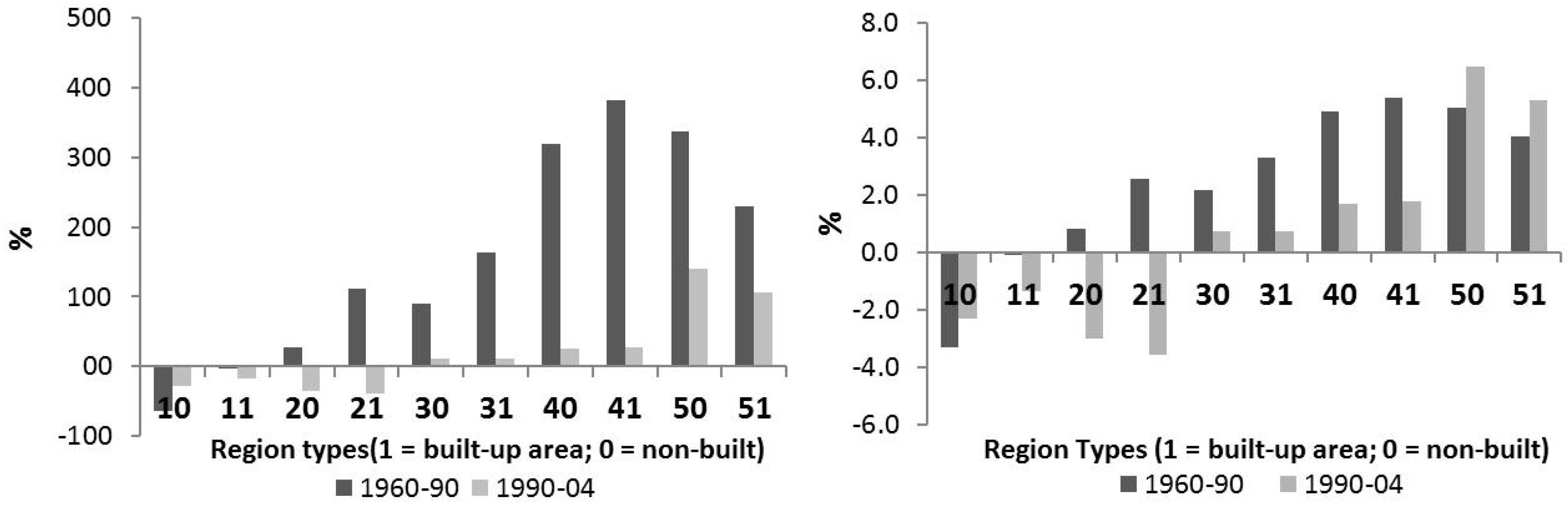
4. Spatial Transitions among Region Types
In order to understand the kind of changes that have occurred in NMAL during the two time periods, we have discretized our region types in two categories: built-up areas (1) and non-built areas (0). For example, an area coded as “50” will correspond to non-built of region type 5.
Figure 4 depicts the same information as
Figure 2, taking now this break-up into consideration. The transitions between non-built and built-up areas, among region types, are given in
Table 3 and
Table 4. The convention used (since our model of region types was constructed based on built-up areas) was that a given cell will change from Type
a to Type
b if and only if, there is any change from non-built to built-up areas and if this growth is large enough to trigger the change in cell type. Otherwise, that cell will retain its type. On the other hand, if a cell changes type, then all non-built and pre-existing built-up areas of that same cell will also change type. As a result, the only “true” changes in land cover (
Table 3 and
Table 4) are those in the grey area (lower left quadrant). All the other transitions are driven by those changes.
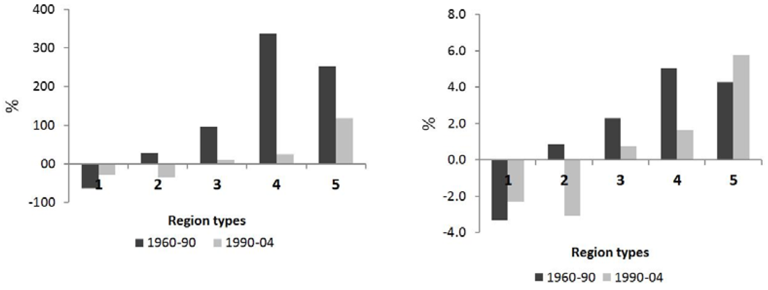
Figure 4.
Growth rates (Left) and average annual growth rates (Right), for built-up and non-built areas, by region type, 1960–1990 and 1990–2004.
Figure 4.
Growth rates (Left) and average annual growth rates (Right), for built-up and non-built areas, by region type, 1960–1990 and 1990–2004.
There are two subtle differences worth pointing out:
- (a)
Between 1960 and 1990, built-up areas in Types 2, 3 and 4 grew much more than non-built areas, as opposed to Types 1 and 5. These kinds of changes reflect mostly external transitions between region types rather than internal ones (see
Table 3).
- (b)
Between 1990 and 2004 and as NMAL entered a period of consolidation and compactification, both categories show similar growth rates, apart from Type 5 where non-built areas grew more than built-up ones, as new cells not completely developed entered this region type.
Table 3 and
Table 4 show that not only built-up areas of dispersed types can change into more compact ones (e.g. 21→31); but that the reverse is also possible (
e.g. 31→21, highlighted in red in
Table 3 and
Table 4). In this last type of transition, the increase in built-up area has contributed to a more spread, and sometimes linear, pattern (
Figure 5), thus diminishing its degree of compactness.
Reverse transitions were more prone to emerge between 1960 and 1990 than between 1990 and 2004, although they represented, respectively, only 0.60% and 0.09% of total area.
Table 3.
Transitions between 1960 and 1990 (m2—millions).
Table 3.
Transitions between 1960 and 1990 (m2—millions).
| Area m2 | 1990 | |
|---|
| 11 | 21 | 31 | 41 | 51 | 10 | 20 | 30 | 40 | 50 | Total |
|---|
| 1960 | 11 | 0.2 | 0.9 | 0.7 | 0.3 | 0.02 | | | | | | 2.1 |
| 21 | 0.01 | 0.7 | 2.9 | 1.4 | 0.4 | | | | | | 5.5 |
| 31 | | 0.1 | 3.3 | 7.8 | 1.8 | | | | | | 13.0 |
| 41 | | | 0.1 | 4.4 | 8.3 | | | | | | 12.8 |
| 51 | | | | | 16.4 | | | | | | 16.4 |
| 10 | 1.9 | 8.0 | 12.5 | 12.7 | 2.0 | 249.5 | 245.5 | 122.7 | 33.6 | 1.9 | 690.4 |
| 20 | 0.004 | 1.8 | 10.9 | 12.7 | 6.3 | 1.0 | 57.9 | 113.0 | 33.2 | 5.2 | 242.1 |
| 30 | | 0.1 | 3.6 | 19.7 | 8.1 | | 3.8 | 49.3 | 60.5 | 6.0 | 151.2 |
| 40 | | | 0.1 | 2.8 | 8.2 | | | 1.8 | 10.4 | 9.4 | 32.8 |
| 50 | | | | | 2.4 | | | | | 3.6 | 6.0 |
| Total | 2058 | 2.1 | 11.6 | 34.2 | 61.8 | 54.1 | 250.5 | 307.2 | 286.8 | 137.8 | 26.2 |
Table 4.
Transitions between 1990 and 2004 (m2—millions).
Table 4.
Transitions between 1990 and 2004 (m2—millions).
| Area m2 | 2004 | |
|---|
| 11 | 21 | 31 | 41 | 51 | 10 | 20 | 30 | 40 | 50 | Total |
|---|
| 1990 | 11 | 1.4 | 0.6 | 0.1 | 0.01 | | | | | | | 2.1 |
| 21 | | 4.6 | 6.1 | 0.8 | 0.1 | | | | | | 11.6 |
| 31 | | | 16.9 | 16.7 | 0.6 | | | | | | 34.2 |
| 41 | | | 0.1 | 30.2 | 31.6 | | | | | | 61.8 |
| 51 | | | | | 54.1 | | | | | | 54.1 |
| 10 | 0.3 | 0.8 | 1.4 | 0.7 | | 179.9 | 47.8 | 17.5 | 2.0 | | 250.5 |
| 20 | | 1.0 | 6.0 | 3.8 | 0.7 | | 152.4 | 128.2 | 14.2 | 0.8 | 307.2 |
| 30 | | | 7.2 | 16.8 | 1.7 | | | 171.2 | 87.5 | 2.2 | 286.8 |
| 40 | | | 0.01 | 10.1 | 18.1 | | | 0.9 | 70.3 | 38.3 | 137.8 |
| 50 | | | | | 4.6 | | | | | 21.6 | 26.2 |
| Total | 1.7 | 7.0 | 37.9 | 79.1 | 111.5 | 179.9 | 200.2 | 317.9 | 174.1 | 63.0 | 1172.2 |
Figure 5.
Two examples of cells that grew in built-up area but changed to a less compact type (4→3).
Figure 5.
Two examples of cells that grew in built-up area but changed to a less compact type (4→3).
At present, it is not possible to ascertain if reverse transitions should be more present in territories where generalized urban growth with fragmentation has occurred. Moreover, it is not clear if in NMAL it was more expressed before 1990 since we do not have data for intermediate time periods. However, this type of space fragmentation should be carefully acknowledged by planning agencies since it can trigger new fronts for urban development (planned or unplanned) and may contribute to the emergence of additional sprawled areas.
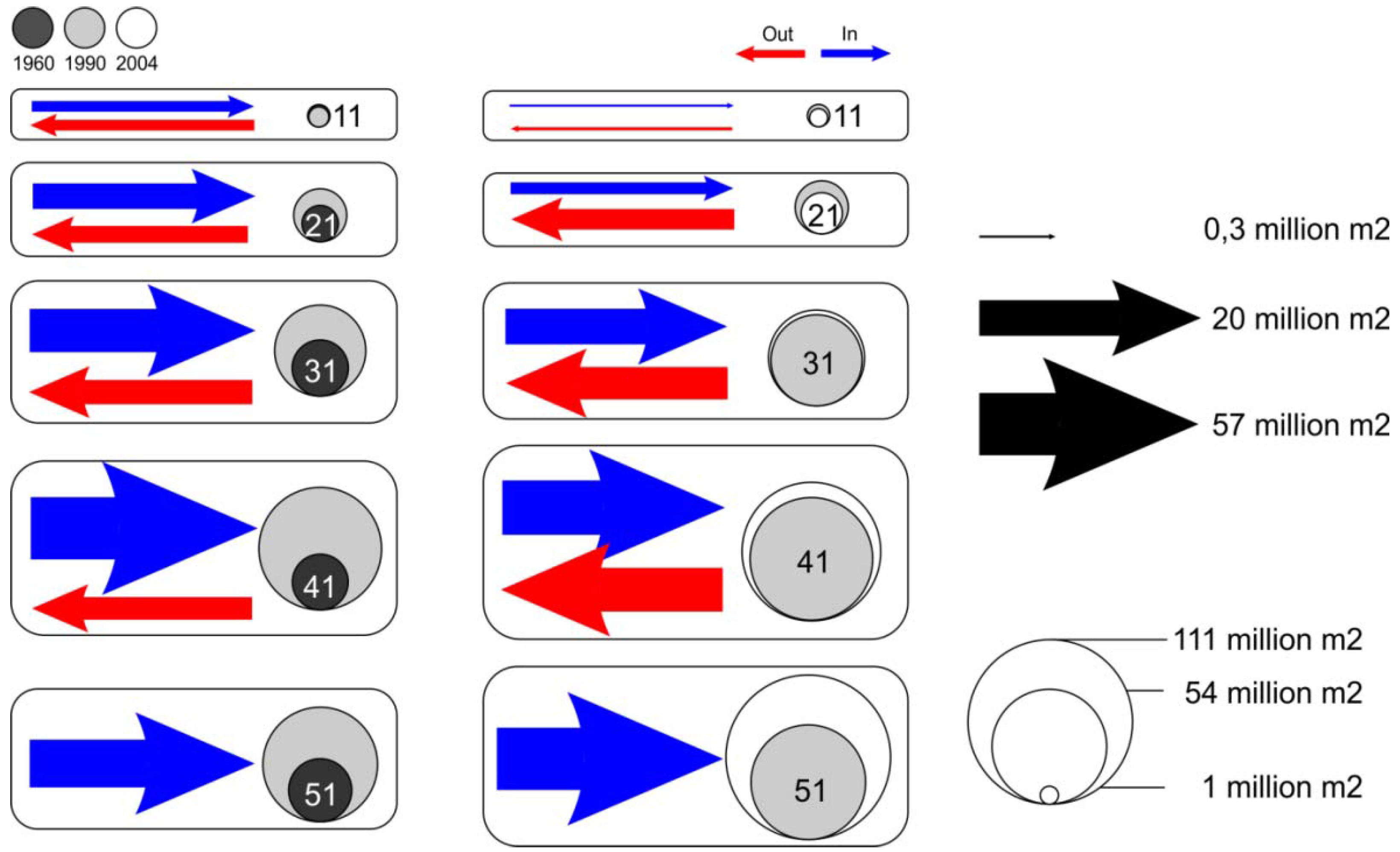
The majority of transitions occurred among types, as seen by the in and out fluxes in built-up area for each type (
Figure 6). Where out-fluxes are higher than in-fluxes, the total built-up area decreases between time periods, as was the case for Types 1 and 2.
Figure 6.
Fluxes of built-up area in each region type.
Figure 6.
Fluxes of built-up area in each region type.
All region Types (with the exception of Type 5) registered a decrease in the amount of in-fluxes in the second time period. However, only Types 3 and 4 show a positive difference between the amount of built-up area that goes in and the one that goes out. In the future, if the process of consolidation by compactification continues to shape urban growth in NMAL, then it seems probable that Type 3 will start to behave in the same way as Types 1 and 2 (i.e., decreasing its total built-up area as cells will change to more compact types). But, if fragmentation starts to emerge again then a rise is expected in the in-fluxes of Type 3, which will probably be caused also by reverse transitions.
In the presence of more self-organized urban growth, where built-up area grows without a predefined planning strategy at the metropolitan level (as it was the case of NMAL), one should expect that transitions between region types would follow in a
sequential (forward) way as seen in
Table 5 (highest percentage in each type underlined).
Table 5.
Transitions between region types in both time periods.
Table 5.
Transitions between region types in both time periods.
| 1960–1990 (%) | 1 | 2 | 3 | 4 | 5 | Total | 1990–2004 (%) | 1 | 2 | 3 | 4 | 5 | Total |
|---|
| 1 | 36.3 | 36.7 | 19.6 | 6.7 | 0.6 | 100 | 1 | 71.9 | 19.4 | 7.6 | 1.1 | | 100 |
| 2 | 0.4 | 24.4 | 51.2 | 19.1 | 4.8 | 100 | 2 | | 49.6 | 44.0 | 5.9 | 0.5 | 100 |
| 3 | | 2.4 | 34.2 | 53.7 | 9.7 | 100 | 3 | | | 60.9 | 37.7 | 1.4 | 100 |
| 4 | | | 4.4 | 38.7 | 56.9 | 100 | 4 | | | | 55.4 | 44.1 | 100 |
| 5 | | | | | 100 | 100 | 5 | | | | | 100 | 100 |
Theoretically, non-sequential (forward) transitions among types (e.g. from 2→4) should be encountered in large areas which would result from planned interventions or considerable real estate investments. However, due to a time lag of 30 and 14 years in the data, the amount of built-up area involved in this kind of transitions leads us to say (also by empirical knowledge) that the non-sequential transitions encountered here only reflect the final stage of the growth process. Nevertheless, we do acknowledge that in some specific areas real direct transitions must have occurred and that future work is needed in order to confirm this hypothesis.
In NMAL
sequential transitions arise mostly when one considers all the area in a region type,
i.e., its built and non-built area, the later always higher in proportion than the former (higher than 92% in Types 1, 2 and 3 and 71% in type 4), with the exception of Type 5 (27%). But the scenario changes slightly when one looks only at changes that have occurred from non-built (0) to built-up (1)—the grey area in
Table 3 and
Table 4 (
Table 6).
Table 6.
Transitions form non-built (0) to built-up (1) by region type.
Table 6.
Transitions form non-built (0) to built-up (1) by region type.
| 60–90 (%) | 11 | 21 | 31 | 41 | 51 | Total | 90–04 (%) | 11 | 21 | 31 | 41 | 51 | Total |
|---|
| 10 | 5.0 | 21.5 | 33.8 | 34.2 | 5.5 | 100 | 10 | 10.7 | 23.8 | 44.6 | 20.9 | | 100 |
| 20 | 0.01 | 5.8 | 34.3 | 40.0 | 19.8 | 100 | 20 | | 8.8 | 51.8 | 33.2 | 6.3 | 100 |
| 30 | | 0.2 | 11.5 | 62.6 | 25.7 | 100 | 30 | | | 28.1 | 65.2 | 6.8 | 100 |
| 40 | | | 1.0 | 25.4 | 73.6 | 100 | 40 | | | | 35.7 | 64.3 | 100 |
| 50 | | | | | 100 | 100 | 50 | | | | | 100 | 100 |
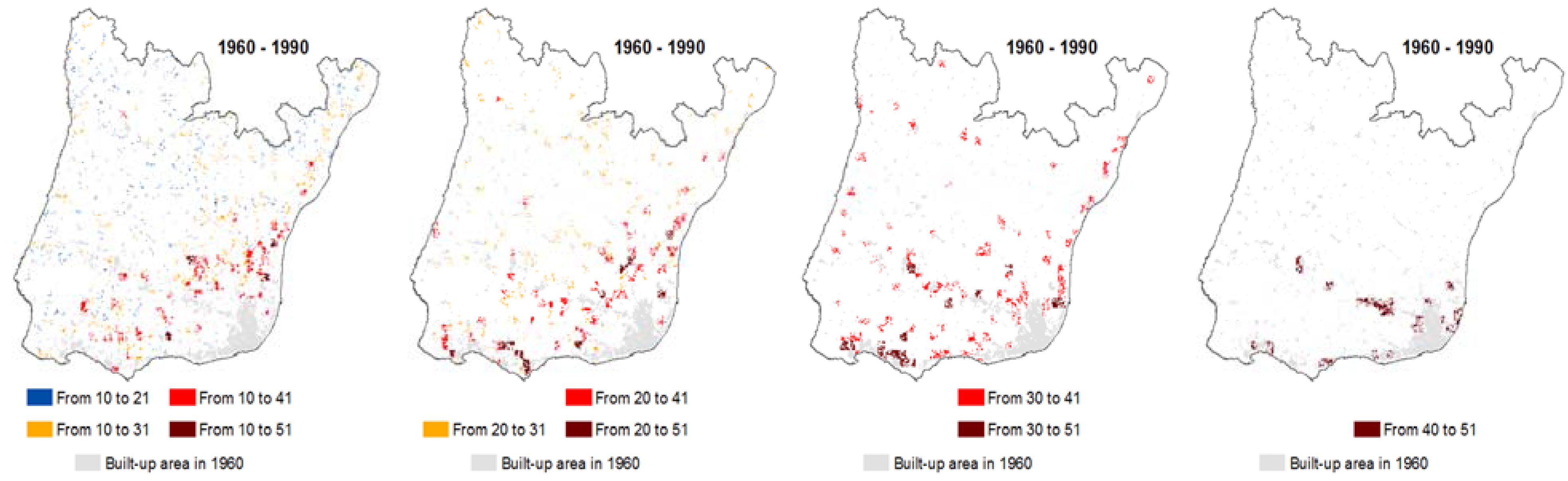
Between 1960 and 1990, Types 1, 2 and 3 show a higher percentage of change into Type 4, followed by Type 3. The spatial distribution (
Figure 7 and
Figure 8) of those changes shows that they have different roles in structuring the territory:
Between 1960 and 1990, the process of fragmentation was mainly driven by region Types 2 and 3 (
Figure 7—changes from non-built to built-up 10→21, 10→31, 20→31). But in the same time period, NMAL also registered consolidation of its pre-existing overall spatial structure, and this can be seen by looking at the changes to more compact types that have occurred in areas near Lisbon city and its suburbs (changes from 20→41, 20→51, 30→41, 30→51 and 40→51).
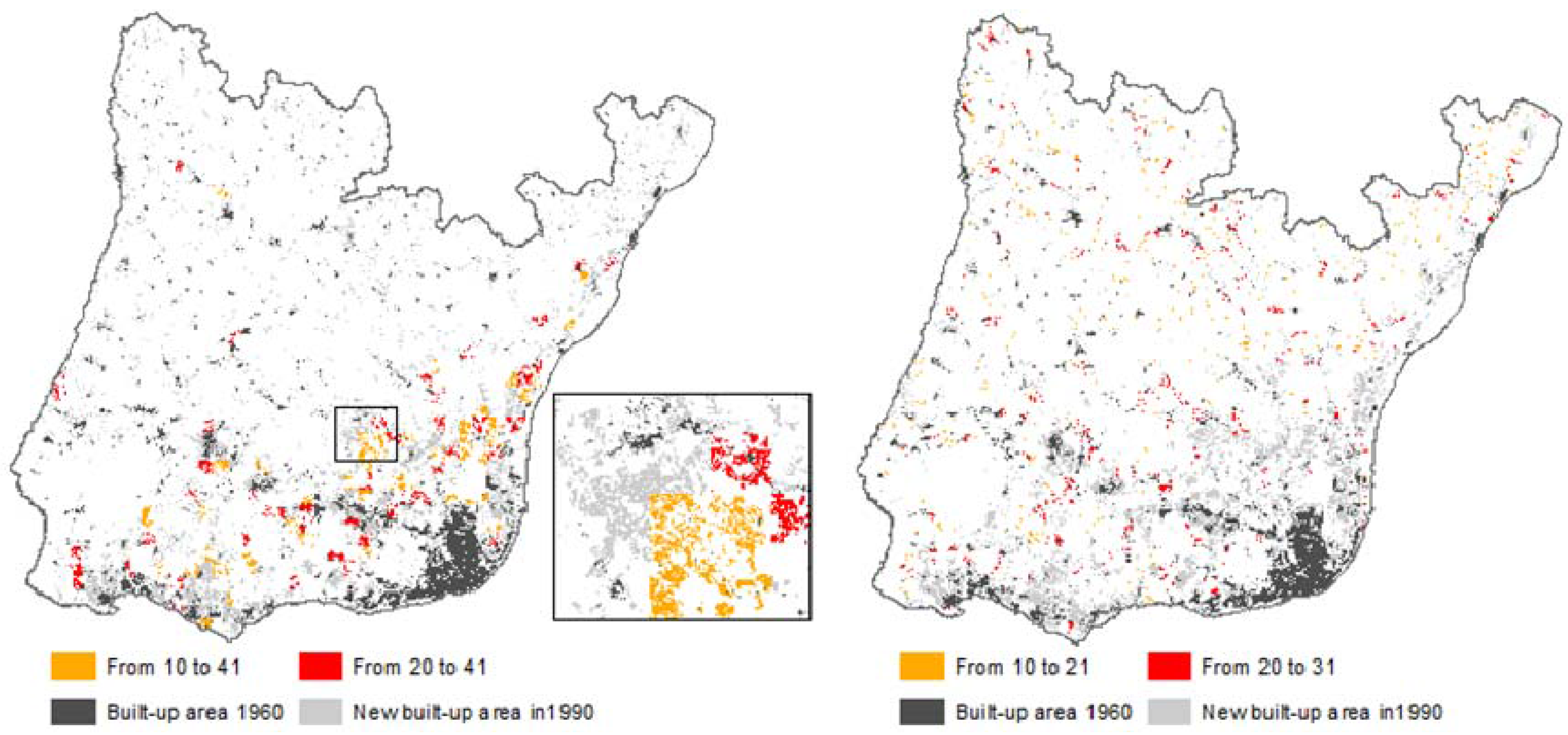
Figure 7.
Transitions from non-built to built-up areas, between region types 1960–1990.
Figure 7.
Transitions from non-built to built-up areas, between region types 1960–1990.
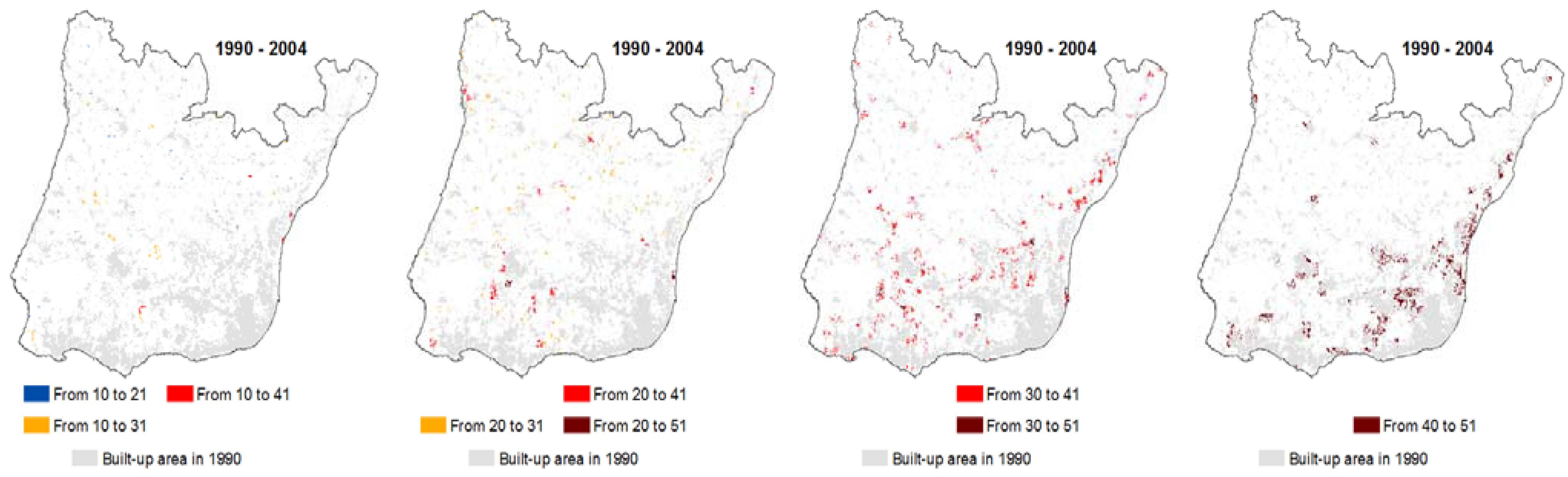
In the second time period (1990–2004) the fragmentation process did not end but it took on a residual role as seen in
Figure 8 (it was still driven by the same region types 2 and 3). Growth was characterized mainly by infill processes,
i.e., by growth and aggregation processes as previously illustrated in
Table 1, which are captured by transitions 30→41, 30→51 and 40→51.
Figure 8.
Transitions from non-built to built-up areas, between region types 1990–2004.
Figure 8.
Transitions from non-built to built-up areas, between region types 1990–2004.
These results show that although both processes of fragmentation and consolidation can occur in all region types, the latter is mainly found in more compact ones. This being said it should be noted that Type 3 played a fundamental role in both fragmentation and consolidation processes (51.3% of all possible transitions went through type 3, in at least one moment in time). It thus seems that this region type displays some hybrid behavior that connects both processes. In fact, the hybrid behavior can be understood by inspecting the features that characterize Type 3 regions: large values of
S(
D) covering a sizeable dimensional range, combined with the fastest rate of increase of
S(
D)—given by
S’(
D)—see
Figure 1. In other words, in this dimensional regime, the large values of
S(
D) and
S’(
D) pave the way for rapid transformations of built-up area, thus allowing for such a dual result, as opposed to Type 4 and Type 5 regions, where compactification is so high that one observes mostly consolidation.
Of course one way to pre-determine and rapidly change the spatial growth of built-up areas is to enforce non-sequential transitions among types (e.g., 10→41), by promoting major development projects, instead of waiting for a more “natural” growth to occur which will induce sequential transitions (e.g., 10→21). Hence, promoting non-sequential transitions would occur from a top-down approach and not from a bottom-up, self-organized one. However, we can find in NMAL, and especially between 1960 and 1990, non-sequential transitions that are not explained by direct top-down approaches.
The inset in
Figure 9 shows an area centered in a place called “Casal de Cambra”, an example of the multiple informal settlements that emerged in NMAL mostly after 1960. An informal settlement usually emerged when large parcels were sold to several owners, who in turn would subdivide them into smaller lots, through an illegal subdivision process [
24]. These lots would not have a permit to build or any type of urbanization plan. The lack of public spaces, collective equipment and infrastructures were thus a general rule and not the exception. Their emergence was enhanced by a set of interrelated factors such as the lack of affordable homes in Lisbon city, easy opportunities to gain large profits for those that sold the land, and weak local and central administrations that would often “turn a blind eye” to these dynamics, as a way to solve a problem (housing shortage) that they could not [
17,
24].
Figure 9.
Types 1 and 2 non-sequential (left) and sequential (right) transitions, 1960–1990.
Figure 9.
Types 1 and 2 non-sequential (left) and sequential (right) transitions, 1960–1990.
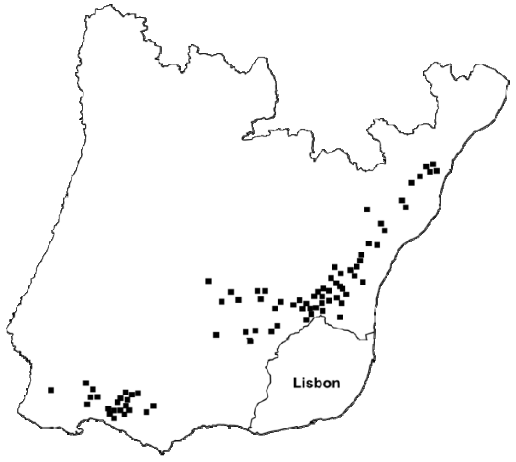
“Casal de Cambra” is an example of the kind of self-organized processes that supported the evolution of NMAL. Although single-family houses were predominant (at least in the first stage of formation) [
24] and their construction was mainly conducted by their owners, the scale of the settlement—originally a large parcel—can be understood as a large urbanization project (concerning only its total area). The spatial distribution of other informal settlements throughout NMAL (identified in a 1977 study [
24]) seems to bear some relation between form and process and the aforementioned
non-sequential transitions (
Figure 10).
Figure 10.
Informal settlements in NMAL, outside Lisbon city, by 1971 (after [
24]).
Figure 10.
Informal settlements in NMAL, outside Lisbon city, by 1971 (after [
24]).
The difference for pre-determined non-sequential transitions will probably lie in the time scale of both kinds of non-sequential transitions. For lack of intermediate time periods it is not possible to ascertain this hypothesis at present.
5. Discussion and Conclusions
We explored the relation between local fractal dimension and the development of the built-up areas of NMAL, for the period between 1960 and 2004. Based on the GLSE function it was possible to break-up NMAL into the five types of regions that GLSE defines.
The spatio-temporal analysis performed here shows the presence of two co-evolving growth-processes: fragmentation/dispersion and consolidation/compactification. These processes can be identified resorting to the following core growth types of built-up area changes over time: growth-type 1) new areas that emerge isolated; growth-type 2) existing areas that grow contiguously, and growth-type 3) existing areas that grew and aggregated with one or more neighboring areas. Based on these three core growth-types it was possible to identify cases where sprawl areas have changed into more compact and contiguous ones, thus recognizing sprawl as a process in the evolution of territories.
In NMAL, we found that the fragmentation and consolidation processes co-evolved during the first time period (1960–1990), whereas in the second time period (1990–2004) the consolidation process dominated, as a result of the overall compactification of NMAL. Given the lack of an efficient planning system in Portugal, the data available does not enable us to ascertain whether planning is able to control the sizeable fragmentation process observed in NMAL. Clearly, further assessment is needed, possibly in connection with other urban areas where planning is known to be well-established.
The analysis performed on the evolution of the five region types revealed different types of transitions among region types: (i) sequential (forward) transitions, (ii) reverse transitions and iii) non-sequential (forward) transitions.
Sequential transitions should be linked to more self-organized processes with smooth growth. Reverse transitions occur when the increase in built-up area contributes to a more disperse pattern and should thus be rapidly identified in areas where sprawl must be controlled. They can also contribute to the intensification of a fragmentation process if not supported by strategic planning actions.
In theory, non-sequential (forward) transitions should be identified with top-down planned interventions (as major real estate investment projects) which can be used by planning agencies as a means to rapidly enforce a consolidation process. However, we have also shown how non-sequential transitions may result from self-organized processes as in the emergence of informal settlements.
The spatial distribution of each of the aforementioned types of transitions suggests a probable link between their form and function in the context of the metropolitan area: for example, non-sequential transitions usually emerge near a pre-existing main nucleus (e.g., Lisbon city and main suburbs), whereas sequential transitions (especially those from more dispersed types) tend to spread throughout the territory.
Region type 3 played a pivotal role in both fragmentation and consolidation processes, and thus likely connects both processes. The number of possible configurations given by GLSE and its rate of change are higher for this type than for any of the other types. Hence, planning agencies should take special attention on the location and evolution of cells of and into this type. More specifically, planning agencies should consider two main options, depending on their medium/long term strategy for the development of the territories under their regulation:
If the intention is to promote sprawl, then they should promote the emergence of new Type 3 areas but control growth of existing Type 3 areas into Types 4 and 5. If the intention is to promote compact areas, then they should control the emergence of new Type 3 areas but promote growth of existing Type 3 areas into Types 4 and 5.
Compact or fragmented spatial systems should thus be achieved by the interplay between pre-existing and new Type 3 areas and their spatial context regarding more compact areas, such as Types 4 and 5.
Although GLSE can help to quickly identify areas that should be intervened it cannot distinguish or characterize (in terms of internal quality and functioning) two cells of the same type. Consequently, even if it is possible to use this model to assess for example whether more compact areas should be promoted and where—at the metropolitan or municipality scales—it will not be possible to ascertain their quality regarding urban design, functions and behavior—at the cell scale.

 ,
, 


