Entropy Evaluation Based on Value Validity

Abstract

Besides its importance in statistical physics and information theory, the Boltzmann-Shannon entropy S has become one of the most widely used and misused summary measures of various attributes (characteristics) in diverse fields of study. It has also been the subject of extensive and perhaps excessive generalizations. This paper introduces the concept and criteria for value validity as a means of determining if an entropy takes on values that reasonably reflect the attribute being measured and that permit different types of comparisons to be made for different probability distributions. While neither S nor its relative entropy equivalent S* meet the value-validity conditions, certain power functions of S and S* do to a considerable extent. No parametric generalization offers any advantage over S in this regard. A measure based on Euclidean distances between probability distributions is introduced as a potential entropy that does comply fully with the value-validity requirements and its statistical inference procedure is discussed.

1. Introduction

Consider that p₁,..., p_n, with ${\displaystyle \sum _{i=1}^n}{p}_i=1$, are the probabilities of a set of n quantum states accessible to a system or of a set of n mutually exclusive and exhaustive events of some statistical experiment. Thus, p_i is the probability of the system being in state i or of event i occurring ( i = 1,..., n ). The entropy (of the system or set of events) is then defined as:

$$S=-k\sum _{i=1}^n{p}_i\hspace{0.17em}\text{log\hspace{0.17em}}{p}_i$$

(1)

where k is some positive constant and where the logarithm is the natural one. In statistical mechanics, k may be Boltzmann’s constant, while, in information theory, k = 1/log2 so that $S=-{\displaystyle \sum _{i=1}^n}{p}_i\hspace{0.17em}{\text{log}}_2\hspace{0.17em}{p}_i$ and the unit of measurement becomes bits as introduced by Shannon [1]. When deriving Equation (1) axiomatically from some basic required properties (axioms), k becomes an arbitrary constant (e.g., [2,3]). For convenience, we shall set k = 1 throughout this paper.

The entropy S, which provides a link between statistical mechanics and information theory, is interpreted somewhat differently in the two fields. In statistical mechanics, entropy is often considered to be a measure of the disorder of a system, although it may be argued that a more appropriate measure of disorder is the following dimensionless relative entropy [3] (pp. 366–357):

$$S^{*}=\frac{S}{\text{log\hspace{0.17em}}n}=-\sum _{i=1}^n{p}_i\hspace{0.17em}{\text{log}}_n\hspace{0.17em}{p}_i\in [0,1]$$

(2)

In information theory, S is typically interpreted as a measure of the uncertainty, information content, or randomness of a set of events, while S^* in (2) is considered as a measure of efficiency of a noise-free communication channel and 1− S^* as a measure of its redundancy [4] (pp. 109–110).

Boltzmann [5] had used the function S in Equation (1) (or its continuous analog), but what Shannon [1] “did was to give a universal meaning to the function −∑p_i log p_i and thereby make it possible to find other applications [6] (p. 476)”. This function has indeed proved to be remarkably versatile and used as a measure of a variety of attributes in various fields of study, ranging from ecology (e.g., [7]) to psychology (e.g., [8]). It has also resulted in literally infinitely many alternative entropy formulations and generalizations such as the parameterized families of entropies given in

Table 1. Parameterized families of entropies.

Formulation	Parameter Restrictions	Source
$S_1=\frac{1}{1-\alpha }\text{log}{\displaystyle \sum _{i=1}^n}{p}_i^{\alpha }$	α > 0	Rényi [10,11]
$S_2=\frac{1}{2^{1-\alpha }-1}\left({\displaystyle \sum _{i=1}^n}{p}_i^{\alpha }-1\right)$	α > 0	Havrda and Charvát [12]
$S_3=\frac{k}{1-\alpha }\left({\displaystyle \sum _{i=1}^n}{p}_i^{\alpha }-1\right)$	−∞ < α < ∞, k constant	Tsallis [13]
$S_4=\frac{1}{\delta -\alpha }\text{log\hspace{0.17em}}\left(\frac{{\displaystyle \sum _{i=1}^n}{p}_i^{\alpha }}{{\displaystyle \sum _{i=1}^n}{p}_i^{\delta }}\right)$	α, δ > 0	Kapur [14], Aczél and Daróczy [15]
$S_5=\frac{\alpha }{1-\alpha }\left[{\left({\displaystyle \sum _{i=1}^n}{p}_i^{\alpha }\right)}^{1/\alpha }-1\right]$	α > 0	Arimoto [16]
$S_6=\frac{1}{2^{1-\beta }-1}\left[{\left({\displaystyle \sum _{i=1}^n}{p}_i^{\alpha }\right)}^{(\beta -1)/(\alpha -1)}-1\right]$	α, β > 0	Sharma and Mittal [17]
$S_7=\frac{1}{2^{1-\alpha }-1}\left[\frac{{\displaystyle \sum _{i=1}^n}{p}_i^{\alpha +\delta -1}}{{\displaystyle \sum _{i=1}^n}{p}_i^{\delta }}-1\right]$	α > 0, α + δ −1 > 0	Rathie [18]
$S_8=\lambda \left[{\left(\frac{{\displaystyle \sum _{i=1}^n}{p}_i^{\alpha }}{{\displaystyle \sum _{i=1}^n}{p}_i^{\delta }}\right)}^{\beta }-1\right]$	0 < α < 1 ≤ δ, βλ > 0; or, 0 ≤ δ ≤ 1 < α, βλ < 0	Kvålseth [19–21]
$S_9=\frac{\alpha }{2^{\beta }-1}(2^{\beta S_i}-1)$	α, β > 0	Morales et al. [22]
$S_{10}={\displaystyle \sum _{i=1}^n}{p}_i^{\alpha }{(-\text{log\hspace{0.17em}}{p}_i)}^{\beta }$	α, β positive integers	Good [23]
$S_{11}=-\frac{1}{{\displaystyle \sum _{i=1}^n}{p}_i^{\alpha }}{\displaystyle \sum _{i=1}^n}{p}_i^{\alpha }\hspace{0.17em}\text{log\hspace{0.17em}}{p}_i$		Aczél and Daróczy [15]

Notes: The Greek letters used for the parameters differ from some of those used by the authors. When indeterminate forms 0/0 occur from certain parameter values (e.g, α = 1 for S₁ or β = 1 for S₆ ), the entropies are defined in their limits (e.g., as α → 1 or β → 1) using L’Hôpital’s rule.

and for each of which the S in Equation (1) is a particular member. The real utility or contributions of those generalization efforts may be questioned, with some calling them “mindless curve-fitting” and stating that “The ratio of papers to ideas has gone to infinity” [9].

This paper is concerned with the use and misuse of S and S^* in Equations (1) and (2) and other proposed entropies. Whatever an entropy measure is being used for, it is not uncommon for comparisons to be made between differences in entropy values and for statements or implications to occur about the absolute and relative values of the attributes (characteristics) being measured by means of the entropy. This can lead to incorrect and misleading results and conclusions unless certain conditions are met as discussed in this paper. If, using a simplified notation, e₁, e₂,... denote the values of a generic entropy E for the probability distributions P_n = (p₁,... p_n ), Q_m = (q₁,..., q_m ),..., the various types of potential comparisons may be defined as follows:

$$Size\hspace{0.17em}(order)\hspace{0.17em}comparison:e_1>e_2$$

(3a)

$$Difference\hspace{0.17em}comparison:e_1-e_2>e_3-e_4$$

(3b)

$$Proportional\hspace{0.17em}difference\hspace{0.17em}comparison:e_1-e_2>c(e_3-e_4)$$

(3c)

where c is a constant.

In particular, we shall address the following fundamental questions: Which conditions on an entropy are required for the comparisons in Equation (3) to be valid or permissible? Does S or S^* in Equations (1) and (2) meet such valid comparison conditions, and if not, are there functions of S or S^* that do? Do any of the entropy families in Table 1 have members that are superior to S in this regard? If none of those entropies meet such conditions, is there an alternative entropy formulation that does?

2 Entropy Properties

2.1. Properties of S

Although the properties of S(P_n ), or simply S, in Equation (1) are discussed in various textbooks (e.g., [2–4,10,24]), they will be briefly outlined here so that we can conveniently refer to them throughout this paper. Some of the most important ones are as follows:

(P1)

S is a continuous function of all its arguments p₁,..., p_n (so that small changes in some of the p_i ’s result in only a small change in the value of S).

(P2)

S is (permutation) symmetric in the p_i (i = 1,..., n).

(P3)

S is zero-indifferent (expansible), i.e., the addition of some state(s) or event(s) with zero probability does not change the value of S, or formally:

$$S(p_1,\dots ,p_n,0,\dots ,0)=S(p_1,\dots ,p_n)$$

(P4)

S attains its extremal values for the two probability distributions:

$$P_n^0=(1,\hspace{0.17em}0,\dots ,\hspace{0.17em}0),\hspace{0.17em}{P}_n^1=\left(\frac{1}{n},\dots ,\frac{1}{n}\right)$$

(4)

so that, for any distribution P_n = (p₁,..., p_n ):

$$S\left(P_n^0\right)\le S(P_n)\le S(P_n^1)$$

(P5)

$S(P_n^1)$ is strictly increasing in n for $P_n^1$ in Equation (4).

(P6)

S is strictly Schur-concave and hence, if P_n is majorized by Q_n (denoted by ≺):

$$P_n\prec Q_n\Rightarrow S(P_n)\ge S(Q_n)$$

with strict inequality unless Q_n is simply a permutation of P_n.

(P7)

S is additive in the following sense. If {p_ij} in the joint probability distribution for the quantum states for two parts of a system or for the events of two statistical experiments, with marginal probability distributions {p_i+} and {p_{+ j}} where $p_{i+}={\displaystyle \sum _{j=1}^m}{p}_{ij}$ and $p_{+j}={\displaystyle \sum _{i=1}^n}{p}_{ij}$ for i = 1,..., n and j = 1,..., m, then, under independence:

$$S(\{p_{ij}\})=S(\{p_{i+}{p}_{+j}\})=S(\{p_{i+}\})+S(\{p_{+j}\})$$

(5)

Most of these properties would seem to be necessary and desirable for any entropy. One could argue about the absolute necessity of Property P7 (e.g., [25]) and among the families of entropies in Table 1, only S₁ and S₄ have this property. The essential Property P6 is a precise way of stating that the value of S increases as components of a probability distribution become “more nearly equal”, i.e., S(P_n ) > S(Q_n ) if the components of P_n are “more nearly equal” or ”less spread out” than those of Q_n. In terms of majorization, and by definition [26], if the components of P_n are ordered such that:

$$p_1\ge p_2\ge \dots \ge p_n$$

(6)

and similarly for Q_n, then:

$$P_n\prec Q_n\hspace{0.17em}\text{if\hspace{0.17em}}\sum _{i=1}^j{p}_i\le \sum _{i=1}^j{q}_i,j=1,\dots ,n-1$$

(7)

with ${\displaystyle \sum _{i=1}^n}{p}_i={\displaystyle \sum _{i=1}^n}{q}_i=1$. Of course, not all P_n and Q_n are comparable with respect to majorization.

2.2. Valid Comparison Conditions

If an entropy has the above Properties P1–P6, there would seem to be no particular reason to doubt that size (order) comparisons are reasonable or permissible. Thus, for S and Equation (1) with k = 1 and for, say, $P_3^{(1)}=(0.90,0.05,0.05)$ and $P_2^{(2)}=(0.70,\hspace{0.17em}0.30)$ so that $S(P_3^{(1)})=0.39$ and $S(P_2^{(2)})=0.61$, it would be reasonable to conclude that the disorder or uncertainty is greater in the second case than in the first. However, for the additional probability distributions $P_2^{(3)}=(0.8,0.2)$ and $P_4^{(4)}=(0.70,0.15,0.10,0.05)$, the result $S(P_2^{(2)})-S(P_3^{(1)})=0.22$ and $S(P_4^{(4)})-S(P_2^{(3)})=0.41$ simply states that the difference in S-values of 0.22 is less than that of 0.41. There is, however, no basis for assuming or suggesting that this result necessarily reflects the true differences in the disorder of the four systems or the uncertainty of the four sets of events. For such comparisons to be valid, additional conditions need to be imposed. We shall determine such validity conditions in a couple of different ways.

In measurement theory, “Validity describes how well the measured variable represents the attribute being measured, or how well it captures the concept which is the target of measurement” [27] (p. 129). While there are different forms of validity, we shall use value validity and define it as follows:

Definition: A measure has value validity if all its potential values provide numerical representations of the size (extent) of the attribute being measured that are true or realistic with respect to some acceptable criterion.

To determine the conditions for an entropy to have value validity, we shall use the recently introduced lambda distribution defined as:

$$P_n^{\lambda }=\left(1-\lambda +\frac{\lambda }{n},\frac{\lambda }{n},\dots ,\frac{\lambda }{n}\right),\lambda \in [0,1]$$

(8)

where λ is a parameter that reflects the uniformity or evenness of the distribution [28]. The $P_n^0$ and $P_n^1$ in Equation (4) are particular (extreme) cases of this distribution. In fact, $P_n^{\lambda }$ is a weighted mean of $P_n^0$ and $P_n^1$, i.e.,:

$$P_n^{\lambda }=\lambda P_n^1+(1-\lambda )P_n^0$$

(9)

For a generic entropy E that is (strictly) Schur-concave (Property P6), and from the majorization $P_n^1\prec P_n\prec P_n^0$ for any given P_n as is easily verified from Equations (6) and (7), it follows that:

$$E(P_n)=E(P_n^{\lambda })\hspace{0.17em}\text{for\hspace{0.17em}a\hspace{0.17em}unique\hspace{0.17em}}\lambda$$

(10)

Consequently, validity conditions on E(P_n ) can equivalently be formulated in terms of $E(P_n^{\lambda })$.

By considering $P_n^{\lambda },P_n^0$, and $P_n^1$ as points (vectors) in n-dimensional space, Euclidean distances are then the logical choice as the basis of a criterion for the value validity of entropy E. Then, the following ratio equality presents itself as the natural and obvious requirement:

$$\frac{E(P_n^1)-E(P_n^{\lambda })}{E(P_n^1)-E(P_n^0)}:=\frac{d(P_n^{\lambda },P_n^1)}{d(P_n^0,P_n^1)}=1-\lambda$$

(11)

Besides the standard Euclidean distance function d used in Equation (11), the same result 1 − λ would be obtained for all members of the Minkowski class of distance metrics. With $E(P_n^0)=0$ since there is no disorder or uncertainty when one p_i = 1 (and the other p_i ’s equal 0) or when n = 1, (11) can be expressed as:

$$E(P_n^{\lambda })=\lambda E(P_n^1)$$

(12)

and, in terms of the relative entropy:

$$E^{*}(P_n^{\lambda })=\frac{E(P_n^{\lambda })}{E(P_n^{\text{1}})}=\lambda$$

(13)

for all n and λ. This formulation is also an immediate consequence of (9), i.e.:

$$E(P_n^{\lambda })=E[\lambda P_n^1+(1-\lambda )P_n^0]=\lambda E(P_n^1)+(1-\lambda )E(P_n^0)=\lambda E(P_n^1)\hspace{0.17em}\text{for\hspace{0.17em}}E(P_n^0)=0$$

(14)

If we accept $E(P_n^1)=\text{log\hspace{0.17em}}n$ as a reasonable maximum entropy for any given n, which is that of S in Equation (1) (with k = 1), then Equation (12) would become:

$$E(P_n^{\lambda })=\lambda \hspace{0.17em}\text{log\hspace{0.17em}}n$$

(15)

However, a reasonable and justifiable alternative would clearly be $E(P_n^1)=n-1$ so that Equation (12) becomes:

$$E(P_n^{\lambda })=(n-1)\lambda$$

(16)

Of course, both expressions in Equations (15) and (16) give $E(P_n^{\lambda })=0$ for n = 1 as is only reasonable.

The $E(P_n^1)=n-1$ and Equation (12) also follow from simple functional equations. With $E(P_n^1)=f(n)$, it seems reasonable and most intuitive to suggest that increasing n by an integer value m (m < n) should result in the same absolute change in the value of the function f as when n is reduced by the same amount m, i.e.,:

$$f(n+m)-f(n)=f(n)-f(n-m)$$

(17)

The general solution to this functional equation is:

$$f(n)=a+bn$$

(18)

where a and b are arbitrary real constants [29] (p. 82). Also, Equation (18) is the solution of Jensen’s functional equation for integers ([29] (p. 43), i.e.,:

$$f\left(\frac{n+m}{2}\right)=\frac{f(n)+f(m)}{2}$$

(19)

Since f(1)=0, Equation (18) becomes f (n) = b(n − 1) and hence $E(P_n^1)=n-1$ for b = 1.

If, instead of Equation (17), one proposes:

$$f(nm)=f(n)+f(m)$$

(20)

then the most general solution would be f (n) = a logn with arbitrary constant a [29] (p. 39). By setting a = 1 and hence $E(P_n^1)=\text{log\hspace{0.17em}}n$, then, instead of Equation (16), Equation (12) becomes Equation (15).

Similarly, for any given (fixed) n, $E(P_n^{\lambda })$ becomes a function g of λ only and for which it is proposed that:

$$g(\lambda +\mu )-g(\lambda )=g(\lambda )-g(\lambda -\mu )$$

(21)

where μ is such that 0 ≤ λ + μ ≤ 1 and 0 ≤ λ − μ ≤ 1, with the general solution of Equation (21) being:

$$g(\lambda )=c+d\lambda$$

(22)

with arbitrary constants c and d [29] (p.82). Since $E(P_n^0)=g(0)=0$ and $E(P_n^1)=g(1)=d$, Equation (22) results in Equation (12).

Consequently, different lines of reasoning lead to Equations (12) and (15) or Equation (16) as conditions for an entropy E to have value validity and therefore making the difference comparisons in Equations (3b) and (3c) permissible. The basis for those conditions are the distance criterion in Equation (11), the mean-value relationship in Equation (14), and the difference relationships represented by the functional equations in Equations (17), (19)–(21). Those functional equations also directly support the validity of the comparisons in Equations (3b) and (3c).

3. Value-Valid Functions of S and S^*

It is immediately apparent that neither S in Equation (1) nor S^* in Equation (2) meet those validity conditions. It is found that S and S^* consistently overstate the true extent of the attribute being measured, i.e., the attribute of system disorder or event uncertainty. Consider, for example, the lambda distribution in Equation (8) with λ = 0.5 and n = 4, i.e., $P_4^{0.5}=(0.625,0.125,0.125,0.125)$ for which S = 1.07 and S^* = 0.77, which are, respectively, substantially greater than the values (0.5) log 4 = 0.69 and 0.5 as required by Equations (15) and (13). Each element of the distribution $P_4^{0.5}$ has the same distance from each element of $P_n^1=(0.25,0.25,0.25,0.25)$ as it does from each element of $P_n^0=(1,0,0,0)$, i.e., $P_4^{0.5}$ is the midpoint between $P_4^0$ and $P_4^1$. Clearly, the midrange (0 + log4)/2 = 0.69 would be the only reasonable entropy value and the midrange (0+1)/2 = 0.5 the only reasonable relative entropy value, which are consistent with Equations (15) and (13). Also, one distribution P₄ for which $S(P_4)=S(P_4^{0.5})$ as in Equation (10) is found by trial and error to be P₄ = (0.6, 0.2, 0.14, 0.06).

As another simple example, consider P₃ = (0.8, 0.15, 0.05) for which S = 0.61 and S^* = 0.56. Since this P₃ -distribution is much closer to $P_3^0=(1,\hspace{0.17em}0,\hspace{0.17em}0)$ than it is to $P_3^1=(1/3,1/3,1/3)$ and since S ∈ [0, 1.10] for n = 3 and since S^* ∈ [0, 1], these values of S = 0.61 and S^* = 0.56 are unreasonably large. By comparison, for $S(0.8,0.15,0.5)=\text{S}({\text{P}}_3^{\lambda })$ in Equation (10), it is found that λ = 0.282 so that, from Equations (13) and (15), 0.282log3 = 0.31 and 0.28, respectively, would have been appropriate values, rather than 0.61 and 0.56, had the entropy (with upper bound log n) had value validity. When comparing the results from these two examples with the respective S-values of 1.07 and 0.61, it would not be a valid inference that the disorder (uncertainty) in the first case was about 75% greater than in the second case (i.e., as a particular case of Equation (3c)). This result would only apply to the S-values themselves and not to the attribute that S is supposed to measure (i.e., the disorder or uncertainty). The appropriate and valid comparison should be between the above entropy values of 0.69 and 0.31, showing a 123% increase in disorder (uncertainty). Even though S and S^* do not meet the conditions for valid difference comparisons, perhaps some functions of S and S^* do. We shall address this next.

3.1. The Case of S

In order to satisfy the validity requirement in Equation (15), we shall explore if there exists a function (or transformation) f such that:

$$S(P_n^{\lambda })=f(\lambda \hspace{0.17em}\text{log\hspace{0.17em}}n)$$

(23)

from which a transformed entropy S_T could be obtained as:

$$S_T(P_n^{\lambda })=\lambda \hspace{0.17em}\text{log\hspace{0.17em}}n=f^{-1}[S(P_n^{\lambda })]=g[S(P_n^{\lambda })]$$

(24)

where $P_n^{\lambda }$ is again the distribution defined in Equation (8). From the graphs of $S(P_n^{\lambda })$

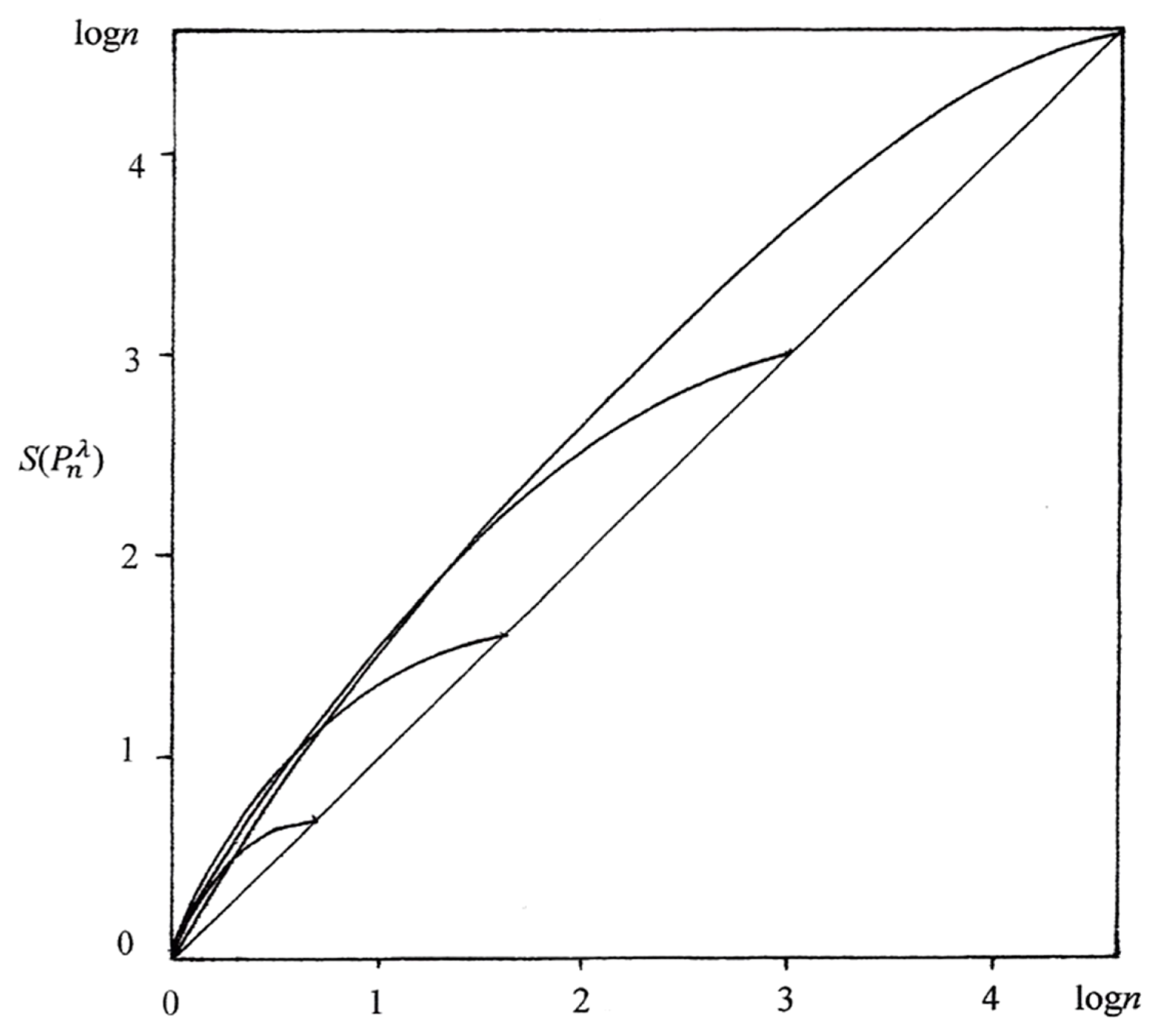
versus λ logn for some different values of n as shown in Figure 1, it is clear that no such function f exists for all λ and n. It is also evident from Figure 1 that S overstates the degree of disorder (uncertainty) throughout the range from 0 to log n and for different n. The absolute extent of such overstatement or lack of value validity appears to be greatest when S roughly equals (4/3) log n.

Nevertheless, it would appear from Figure 1 that at least a reasonable degree of approximation could be achieved from Equations (23) and (24) if we restrict those functions to cases when, say, S ≤ 0.8logn, or S* ≤ 0.8 for all n. When the function (model) S = α (λ logn)^β is fitted to the different values of n and λ in

Table 2. Values of S in Equation (1) (with k = 1), S^* in Equation (2)S_T in Equations (25)–(26) and $S_T^{*}$ in Equation (28) for the lambda distribution $P_n^{\mathrm{\lambda }}$ in Equation (8) with varying n and λ.

n	λ	λ and n	S	S*	ST	$S_T^{*}$
2	0.1	0.07	0.20	0.29	0.08	0.10
2	0.3	0.21	0.42	0.61	0.20	0.31
2	0.5	0.35	0.56	0.81	-	0.51
2	0.7	0.49	0.65	0.94	-	0.72
2	0.9	0.62	0.69	0.99	-	0.88
5	0.1	0.16	0.39	0.24	0.19	0.09
5	0.3	0.48	0.88	0.55	0.51	0.29
5	0.5	0.80	1.23	0.76	0.78	0.50
5	0.7	1.13	1.46	0.91	-	0.71
5	0.9	1.45	1.59	0.99	-	0.92
10	0.1	0.23	0.50	0.22	0.25	0.09
10	0.3	0.69	1.18	0.51	0.74	0.28
10	0.5	1.15	1.68	0.73	1.15	0.50
10	0.7	1.61	2.04	0.89	-	0.71
10	0.9	2.07	2.27	0.98	-	0.90
20	0.1	0.30	0.59	0.20	0.31	0.08
20	0.3	0.90	1.44	0.48	0.95	0.28
20	0.5	1.50	2.09	0.70	1.51	0.49
20	0.7	2.10	2.60	0.87	-	0.71
20	0.9	2.70	2.93	0.98	-	0.92
50	0.1	0.39	0.70	0.18	0.39	0.08
50	0.3	1.17	1.75	0.45	1.21	0.28
50	0.5	1.96	2.60	0.66	1.99	0.48
50	0.7	2.74	3.29	0.84	-	0.70
50	0.9	3.52	3.80	0.97	-	0.92
100	0.1	0.46	0.78	0.17	0.44	0.08
100	0.3	1.38	1.97	0.43	1.41	0.28
100	0.5	2.30	2.97	0.64	2.35	0.49
100	0.7	3.22	3.80	0.83	-	0.72
100	0.9	4.14	4.44	0.96	-	0.91

for S* ≤ 0.8, regression analysis results in the parameter estimates α̂ = 1.52 and β̂ = 0.78. When these estimates are replaced with the nearest fraction (for convenience) 3/2 and 4/5 and when this fitted function is then inverted as in Equation (24), we obtain the transformed entropy:

$$S_T(P_n^{\lambda })={\left[\left(\frac{2}{3}\right)S(P_n^{\lambda })\right]}^{5/4}\hspace{0.17em}\text{for\hspace{0.17em}}{S}^{*}(P_n^{\lambda })\le 0.8$$

(25)

so that, for any probability distribution P_n = (p₁,..., p_n ) and from Equation (10):

$$S_T(P_n)={\left[\left(\frac{2}{3}\right)S(P_n)\right]}^{5/4}\hspace{0.17em}\text{for\hspace{0.17em}}{S}^{*}(P_n)\le 0.8$$

(26)

The values of $S_T(P_n^{\lambda })$ in Equation (25) for various λ and n as given in Table 2 are quite comparable with the corresponding values of λ log n. In fact, the coefficient of determination, when properly computed [30], is found to be $R^2=1-\mathrm{\Sigma }{[\lambda \hspace{0.17em}\text{log\hspace{0.17em}}n-S_T(P_n^{\lambda })]}^2/\mathrm{\Sigma }{(\lambda \hspace{0.17em}\text{log\hspace{0.17em}}n-\overline{\lambda \hspace{0.17em}\text{log\hspace{0.17em}}n})}^2=0.998$, showing that about 99% of the variation of λ log n is explained (accounted for) by the model in Equation (25).

The entropy S_T has all of the same Properties P1–P6 as does S, but it does not have the additivity Property P7. Of course, S_T has the limitation that it is defined for the restricted range from 0 to [(2/3)(.8 log n)]^5/4. However, S_T in Equation (26) does approximately meet the requirement in Equation (15) for its limited range so that difference comparisons as in Equations (3b) and (3c) are reasonably valid.

3.2. The Case of S^*

For the relative entropy S^* ∈[0,1] in Equation (2), and in order to meet the validity condition in Equation (12) with $E(P_n^1)=1$, a function f is needed such that $S^{*}(P_n^{\lambda })=f(\lambda ,n)$ and from which a transformed relative entropy $S_T^{*}\in [0,\hspace{0.17em}1]$ follows as:

$$S_T^{*}(P_n^{\mathrm{\lambda }})=\mathrm{\lambda }=g[S^{*}(P_n^{\mathrm{\lambda }}),\hspace{0.17em}n]$$

(27)

It is apparent from Figure 1 that the functions f and g have to have the integer n as a variable. By exploring alternative functions or models for different n and λ, using regression analysis, and expressing parameter estimates as convenient fractions, the following result is obtained:

$$S_T^{*}=1-{[1-{(S^{*})}^{4/3}]}^{\mathrm{\alpha }},\hspace{0.17em}\mathrm{\alpha }=(1/2){(n-1)}^{1/9}$$

(28)

where S^* stands for either $S^{*}(P_n^{\mathrm{\lambda }})$ or S^* (P_n) and the corresponding $S_T^{*}$ stands for either $S_T^{*}(P_n^{\mathrm{\lambda }})$ or $S_T^{*}(P_n)$.

This function (model) in Equation (28) does indeed provide excellent fit to different data points (n, λ) as seen from the results in Table 2. The values of $S_T^{*}(P_n^{\lambda })$ are nearly equal to the values of λ for different n. The small residuals $\lambda -S_T^{*}$ in Table 2 have no clear pattern that would indicate any particular inadequacy with Equation (28). The coefficient of determination, when properly computed [30], is found from Table 2 to be $R^2=1-\mathrm{\Sigma }{(\lambda -S_T^{*})}^2/\mathrm{\Sigma }{(\lambda -\overline{\lambda })}^2=0.997$, indicating that nearly all of the variation in the chosen λ-values is explained by Equation (28).

While the S_T in Equations (25) and (26) is only defined for S^* ≤ 0.8, the $S_T^{*}$ in Equation (28) is appropriate for all $S_T^{*}$ and S^*. Being a strictly increasing function of S^* = S/log n for any given n, $S_T^{*}$ has some of the same properties as S given in Section 2.1 with some obvious exceptions. However, $S_T^{*}$ has the important advantage over S* of satisfying, to a high degree of approximation, the condition in Equation (12) with $S_T^{*}(P_n^1)=1$, making difference comparisons as in Equations (3b) and (3c) reasonably valid for $S_T^{*}$. Of course, neither $S_T^{*}$ nor S^* are zero-indifferent (Property P3) unless n is replaced by n⁺ where n⁺ is the number of positive elements of P_n = (p₁,…p_n), or formally stated:

$$n^{+}=\#\{1\le i\le n:p_i>0\}$$

(29)

It may also be noted that log₂ n⁺ is frequently referred to as Hartley’s measure or entropy ([24], Chapter 2) after Hartley [31].

For the interesting binary case; Equation (28) simplifies to:

$$S_T^{*}=1-\sqrt{1-{(S^{*})}^{4/3}}\hspace{0.17em}\text{for\hspace{0.17em}}n=2$$

(30)

and noting that:

$$S^{*}(P_2)=-\sum _{i=1}^2{p}_i\hspace{0.17em}\text{log}{p}_i/\text{log}2=-\sum _{i=1}^2{p}_i\hspace{0.17em}{\text{log}}_2\hspace{0.17em}{p}_i$$

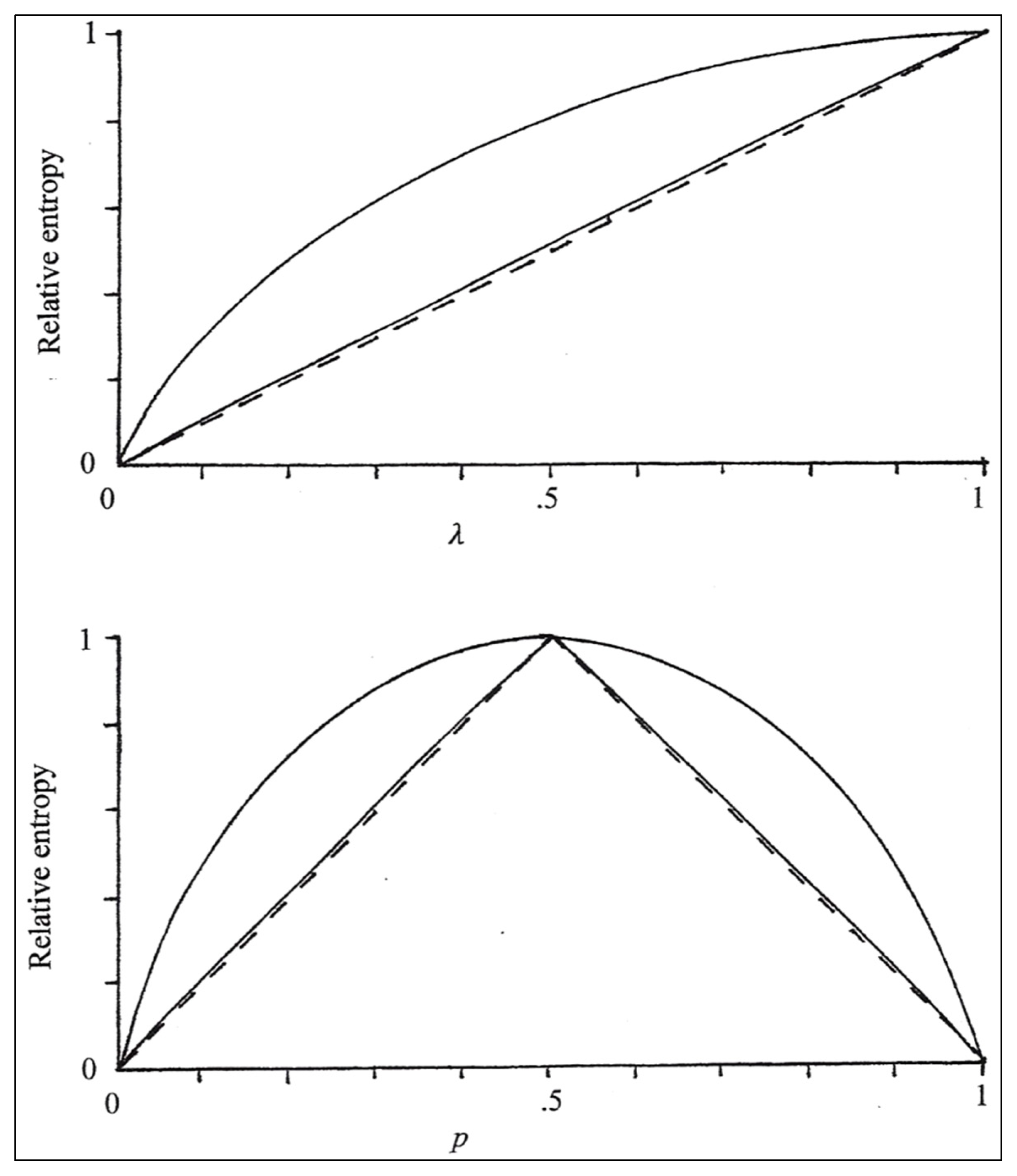
Figure 2 shows a comparison between $S_T^{*}$ and S^* for distribution $P_2^{\lambda }=(1-\lambda /2,\lambda /2)$ (upper graph) and for P₂ = (1 − p,p) (lower graph), with the latter form of the distribution typically being used for depicting binary entropies (e.g., [4,24]). The dashed lines represent the entropy requirement for value validity in Equation (13), which, for the upper and lower graphs becomes, respectively:

$$E^{*}(P_2^{\lambda })=\lambda ,\hspace{0.17em}{E}^{*}(1-p,p)=1-\mid 1-2p\mid$$

(31)

Note that, while the derivative of E^*(1 − p, p) with respect to p in Equation (31) does not exist at p = 0.5, E^* (1−p, p) is continuous at p = 0.5 (Property P1).

It may perhaps be tempting to use $S_T^{*}$ in Equation (28) to propose the following entropies:

$$S_T^{\prime }=(\text{log\hspace{0.17em}}n)S_T^{*},\hspace{0.17em}{S}_T^{″}=(n-1)S_T^{*}$$

(32)

which would, respectively, comply with Equations (15) and (16), at least to a high degree of approximation. If, instead of n, the n⁺ in Equation (29) is used in Equation (32) and for $S_T^{*}$ in Equation (28), then those two potential entropies $S_T^{\prime }$ and $S_T^{″}$ would also be zero-indifferent (Property P3). However, neither $S_T^{\prime }$ nor $S_T^{″}$ can be acceptable entropies as exemplified by the two distributions P₄ = (0.40, 0.35, 0.24, 0.01) and Q₄ = (0.40, 0.35, 0.24, 0) for which S(P₄) = 1.12 and S(Q₄) = 1.08 whereas, from Equations (32) and (28) using n⁺, $S_T^{\prime }(P_4)=0.76,\hspace{0.17em}{S}_T^{\prime }(Q_4)=0.94,\hspace{0.17em}{S}_T^{″}(P_4)=1.50$ and $S_T^{″}(Q_4)=1.72$. That is, in spite of the majorization P₄ ≻ Q₄ when any reasonable entropy should be greater for P₄ than for Q₄ (Property P6), both $S_T^{\prime }$ and $S_T^{″}$ give the opposite result. It is easy to find other examples with the same results.

4. Assessment of Entropy Families

For a parameterized family of entropies S_i, such as those defined in Table 1, to be viable beyond being an interesting mathematical exercise or a generalization for its own sake, one could certainly argue that S_i would need to meet some conditions lacking by S in Equation (1). First, S_i should have some properties that may be considered important or desirable and that S is lacking. Second, the flexibility provided by the incorporation of one or more parameters into the formulation of S_i should be justifiable by the parameter(s) having some meaning or interpretation relative to the characteristic (attribute) that S_i is supposed to measure.

With respect to the first condition, it is rather obvious from the expressions in Table 1 that none of those entropy families would be favored over S in Equation (1) in terms of their properties. In fact, some of those entropies are even lacking the essential Schur-concavity property (Property P6 in Section 2.1). The entropy S₃ in Table 1, which is a particular subset of S₈ with β = δ = 1 and λ = k/(1 − α), and which was defined for all real α, is strictly Schur-concave only for α ≥ 0. This follows immediately from the fact that, with the p_i′s ordered as in Equation (6), the partial derivative $\partial S_3/\partial p_i=k[\alpha /(1-\alpha )]p_i^{\alpha -1}$ is increasing in i = 1,…, n only if α > 0 and strictly so if the inequalities in Equation (6) are all strict [26] (p.84). For the limiting case when α → 0, S₃ reduces to (1), which is strictly Schur-concave [26] (p. 101). Similarly, S₁₀ was defined by Good [23] for non-negative integer values of α and β, but is not Schur-concave for all such α and β values. Baczkowski et al. [32] extended S₁₀ to permit α and β to take on real values and determined the rather restrictive (α, β) regions for the Schur-concavity of S₁₀.

A brief comment is warranted about the potential case when the probability distribution p_n = (p₁,…,p_n) is possibly incomplete, i.e., when ${\displaystyle \sum _{i=1}^n}{p}_i\le 1$ [10,11]. Then, setting λ = k/(1 − α) for some constant k and β = δ = 1, the S₈ in Table 1 becomes:

$$S_{8\mathrm{\alpha }}=\frac{k}{1-\mathrm{\alpha }}\left(\frac{{\displaystyle \sum _{i=1}^n}{p}_i^{\mathrm{\alpha }}}{{\displaystyle \sum _{i=1}^n}{p}_i}-1\right),\hspace{0.17em}\mathrm{\alpha }>0$$

(33)

In the limiting case when α α 1, and using L’Hôpital’s rule, Equation (33) reduces to:

$$S_{8,0}=-k{(\sum _{i=1}^n{p}_i)}^{-1}\sum _{i=1}^n{p}_i\hspace{0.17em}\text{log\hspace{0.17em}}{p}_i$$

(34)

The entropy in Equation (34) was first proposed by Rényi [11] for k = 1/log2, or equivalently, for k = 1 and the base-2 logarithm in Equation (34). In particular, when the probability distribution consists of a single probability p ∈ (0,1), then Equations (33) and (34) become:

$$S_{8\alpha }=k{(1-\alpha )}^{-1}(p^{\alpha -1}-1),\hspace{0.17em}{S}_{8,0}=-k\hspace{0.17em}\text{log\hspace{0.17em}}p$$

It is rather apparent from the expressions in Table 1 that none of those entropy families or individual members, including those in Equations (33) and (34), meet the validity conditions in Section 2.2. Clearly, none of them satisfy Equations (15) and (16) or the weaker condition in Equation (12). There appears to be no reason for preferring any of those entropies or their relative (normed) forms over S or S^* in Equations (1) and (2) because of any substantial superiority with respect to value validity.

With respect to the flexibility provided by such generalized entropies, one could argue that the entropy parameters may potentially be selected to best fit some given situation or problem [2] (p. 185) [33] (pp. 298–301). However, any parameter selection has to have some meaningful basis or explanation, which is sorely lacking in the published literature. Of the various families of entropies in Table 1, Rényi’s entropy S₁ has attracted the most attention in information theory and in physics where it is being used, for example, as a generalized measure of fractal dimension in chaos theory [34] (pp. 686–688) [35] (pp. 203–223).

Furthermore, such flexibility can alternatively be achieved by simply considering strictly increasing functions of S in Equation (1). As an example, consider Rényi’s entropy S₁ in Table 1 with α = 2, i.e., $-\text{log}{\displaystyle \sum _{i=1}^n}{p}_i^2$. For the lambda distribution $P_n^{\lambda }=\{p_i^{\lambda }\}$ in Equation (8) and the values of n and λ in Table 2, and based on regression analysis, the following model is obtained:

$$-\text{log}\sum _{i=1}^n{(p_i^{\mathrm{\lambda }})}^2=0.58{[S(P_n^{\mathrm{\lambda }})]}^{1.16},\hspace{0.17em}{R}^2=0.84$$

(35)

It then follows from Equation (10) that the same type of relationship as in Equation (35) should hold approximately for any probability distribution P_n = (p₁,…p_n).

5. The Euclidean Entropy

Since neither S in Equation (1) nor any of the entropies in Table 1 meet the validity condition in Equation (12) or in Equations (15) and (16), we shall search for an entropy that does. The most logical starting point is clearly the Euclidean distance relationship in Equation (11). Thus, for any distribution P_n = (p₁,…p_n), we can define:

$$S_E^{*}(P_n)=1-\frac{d(P_n,P_n^1)}{d(P_n^0,P_n^1)}\in [0,\hspace{0.17em}1]$$

(36)

where $P_n^0$ and $P_n^1$ are those in Equation (4). With $P_n=P_n^{\lambda }$ in Equation (8), it is immediately apparent that this $S_E^{*}$ satisfies the validity condition in Equation (13). Then, an entropy that satisfies condition Equation (16) can be defined in terms of Equation (36) as:

$$S_E=(n^{+}-1)S_E^{*}\in [0,\hspace{0.17em}{n}^{+}-1]$$

(37)

where n⁺ is defined in Equation (29). It seems appropriate to call this S_E as the Euclidean entropy since it is based purely on Euclidean distances. The n⁺ instead of n is used in the definition of S_E to ensure that it is zero-indifferent (Property P3 in Section 2.1).

The S_E can be expressed as:

$$\begin{array}{l}{S}_E=(n^{+}-1)\left\{1-{\left[1-\frac{n^{+}}{n^{+}-1}\left(1-\sum _{i=1}^n{p}_i^2\right)\right]}^{1/2}\right\}\\ =n^{+}-1-{[(n^{+}-1)(n^{+}\sum _{i=1}^n{p}_i^2-1)]}^{1/2}=(n^{+}-1)(1-\sqrt{n^{+}}{s}_{n^{+}-1})\end{array}$$

(38)

where s_n⁺−1 is the standard deviation of the n⁺ positive probabilities using n⁺ − 1 instead of n⁺ as a divisor. From the first expression in Equation (38), we see that, for any given n⁺, S_E is also a strictly increasing function of the so-called quadratic entropy$1-{\displaystyle \sum _{i=1}^n}{p}_i^2$ studied in [36]. Note also that $S_E^{*}$ in Equations (36) and (37) is the coefficient of nominal variation introduced by [37] as measure of variation for nominal categorical data. Also, from the Lagrange identity (e.g., [38] (p.3)) and the second expression in Equation (38)S_E and $S_E^{*}$ can be expressed in terms of pairwise differences between probabilities as:

The S_E can be seen to have all of the properties of S in Equation (1) as outlined in Section 2.1 except for the additivity Property P7. It is strictly Schur-concave (Property P6) since (a)

$$S_E=n^{+}-1-{[(n^{+}-1)\underset{1\le i<j\le n^{+}}{\mathrm{\Sigma }\hspace{0.17em}\mathrm{\Sigma }}{(p_i-p_j)}^2]}^{1/2},\hspace{0.17em}{S}_E^{*}=1-{\left(\frac{\underset{1\le i<j\le n^{+}}{\mathrm{\Sigma }\hspace{0.17em}\mathrm{\Sigma }}{(p_i-p_j)}^2}{n^{+}-1}\right)}^{1/2}$$

is strictly Schur-convex and (b) S_E is a strictly decreasing function of ${\displaystyle \sum _{i=1}^n}{p}_i^2$ for any given (fixed) n⁺ from Equation (38) [26] (Chapter 3). The S_E avoids the limitation pointed out for the potential entropies $S_T^{\prime }$ and $S_T^{″}$ in Equation (32). That is, the implication under Property P6 also holds when some of the elements of P_n or Q_n are zero. For example, for P₄ = (0.40, 0.35, 0.24, 0.01) and Q₄ = (0.40, 0.35, 0.24, 0), S_E (P₄) = 1.96 > S_E (Q₄) = 1.74, which is an appropriate result since P₄ ≻ Q₄, but for which $S_T^{\prime }$ and $S_T^{″}$ gave the opposite and unacceptable result.

To prove this last property of S_E, it is sufficient to show that, for the distribution P_n = (p₁,…,p_n⁺,0,…,0) and using n instead of n⁺ in the formula in Equation (38) and denoting this by S_E(P_n;n), the value of S_E(P_n;n) for this P_n is strictly increasing in n for given (fixed) n⁺. Treating n as a continuous variable (for mathematical purposes), we obtain from Equation (38) the following partial derivative:

$$\frac{\partial S_E(P_n;n)}{\partial n}=1-\left(\frac{1}{2}\right)\frac{{\left(n{\displaystyle \sum _{i=1}^{n^{+}}}{p}_i^2-1\right)}^{1/2}}{{(n-1)}^{1/2}}-\left(\frac{1}{2}\right)\frac{{(n-1)}^{1/2}{\displaystyle \sum _{i=1}^{n^{+}}}{p}_i^2}{{(n{\displaystyle \sum _{i=1}^{n^{+}}}{p}_i^2-1)}^{1/2}}=1-A-B$$

(39)

The first term A ≤ 1/2 since ${\displaystyle \sum _{i=1}^{n^{+}}}{p}_i^2\le 1$. The term B ≤ 1/2 if $(n-1){\left({\displaystyle \sum _{i=1}^{n^{+}}}{p}_i^2\right)}^2\le n{\displaystyle \sum _{i=1}^{n^{+}}}{p}_i^2-1$, i.e., if $(n-1){\displaystyle \sum _{i=1}^{n^{+}}}{p}_i^2-1\ge 0$, which holds since ${\displaystyle \sum _{i=1}^{n^{+}}}{p}_i^2\ge 1/n^{+}$. For ${\displaystyle \sum _{i=1}^{n^{+}}}{p}_i^2=1/n^{+}$, when B = 1/2 for n = n⁺ +1, A < 1/2 so that ∂S_E(P_n;n)/∂n > 0 in Equation (39) for all n ≤ n⁺ +1, which complete the proof. Thus, if Q_n = (q₁,〦,q_n) for all q_i > 0 is majorized by P_n = (p₁,…,p_n⁺,0,…,0), then S_E (Q_n) > S_E (p₁,…p_n⁺).

Most importantly, and the reason for introducing S_E and $S_E^{*}$, is that they satisfy the validity requirement in Equations (16) and (13), respectively. For $P_n^{\lambda }$ in Equation (8), the expressions for S_E and $S_E^{*}$ in Equations (37) and (38) become $S_E(P_n^{\lambda })=(n-1)\lambda$ and $S_E^{*}(P_n^{\lambda })=\lambda$. The $S_E^{*}$ in Equation (36) also has an appealing interpretation: it is the relative extent to which the distance between P_n and $P_n^1$ is less than that between $P_n^0$ and $P_n^1$. Such interpretation can also be made in terms of $\underset{P_n}{\text{max}}\hspace{0.17em}d(P_n,P_n^1)$, which equals $d(P_n^0,P_n^1)$ since $d(P_n,P_n^1)$ is strictly Schur-convex in P_n and ${\text{P}}_n\prec P_n^0$.

6. Statistical Inferences

We shall also consider the situation when the probability distribution P_n = (p₁,…,p_n) consists of multinomial sample estimates p_i = n_i/N for i = 1,…, n and sample size $N={\displaystyle \sum _{i=1}^n}{n}_i$, with the corresponding population distribution being Π_n = (π₁,…,π_n). For a generic entropy E, our interest may then be in making statistical inferences, especially confidence-interval construction, about the unknown population entropy E(Π_n) based on the sample distribution P_n and the sample size N. From the delta method of the large sample theory ([39], Chapter 14), the following convergence to the normal distribution holds:

$$\sqrt{N}[E(P_n)-E({\mathit{\Pi }}_n)]\stackrel{d}{\to }Normal(0,\hspace{0.17em}{\sigma }^2)$$

(40)

In other words, for large N, E(P_n) is approximately normally distributed with mean E(Π_n) and variance Var[E(P_n)] = σ²/N or standard error $SE=\sigma /\sqrt{N}$ and where σ² is given by:

$${\sigma }^2=\sum _{i=1}^n{\pi }_i{\left(\frac{\partial E({\mathit{\Pi }}_n)}{\partial {\pi }_i}\right)}^2-{\left[\sum _{i=1}^n{\pi }_i\left(\frac{\partial E({\mathit{\Pi }}_n)}{\partial {\pi }_i}\right)\right]}^2$$

(41)

The limiting normal distribution in Equation (40) still holds when, as is necessary in practice, the estimated variance σ̂² is substituted for σ² by replacing the population probabilities π² in Equation (41) with their sample estimates p_i, i = 1,…,n, yielding the estimated standard error $\widehat{SE}=\widehat{\sigma }/\sqrt{N}$.

In the case of S in Equation (1) with k = 1, it is easily found from this procedure, starting with Equation (41), that the estimated standard error of S is given by:

$$\widehat{SE}(S)={\left\{N^{-1}\left[\sum _{i=1}^n{p}_i{(\text{log\hspace{0.17em}}{p}_i)}^2-{(\sum _{i=1}^n{p}_i\hspace{0.17em}\text{log\hspace{0.17em}}{p}_i)}^2\right]\right\}}^{1/2}$$

(42)

(see, e.g., [40] (p. 100)). The estimated standard error for the transformed S_T in Equation (26) is then derived from $\widehat{SE}(S)$ in Equation (42) as:

$$\widehat{SE}(S_T)=\left(\frac{d{S}_T}{dS}\right)\widehat{SE}(S)=\left(\frac{5}{6}\right)\hspace{0.17em}{\left[\left(\frac{2}{3}\right)S\right]}^{1/4}\widehat{SE}(S)$$

(43)

Similarly, for $S_T^{*}$ in Equation (28):

$$\widehat{SE}(S_T^{*})=\left(\frac{d{S}_T^{*}}{dS}\right)\widehat{SE}(S)=\left(\frac{4\alpha }{3\hspace{0.17em}\text{log\hspace{0.17em}}n}\right)\hspace{0.17em}{[1-{(S^{*})}^{4/3}]}^{\alpha -1}{(S^{*})}^{1/3}\widehat{SE}(S)$$

(44)

where α is defined in Equation (28).

In the case of S_E in Equation (38) and assuming n⁺ = n, by (a) taking the partial derivatives ∂ S_E(Π_n)/∂π_i for i = 1, …, n; (b) inserting those partial derivatives into Equation (41); and (c) substituting sample p_i for the population π_n (i = 1,…, n), the following estimated standard error is obtained:

$$\widehat{SE}(S_E)={\left\{\frac{n^2(n-1)}{N\left(n{\displaystyle \sum _{i=1}^n}{p}_i^2-1\right)}\left[\sum _{i=1}^n{p}_i^3-{\left(\sum _{i=1}^n{p}_i^2\right)}^2\right]\right\}}^{1/2}$$

(45)

As a simple illustrative example of the potential use of these statistical results, consider the sample distribution P₄ = (0.60, 0.20, 0.15, 0.05) based on a multinomial sample of size N = 100. The following entropy values from Equations (1) (with k = 1), (26), (28), and (38) as well their corresponding standard errors from Equations (42)–(45) are then computed for this P₄-distribution as: S = 1.06, $\widehat{SE}(S)=0.07$; S_T = 0.65, $\widehat{SE}(S_T)=0.06;\hspace{0.17em}{S}_T^{*}=0.50,\hspace{0.17em}\widehat{SE}(S_T^{*})=0.06$; S_E = 1.55, $\widehat{SE}(S_E)=0.18$. While these standard errors do provide some indication of how accurately the entropy estimates reflect the corresponding unknown population entropies, such information is more appropriately provided in terms of confidence intervals and because of the limiting distribution in Equation (40). Therefore, in this example, an approximate 95% confidence interval for S(Π₄) is obtained as 1.06 ± 1.96(0.07), or [0.92, 1.20]. Similarly, an approximate 95% confidence interval for the population entropy S(Π₄) becomes 1.55 ± 1.96(0.18), or [1.20, 1.90]. For S_T (Π₄) and $S_T^{*}({\mathit{\Pi }}_4)$, approximate 95% confidence intervals become [0.53, 0.77] and [0.38, 0.62], respectively.

7. Concluding Comments

A number of conclusions may be made from this analysis using the concept of value validity of an entropy and based on the lambda distribution and criteria involving Euclidean distances and simple functional equations. Equations (12)–(16) provide the additional conditions that an entropy E has to meet for E to have the value-validity property so that difference comparisons as in Equations (3b) and (3c) may be permissible. While neither the Boltzmann-Shannon entropy in Equation (1) nor any of the proposed entropy families in Table 1 satisfy those conditions, the transformed entropy S_T in Equation (26) does for S(P_n)/log n ≤ 0.8 and also the relative entropy $S_T^{*}$in Equation (28) does to a reasonable degree of approximation.

Since no members of the generalized entropies in Table 1 has the advantage of value validity over S, and some may lack other properties of S as outlined in Section 2.1, one may question the need for what seems to have become almost an embarrassment of riches of entropies. One justifiable exception would be if the parameter(s) of a generalized entropy could be shown to have some particular meaning or interpretation that would be useful for explaining some phenomenon or result. However, such flexibility that may be provided by a parameterized family of entropies can also potentially be achieved by considering functions of S in Equation (1) as exemplified by Equation (35).

Whether an entropy E is used as a measure of disorder of a system in physics, uncertainty (information content) of a set of events in information theory, or of some other attribute or characteristic, the concern is with what types of comparisons can be made between values of E. If we argue that an E, such as S in Equation (1), should only be used for size (“greater than”) comparisons as in Equation (3a), such advice will not always be heeded as demonstrated in the published literature, resulting in invalid and misleading conclusions and interpretations. Such a misuse problem is avoided and more informative results can be obtained if E has the value-validity property permitting difference comparisons in Equations (3b) and (3c) to be made. The Euclidean entropy S_E in Equation (38) is proposed as one such more informative entropy.

As with any measure that summarizes a set of data into a single number, it is advisable that the results be used or interpreted with some caution and an entropy is no exception. Even though the S_E in Equation (38) has the value-validity property and a number of other desirable properties so that it can be used for all the comparisons in Equations (3a)–(3c) as reasonable indications of the attribute (characteristic) being measured, this does not necessarily imply that another entropy with all the same properties would produce exactly the same results. Even S in Equation (1) and some member of Rényi’s family S₁ in Table 1 such as α = 2, which both have the same Properties P1–P7 (Section 2.1), do not necessarily order their values in the same way for all probability distributions unless the distributions are comparable with respect to majorization.

References

- Shannon, C.E. A mathematical theory of communication. Bell Syst. Tech. J 1948, 27. [Google Scholar]
- Aczél, J.; Daróczy, Z. On Measures of Information and Their Characterizations; Academic Press: New York, NY, USA, 1975. [Google Scholar]
- Landsberg, P.T. Thermodynamnics and Statistical Mechanics; Dover: New York, NY, USA, 1990. [Google Scholar]
- Reza, F.M. An Introduction to Information Theory; McGraw-Hill: New York, NY, USA, 1961. [Google Scholar]
- Boltzmann, L. Weitere studien über das wärmegleichgewicht unter gasmolekülen. In Kaiserliche Akademie der Wissenschaften [Vienna] Sitzungsberichte 1872; Hof, K.-K., Ed.; und Staatsdruckerei in Commission bei F; Tempsky: Wien, Austria, 1872; pp. 275–370. (In German) [Google Scholar]
- Tribus, M. Thirty years of information theory. In The study of Information; Machlup, F., Mansfield, U., Eds.; Wiley: New York, NY, USA, 1983; pp. 475–484. [Google Scholar]
- Magurran, A.E. Measuring Biological Diversity; Blackwell: Oxford, UK, 2004. [Google Scholar]
- Norwich, K.H. Information, Sensation, and Perception; Academic Press: San Diego, CA, USA, 1993. [Google Scholar]
- Cho, A. A fresh take on disorder, or disorderly science. Science 2002, 297, 1268–1269. [Google Scholar]
- Rényi, A. Probability Theory; North-Holland: Amsterdam, The Netherlands, 1970. [Google Scholar]
- Rényi, A. On Measures of Entropy and Information. Proceedings of the Fourth Berkeley Symposium on Mathematical Statistics and Probability, Berkeley, CA, USA, 20 June–30 July 1961; University of California Press: Berkeley-Los Angeles, CA, USA, 1961; I, pp. 547–561. [Google Scholar]
- Havrda, J.; Charvat, F. Quantification method of classification processes, concept of structural α-entropy. Kybernetika 1967, 3, 30–35. [Google Scholar]
- Tsallis, C. Possible generalization of Boltzmann-Gibbs statistics. J. Stat. Phys 1988, 52, 479–487. [Google Scholar]
- Kapur, J.N. Generalized entropy of order α and type β. Math. Semin 1967, 4, 78–94. [Google Scholar]
- Aczél, J.; Daróczy, Z. Über verallgemeinerte quasilineare mittelwerte, die mit gewichtsfunktionen gebildet sind. Publ. Math. Debr 1963, 10, 171–190. (In German) [Google Scholar]
- Arimoto, S. Information theoretical considerations on estimation problems. Inform. Control 1971, 19, 181–194. [Google Scholar]
- Sharma, B.D.; Mittal, D.P. New non-additive measures of entropy for discrete probability distributions. J. Math. Sci 1975, 10, 28–40. [Google Scholar]
- Rathie, P.N. Generalization of the non-additive measures of uncertainty and information and their axiomatic characterizations. Kybernetika 1971, 7, 125–131. [Google Scholar]
- Kvålseth, T.O. On generalized information measures of human performance. Percept. Mot. Skills 1991, 72, 1059–1063. [Google Scholar]
- Kvålseth, T.O. Correction of a generalized information measure. Percept. Mot. Skills 1994, 79, 348–350. [Google Scholar]
- Kvålseth, T.O. Entropy. In International Encyclopedia of Statistical Science; Lovric, M., Ed.; Springer-Verlag: Heidelberg, Germany, 2011; Part 5, pp. 436–439. [Google Scholar]
- Morales, D.; Pardo, L.; Vajda, I. Uncertainty of discrete stochastic systems: Gezneral theory and statistical inference. IEEE Trans. Syst. Man Cybern 1996, 26, 681–697. [Google Scholar]
- Good, I.J. The population frequencies of species and the estimation of population parameters. Biometrika 1953, 40, 237–264. [Google Scholar]
- Klir, G.J. Uncertainty and Information; Wiley: Hoboken, NJ, USA, 2006. [Google Scholar]
- Aczél, J. Measuring information beyond communication theory. Inf. Proc. Manag 1984, 20, 383–395. [Google Scholar]
- Marshall, A.W.; Ingram, O.; Arnold, B.C. Inequalities: Theory of Majorization and Its Applications, 2nd ed; Springer: New York, NY, USA, 2011. [Google Scholar]
- Hand, D.J. Measurement Theory and Practice; Wiley: Chichester, UK, 2004. [Google Scholar]
- Kvålseth, T.O. The lambda distribution and its applications to categorical summary measures. Adv. Appl. Stat 2011, 24, 83–106. [Google Scholar]
- Aczél, J. Lectures on Functional Equations and their Applications; Academic Press: New York, NY, USA, 1966. [Google Scholar]
- Kvålseth, T.O. Cautionary note about R2. Am. Stat 1985, 39, 279–285. [Google Scholar]
- Hartley, R.V. Transmission of information. Bell Syst. Tech. J 1928, 7, 535–563. [Google Scholar]
- Baczkowski, S.J.; Joanes, D.N.; Shamia, G.M. Range of validity of α and β for a generalized diversity index H(α, β) due to Good. Math. Biosci 1998, 148, 115–128. [Google Scholar]
- Kapur, M.N.; Kesavan, H.K. Entropy Optimization Principles with Application; Academic Press: Boston, MA, USA, 1992. [Google Scholar]
- Peitgen, H.-O.; Jürgens, H.; Saupe, D. Chaos and Fractals: New Frontiers of Science, 2nd ed; Springer-Verlag: New York, NY, USA, 2004. [Google Scholar]
- Schroeder, M. Fractals, Chaos, Power Laws: Minutes from an Infinite Paradise; W.H. Freeman: New York, NY, USA, 1991. [Google Scholar]
- Vadja, I. Bounds on the minimal error probability on checking a finite or countable numbers of hypotheses. Probl. Pereda. Inf 1968, 4, 9–19. [Google Scholar]
- Kvålseth, T.O. Coefficients of variation for nominal and ordinal categorical data. Percept. Mot. Skills 1995, 80, 843–847. [Google Scholar]
- Beckenbach, E.F.; Bellman, R. Inequalities; Springer-Verlag: Berlin, Germany, 1971. [Google Scholar]
- Bishop, Y.M.M.; Fienberg, S.E.; Holland, P.W. Discrete Multivariate Analysis; MIT Press: Cambridge, MA, USA, 1975. [Google Scholar]
- Pardo, L. Statistical Inference Based on Divergence Measures; Chapman & Hall: Boca Raton, FL, USA, 2006. [Google Scholar]
Figure 1.
Relationships between
, with S being the entropy in Equation (1) with k = 1 and
being the probability distribution in Equation (8), and λ log n for n = 2 (lowest curve), n = 5, n = 20, and n = 100. The diagonal line corresponds to an entropy E that would satisfy the value-validity condition in Equation (15).
Figure 2.
Upper graph: relative entropy values
in Equation (2) (upper curve) and
in Equation (30) (lower curve) as functions of λ Lower graph: S*(p, 1 − p) and
as functions of p. The dashed lines in the two graphs represent Equation (31).