A Geographically Temporal Weighted Regression Approach with Travel Distance for House Price Estimation

Abstract

Previous studies have demonstrated that non-Euclidean distance metrics can improve model fit in the geographically weighted regression (GWR) model. However, the GWR model often considers spatial nonstationarity and does not address variations in local temporal issues. Therefore, this paper explores a geographically temporal weighted regression (GTWR) approach that accounts for both spatial and temporal nonstationarity simultaneously to estimate house prices based on travel time distance metrics. Using house price data collected between 1980 and 2016, the house price response and explanatory variables are then modeled using both the GWR and the GTWR approaches. Comparing the GWR model with Euclidean and travel distance metrics, the GTWR model with travel distance obtains the highest value for the coefficient of determination ($R^2$) and the lowest values for the Akaike information criterion (AIC). The results show that the GTWR model provides a relatively high goodness of fit and sufficient space-time explanatory power with non-Euclidean distance metrics. The results of this study can be used to formulate more effective policies for real estate management.

1. Introduction

The first law of geography, proposed by Waldo Tobler, is that “everything is related to everything else, but near things are more related than distant things” [1]. Geographically weighted regression (GWR) is a method used in spatial statistical analysis tools to discover geographical variations in the relationship between a response variable and a set of covariates [2,3,4,5]. For example, in Northern China, heating costs have a significant influence on house prices. However, the influence of heating costs on house prices is subtle in Southern China. Therefore, heating cost disparities could lead to differences in house prices in Northern and Southern China. The GWR model assumes that all explanatory variables vary over space, but the global effects are often neglected. The mixed geographically weighted regression (MGWR) model has been proposed to explore spatially stationary and non-stationary effects [6,7]. MGWR empirical examples show that there is significant spatial variation in some of the estimated parameters, while the global effects provide evidence for policy-based linkages and an economically-connected housing market [6,7]. Lu et al. investigated the GWR model by applying it while considering road network distance and travel time metrics [8,9]. Daniel P. McMillen demonstrated that nonparametric estimation is feasible for large datasets, using statistical tests of individual covariates and tests of model specifications [10,11].

Without considering temporal variations, the first GTWR approach introduced considered spatial and temporal heterogeneity [12,13]. The GTWR model is an efficient tool that provides information for understanding how spatial patterns change over time. Douglas H. Wrenn and Abdoul G. Sam used a series of Monte Carlo experiments with an extension of the geographically weighted likelihood regression (GWLR) model to demonstrate that temporal heterogeneity can improve the model’s performance when heterogeneity exists in the spatial and temporal dimensions [14]. Much attention has also been paid to research into spatial and temporal autocorrelation [15,16]. A two-stage least squares estimation framework was proposed to address the nonstationarity and autocorrelated problems. The advantages of this model are that it does not require a prespecified distribution and it reduces the computational complexity [16].

In the real world, different distance metrics (e.g., travel distance or time under varying conditions) could be useful inputs for spatial analytical models [17,18]. Considering travel distance or time, rather than Euclidean distance to the nearest service, are simple and commonly used spatial measures [19]. Using the province of Nova Scotia as an example, Nadine Schuurman measured spatial access to primary health care physicians using a modified gravity model [20]. The results allow the reader to visualize relative geographical access to primary health care. Nikolaos Yiannakoulias considered the effects on primary health care services in Edmonton, Alberta, Canada of both free-flow travel time and “congested with turn penalties” travel time using a model that employed a gravity-based measure of spatial accessibility. The results showed that using the “congested with turn penalties” travel time is more useful for measuring absolute travel time than simply modeling relative spatial accessibility [21].

Some recent works have analyzed and proposed some improvements and alternatives for the non-Euclidean distance metrics in geographically weighted regression. For instance, a Minkowski approach was demonstrated to approximate the underlying distance metric using the GWR model [22]. Lu et al. proposed non-Euclidean distance metrics that used road network distance and travel time metrics to calibrate the GWR model. The results showed that non-Euclidean distance metrics are superior to Euclidean distance metrics for the GWR model. Our contribution also focuses on non-Euclidean distance (travel distance) but particularly in its application within the GTWR model, which was developed to account for local effects in both space and time. In addition, the non-Euclidean distance explanatory variables (distance to a primary school or shopping mall) are also introduced to calibrate the GTWR model.

The remainder of this article is organized as follows: in Section 2, we introduce the study area and experimental data; Section 3 provides some background information, a description of the GTWR model and the proposed algorithm flow; in Section 4, we describe our experimental results; and Section 5 summarizes our contributions and outlines future directions for related research.

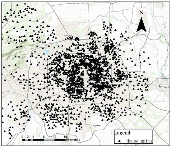
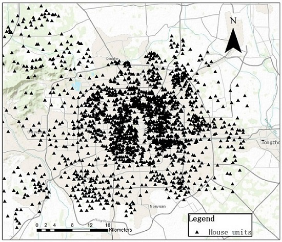
2. Study Area and Experimental Data

As the process of open reform in China moves forward, it has led to typical real estate market-based patterns in the metropolitan area. The hedonic real estate model is used to identify the contribution of the characteristics of a house (or other residence) to its purchase price [23,24,25,26,27,28]. Those characteristics can be divided into three general classes: structural attributes (house age, number of bedrooms, presence of a garage, etc.), locational attributes (these vary between properties and include good transportation links, accessibility to shops and services, proximity to downtown, etc.) and neighborhood attributes (population density, unemployment, measures of social stress, etc.). Some machine learning methods have been introduced to estimate house prices [29,30].

Houses are places for people to live or work; they constitute a main space for human activities. Clusters of houses connected by roads or paths form a community [9]. Therefore, it is reasonable to consider the accessibility relationships underlying a real estate market. Geographical accessibility comprises both accessibility and proximity. The availability of points of interest (POIs) through geographic services, such as Baidu, has made it possible to calculate road-network distances between residential plots and POIs, which can be particularly important in cities where driving is the dominant transportation modality. Network distances may provide a small improvement over the use of straight line distance metrics, particularly within urban areas. Although these distance metrics are an improvement on yet simpler models of distance, they remain somewhat unrealistic because they do not account for traffic congestion, which can alter the duration of a trip. However, it is possible to generate more accurate network travel cost metrics using detailed data on transportation infrastructure by accounting for the role of posted speed limits, traffic congestion, and so on.

This paper describes a case study carried out using housing price data observed in the urban area of Beijing, China. An overview of the variables involved in housing prices is shown in

Table 1. Variables used to predict housing prices in Beijing, China.

Abbreviation	Description	Minimum	Mean	Maximum
LnPrice	Log of the sales transaction price of the house	3.807	6.071	10.309
Structural Covariates
LnPlotRatio	Log of the plot ratio of houses	−4.605	0.679	2.303
LnGreenRatio	Log of the green ratio	−5.809	−1.162	−0.116
LnFloorArea	Log of the total floor area	2.303	4.532	7.507
LnPropertyFee	Log of the property management fee	−0.693	0.346	4.060
Temporal Covariates
Age	Age of the building at the time of sale (1980–2015)	1	23	30
Neighborhood Covariates
${\text{LnEucD}}_{\text{PriSchool}}$	Log of the Euclidean distance to the nearest primary school	0.499	6.393	16.322
${\text{LnEucD}}_{\text{ShoppingMall}}$	Log of the Euclidean distance to the nearest shopping mall	2.153	5.752	16.342
${\text{LnTD}}_{\text{PriSchool}}$	Log of the travel distance to the nearest primary school	1.386	6.462	12.701
${\text{LnTD}}_{\text{ShoppingMall}}$	Log of the travel distance to the nearest shopping mall	1.946	6.203	12.738

. A total of 1961 residential houses are included in the study; their geolocations are shown in Figure 1. The study data were provided by the National Bureau of Statistics. We extracted structural, neighborhood, and temporal variables to explain the variations in house prices.

The dependent variable is the logarithmically-transformed sales price (lnp) of the house. Unit prices are calculated in RMB. The structural characteristics of each house are described by four covariates. The plot ratio, also called floor area ratio, is the ratio of a building’s total floor area (gross floor area) to the size of the piece of land upon which it is built [31]. For example, in case of a land area of 100 m² and a floor area ratio of 300%, a building with maximum floor area of 300 m² can be constructed. The plot ratio is logarithmically transformed as LnPlotRatio. The green ratio is the ratio of green space to the entire plot area. The green ratio is logarithmically transformed as LnGreenRatio. The floor area of the house (in m²) is logarithmically transformed as LnFloorArea. The management fee of the property (in RMB/m²) is logarithmically transformed as LnPropertyFee. The temporal variable is the age of the building at the time of its last sale (in year). We calculate the Euclidean distance from each residential plot to the nearest primary school and shopping mall (${\text{LnEucD}}_{\text{PriSchool}}$, ${\text{LnEucD}}_{\text{ShoppingMall}}$), as well as the travel distance from each residential plot to the nearest primary school and shopping mall (${\text{LnTD}}_{\text{PriSchool}}$, ${\text{LnTD}}_{\text{ShoppingMall}}$).

Multicollinearity is investigated using the diagnostic tools of the variance inflation factor (VIF), condition index and variance-decomposition proportions [32]. VIF is defined as measuring the multicollinearity of a variable with the other independent variables in the analysis, and it is connected directly to the variance of the regression coefficient associated with this independent variable. The VIF value quantifies how much the variance is inflated by the existence of correlation among the explanatory variables in the model—in other words, VIF values are indicators for the severity of multicollinearity. A VIF value of 1 means that there is no correlation among the explanatory predictor and the remaining variables, while a VIF value greater than 10 means that that explanatory variable should be eliminated. Belsley suggests using condition indexes greater than or equal to 30 and variance proportions greater than 0.50 for each variance component as an indication of collinearity in a regression model [33,34]. In this study, the VIF values of the explanatory covariates are less than 10, and the condition indexes of all explanatory covariates and the intercept are less than 30.

3. Methods

3.1. Geographically Temporal Weighted Regression Model

The GWR approach is a spatially varying coefficient regression model [35,36,37]. Huang et al. developed a GTWR model to address spatial and temporal non-stationarity issues simultaneously by incorporating temporal effects into the GWR model [9]. To effectively delineate the spatio-temporal quantitative relationship between dependent and independent variables, a GTWR model with Euclidean and travel distance was developed to improve the estimation accuracy.

The GTWR model can be expressed as:

$$y_i={\beta }_0\left(u_i,v_i,t_i\right)+{{\displaystyle \sum }}_{k=\mathbf{1}}^p{\beta }_k\left(u_i,v_i,t_i\right)X_{ik}+{\epsilon }_i, i=1,2,\cdots ,n,$$

(1)

where $\left(u_i,v_i,t_i\right)$ epresents the given coordinate of a point $i$ in a space $\left(u_i,v_i\right)$ at time $t_i$; ${\beta }_0\left(u_i,v_i,t_i\right)$ represents the intercept value; and ${\beta }_k\left(u_i,v_i,t_i\right)$ represents a set of values for the number $p$ of parameters at point $i$. The random error conforming to a normal distribution is denoted by ${\epsilon }_i$, ${\epsilon }_i\sim N\left(0,{\sigma }^2\right)$. There is no correlation in random error between different points: $\text{Cov}\left({\epsilon }_i,{\epsilon }_j\right)=0\left(i\ne j\right)$.

The regression parameter ${\widehat{\beta }}_i$ at point $i$ can be calculated using the least squares model, as follows:

$${\widehat{\beta }}_i\left(u_i,v_i,t_i\right)={\left(X^{\prime }W\left(u_i,v_i,t_i\right)X\right)}^{-1}{X}^{\prime }W\left(u_i,v_i,t_i\right)y_i.$$

(2)

The fitted value $\widehat{y}$ is:

$$\widehat{y}=\left[\begin{array}{c}{\widehat{y}}_1\\ {\widehat{y}}_2\\ \cdots \\ {\widehat{y}}_n\end{array}\right]=\left[\begin{array}{c}{X}_1{\left(X^{\prime }W\left(u_1,v_1,t_1\right)X\right)}^{-1}{X}^{\prime }W\left(u_1,v_1,t_1\right)\\ X_2{\left(X^{\prime }W\left(u_2,v_2,t_2\right)X\right)}^{-1}{X}^{\prime }W\left(u_2,v_2,t_2\right)\\ \cdots \\ X_n{\left(X^{\prime }W\left(u_n,v_n,t_n\right)X\right)}^{-1}{X}^{\prime }W\left(u_n,v_n,t_n\right)\end{array}\right]y,$$

(3)

where the weighting matrix $W\left(u_i,v_i,t_i\right)$ is based on the distances between the regression point i and the data points around it. An adaptive kernel function is adopted and an optimum spatial kernel bandwidth is achieved for this study area. The Gaussian function is the most commonly used weighting function:

$$W_{ij}=\text{exp}\left(-\frac{d_{ij}^2}{h^2}\right),$$

(4)

where $h$ is a nonnegative parameter known as bandwidth that produces a decay of influence relative to the distance between the locations i and j. The spatial, temporal, and spatio-temporal distances between location i and j are as follows:

$$\{\begin{array}{c}{\left(d_{ij}^S\right)}^2={\left(u_i-u_j\right)}^2+{\left(v_i-v_j\right)}^2\\ {\left(d_{ij}^T\right)}^2={\left(t_i-t_j\right)}^2\\ {\left(d_{ij}^{ST}\right)}^2={\phi }^S\left[{\left(u_i-u_j\right)}^2+{\left(v_i-v_j\right)}^2\right]+{\phi }^T{\left(t_i-t_j\right)}^2\end{array}.$$

(5)

Here, ${\phi }^S$ is the scale factor of spatial distance, while ${\phi }^T$ stands for the scale factor of temporal distance:

$$\begin{array}{cc}\hfill W_{ij}& =\text{exp}\left\{-\left(\frac{{\phi }^S\left[{\left(u_i-u_j\right)}^2+{\left(v_i-v_j\right)}^2\right]+{\phi }^T{\left(t_i-t_j\right)}^2}{h_{ST}^2}\right)\right\}\hfill \\ & =\text{exp}\left\{-\left(\frac{{\left(d_{ij}^S\right)}^2}{h_S^2}+\frac{{\left(d_{ij}^T\right)}^2}{h_T^2}\right)\right\}\hfill \\ & =\text{exp}\left\{-\frac{{\left(d_{ij}^S\right)}^2}{h_S^2}\right\}\times \text{exp}\left\{-\frac{{\left(d_{ij}^T\right)}^2}{h_T^2}\right\}\hfill \\ & =W_{ij}^S\times W_{ij}^T\hfill \end{array},$$

(6)

where $h_{ST}$, $h_T$, and $h_S$ are the parameters of the spatio-temporal, spatial, and temporal bandwidths, respectively, and $h_S^2=h_{ST}^2/{\phi }^S$ and $h_T^2=h_{ST}^2/{\phi }^T$. The optimal spatial bandwidth $h_S$ is achieved by the optimization technique using the GWR model.

According to Equation (2), there is no influence on the estimation of coefficients when the kernel function is multiplied by a constant. The kernel function is determined by the distance and bandwidth. Therefore, the spatio-temporal distance $D_{ij}^{ST}$ could be written as follows:

$${\left(D_{ij}^{ST}\right)}^2=\frac{{\left(d_{ij}^{ST}\right)}^2}{{\phi }^S}=\left[{\left(u_i-u_j\right)}^2+{\left(v_i-v_j\right)}^2\right]+\mathsf{\tau }{\left(t_i-t_j\right)}^2,$$

(7)

where $\mathsf{\tau }=\frac{{\phi }^T}{{\phi }^S}$. The purpose of the spatio-temporal parameter $\mathsf{\tau }$ is to enlarge/reduce the temporal effect to match the spatial distance. To reduce the number of parameters and the computational complexity, set ${\phi }^S=1$; then, there is only one unknown parameter, $\mathsf{\tau }$. The spatio-temporal weight function can be constructed as follows:

$$\overline{W_{ij}}=\text{exp}\left(-\frac{D_{ij}^2}{h_{ST}^2}\right)=W_{ij}/{\phi }^S.$$

(8)

If the predicted value of $y_i$ from GTWR is denoted by ${\widehat{y}}_i\left(\mathsf{\tau }\right)$, the sum of the squared error can be written as follows:

$$\text{CV}\left(\mathsf{\tau }\right)={\displaystyle \sum }_i{\left(y_i-{\widehat{y}}_{\ne i}\left(\mathsf{\tau }\right)\right)}^2.$$

(9)

The spatio-temporal parameter $\mathsf{\tau }$ is achieved automatically with an optimization technique by minimizing Equation (9) in terms of goodness-of-fit statistics.

The AIC contains a penalty for the complexity of the model and provides a measure of the information distance between the fitted model and the unknown “true” model. As a general rule, improvements in the AIC less than 3 in value could easily arise as a result of sampling error, whereas values greater than 3 are more likely to be due to a genuine difference in models [3,8]. The AIC is expressed as:

$$\text{AIC}=2n\text{ln}\left(\widehat{\sigma }\right)+n\text{ln}\left(2\pi \right)+n+\text{tr}\left(S\right),$$

(10)

where n is the sample size; $\widehat{\sigma }$ is the estimated standard deviation of the error term; and tr(S) denotes the trace of the hat matrix $S$. The hat matrix $S$ is the projection matrix from the observed y to the fitted $\widehat{y}$ where each row $s_i$ of the hat matrix is:

$$s_i=X_i{\left(X^T{W}_{i}X\right)}^{-1}{X}^T{W}_i.$$

(11)

where $X_i$ is its i-th row of the matrix of explanatory variables $X$.

3.2. Measuring Travel Distance on a Beijing Road Network

To calibrate the GWR and GTWR models, the travel distance is used in both parts. As described by Lu and Curriero [8,9,38], the methods utilize non-Euclidean distances between residential plots. However, these methods do not consider the distance explanatory variables (i.e., the distance to the primary school or shopping mall). In this paper, the distances between residential plots are calculated using the travel distance. We also use travel distance instead of Euclidean distance as the distance metric to the nearest primary school and shopping mall. Travel distance is acquired from the Baidu Map API (the Route API), which, given starting and destination points, provides travel distance as a web service using the HTTP protocol. Two travel distance matrices are constructed and stored in a MySQL database (https://www.mysql.com). First, there are a total of 1961 residential plots; therefore, a two-dimensional $1961\times 1961$ matrix for travel distances between residential plots was constructed and stored in the MySQL database. Second, there are 971 primary schools and 3983 shopping malls in the study area; therefore, a two-dimensional $1961\times 2$ matrix for travel distances between residential plots to the nearest primary schools and shopping malls was constructed and stored to prepare for their invocation in the method.

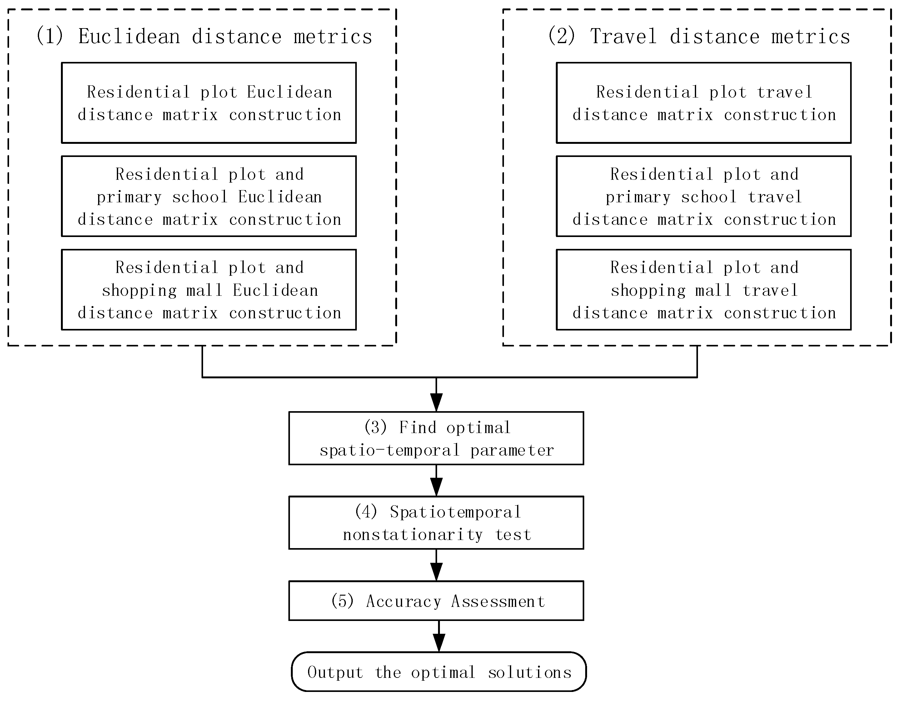
3.3. The Proposed Algorithm Flow

The flow of the proposed approach is shown in Figure 2. The steps of the proposed algorithm are as follows:

(1) Construct Euclidean distance matrices: Construct the residential plot to residential plot, residential plot to primary school, and residential plot to shopping mall Euclidean distance matrices.

(2) Construct travel distance matrices: Construct the residential plot to residential plot, residential plot to primary school, and residential plot and shopping mall travel distance matrices.

(3) Find the optimal spatio-temporal parameter, $\mathsf{\tau }$, which is used to harmonize the different spatial and temporal units. Equation (9) implements a validation process to achieve the optimal spatio-temporal parameter $\mathsf{\tau }$ in terms of goodness-of-fit.

(4) Calculate the response variable fitted value: Compute the fitted value $\widehat{y}$ according to Equation (3).

(5) Accuracy assessment: The $R^2$ and AIC statistics are selected to assess the accuracy of the proposed approach.

4. Experimental Results and Comparisons

In this section, the spatial and temporal heterogeneities were first tested using statistical hypotheses. Then, we performed regressions using both the traditional GWR and the proposed GTWR model, respectively, for the housing data. For comparison purposes, two different GWR-based approaches, GWR and GTWR with Euclidean and travel distance, were also implemented. All methods were tested against the same dataset, and we evaluated their goodness of fit in terms of the $R^2$ and AIC criteria.

4.1. Spatial and Temporal Heterogeneity Test of Significance

The statistical value proposed by Leung has been constructed to explain the spatial variation of the estimated values of parameters ${\beta }_i$ (i = 1, 2, ..., n) [39]. A test can be carried out by comparing the p-values against a threshold significance level, for example, 0.05. When a p-value is less than 0.05, the null hypothesis is rejected; otherwise, it is accepted.

Table 2. Nonstationarity of parameters in the GWR models.

Parameter	Euclidean Distance		Travel Distance
	F value	p-value	F value	p-value
Intercept	6.398	<0.001 *	9.858	<0.001 *
LnPlotRatio	1.140	0.178	1.718	<0.001 *
LnGreenRatio	5.032	<0.001 *	7.772	<0.001 *
LnFloorArea	1.551	<0.001 *	2.619	<0.001 *
LnPropertyFee	1.040	0.389	1.542	0.083
${\text{LnEucD}}_{\text{PriSchool}}$	1.453	0.012 *	1.485	<0.001 *
${\text{LnEucD}}_{\text{ShoppingMall}}$	1.132	0.190	1.771	<0.001 *
Age	1.435	0.007 *	2.477	<0.001 *

* The statistically significant values at the 5% level.

lists the F-statistic value of each variable and its corresponding p-value in the GWR models, and

Table 3. Nonstationarity of parameters in the GTWR models.

Parameter	Euclidean Distance		Travel Distance
	F value	p-value	F value	p-value
Intercept	5.686	<0.001 *	3.275	<0.001 *
LnPlotRatio	2.844	<0.001 *	3.166	<0.001 *
LnGreenRatio	1.899	<0.001 *	3.057	<0.001 *
LnFloorArea	4.111	<0.001 *	2.653	<0.001 *
LnPropertyFee	1.864	0.065	2.283	0.004 *
${\text{LnEucD}}_{\text{PriSchool}}$	1.910	<0.001 *	2.246	<0.001 *
${\text{LnEucD}}_{\text{ShoppingMall}}$	3.103	<0.001 *	2.822	<0.001 *
Age	12.882	<0.001 *	10.490	<0.001 *

* The statistically significant values at the 5% level.

lists the F-statistic value of each variable and its corresponding p-value in the GTWR models. The statistically significant values at the 5% level are marked with an asterisk (*). As Table 2 shows, the parameters Intercept, LnPlotRatio, LnGreenRatio, LnFloorArea, ${\text{LnEucD}}_{\text{PriSchool}}$, and age have significant spatial variation in the GWR model using Euclidean distance. The variable LnPropertyFee does not have spatial variation in the GWR with either the Euclidean or travel distance model or in the GTWR with the Euclidean model, but LnPropertyFee does show significant spatial variation in the GTWR with the travel distance model.

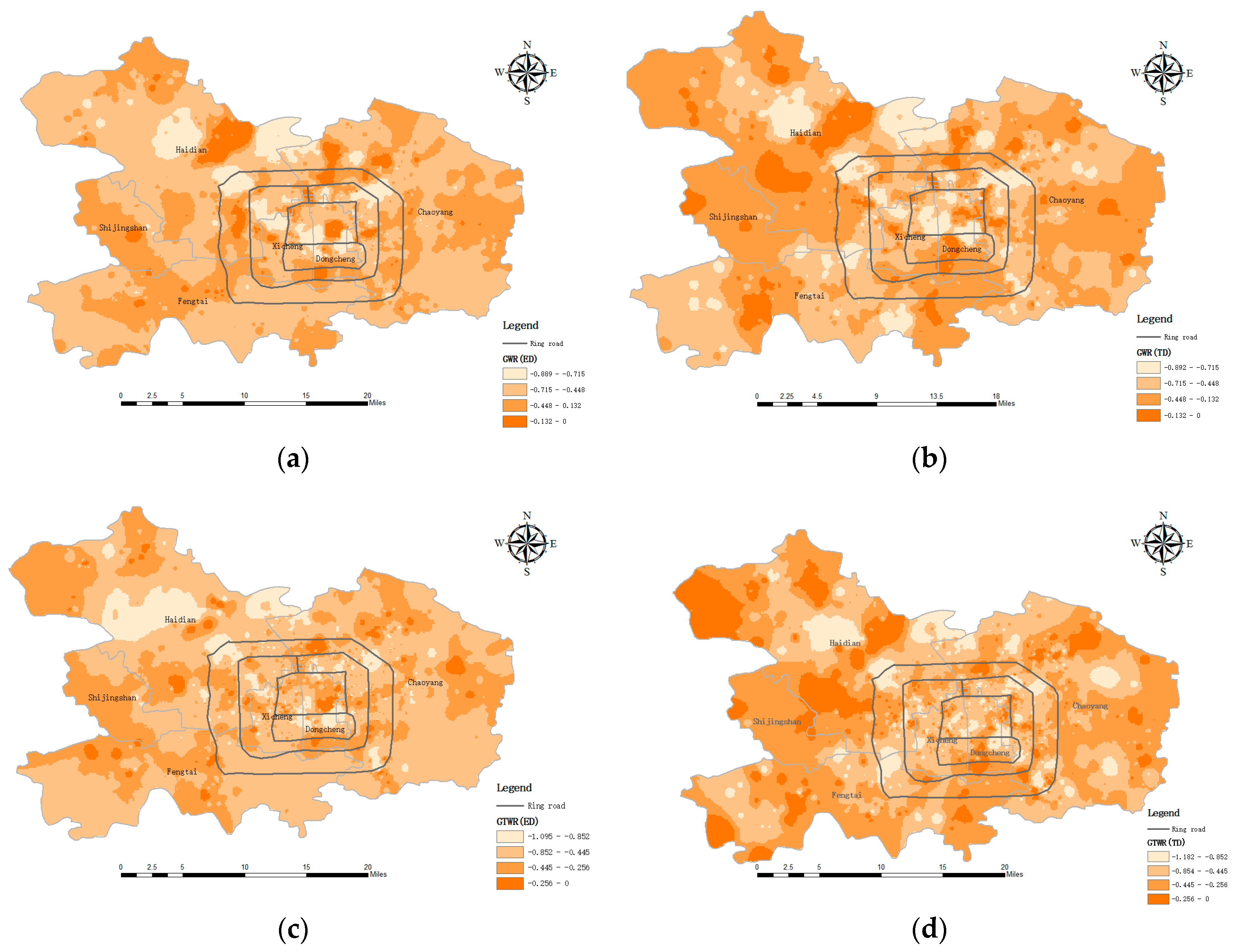
4.2. Comparison of the GTWR and GWR Models with Euclidean and Travel Distance Metrics

Summaries of the GWR coefficients estimation with Euclidean and travel distance, including the minimum (Min), lower quartile (LQ), median (Med), upper quartile (UQ), and maximum (Max) are presented in

Table 4. GWR coefficients estimate summaries with Euclidean distance.

Parameter	Min	LQ	Med	UQ	Max
Intercept	−12.158	0.055	1.237	2.327	15.63
LnPlotRatio	−1.209	−0.056	−0.004	0.047	1.607
LnGreenRatio	−14.58	−0.282	0.223	0.838	8.08
LnFloorArea	0.161	0.833	0.979	1.126	2.013
LnPropertyFee	−7.734	−0.104	1.9549	0.128	30.79
${\text{LnEucD}}_{\text{PriSchool}}$	−0.889	−0.512	−0.401	−0.165	−0.015
${\text{LnEucD}}_{\text{ShoppingMall}}$	−1.294	−0.055	0.013	0.088	0.802
Age	−0.42	−0.006	0.01	0.028	0.37

and

Table 5. GWR coefficients estimate summaries with travel distance.

Parameter	Min	LQ	Med	UQ	Max
Intercept	−9.535	0.023	1.221	2.348	15.074
LnPlotRatio	−0.58	−0.054	−0.003	0.047	0.913
LnGreenRatio	−6.675	−0.291	0.251	0.877	6.332
LnFloorArea	0.161	0.834	0.98	1.127	1.958
LnPropertyFee	−6.542	−0.104	1.085	0.132	21.21
${\text{LnEucD}}_{\text{PriSchool}}$	−0.892	−0.554	−0.410	−0.218	−0.018
${\text{LnEucD}}_{\text{ShoppingMall}}$	−0.753	−0.062	0.01	0.093	0.875
Age	−0.32	−0.006	0.009	0.026	0.236

. Summaries of the GTWR coefficients estimation with Euclidean and travel distance are reported in

Table 6. GTWR coefficients estimate summaries with Euclidean distance.

Parameter	Min	LQ	Med	UQ	Max
Intercept	−5.04	0.376	1.283	2.172	7.249
LnPlotRatio	−0.291	−0.04	−0.001	0.037	0.595
LnGreenRatio	−3.422	−0.194	0.201	0.594	4.162
LnFloorArea	0.161	0.883	1.004	1.134	1.546
LnPropertyFee	−2.131	−0.075	0.031	0.144	7.056
${\text{LnEucD}}_{\text{PriSchool}}$	−1.095	−0.711	−0.561	−0.292	−0.012
${\text{LnEucD}}_{\text{ShoppingMall}}$	−1.2	−0.038	0.013	0.068	0.454
Age	−0.091	−0.002	0.005	0.014	0.107

and

Table 7. GTWR coefficients estimate summaries with travel distance.

Parameter	Min	LQ	Med	UQ	Max
Intercept	−3.468	0.331	1.261	2.134	7.983
LnPlotRatio	−0.262	−0.039	−0.002	0.035	0.588
LnGreenRatio	−3.394	−0.169	0.215	0.636	3.737
LnFloorArea	0.161	0.886	1.005	1.138	1.59
LnPropertyFee	−2.238	−0.07	0.032	0.141	7.309
${\text{LnEucD}}_{\text{PriSchool}}$	−1.182	−0.644	−0.412	−0.258	−0.005
${\text{LnEucD}}_{\text{ShoppingMall}}$	−1.009	−0.039	0.013	0.066	0.447
Age	−0.083	−0.002	0.005	0.014	0.116

. When using the GWR and GTWR models with Euclidean and travel distance, ${\text{LnEucD}}_{\text{PriSchool}}$ is negatively correlated with house prices, as shown in Table 4. In other words, as the distance to the nearest primary school increases, the house price decreases. In contrast, LnFloorArea is positively correlated with house prices: the larger the living area is, the higher the house price is. However, there is no significant correlation between the variable ${\text{LnEucD}}_{\text{ShoppingMall}}$ and house prices since the coefficients of ${\text{LnEucD}}_{\text{ShoppingMall}}$ have both positive and negative values; therefore, shopping malls are not a major factor influencing house prices; however, this result occurred in this study because shopping malls are both common and relatively uniformly distributed in Beijing in the study area.

The F-test was implemented to compare with the improved sum of squares accounted for by the GWR and GTWR with Euclidean and travel distance metrics. These comparisons can be expressed in the form of an analysis of variance (ANOVA) table to compare the residual mean squares for these models, as reported in

Table 8. ANOVA comparison between GWR and GTWR with Euclidean and travel distance.

Models	RSS	DF	MS	F-test	p-value	R2	AIC
OLS	465.0	8	58.12	-	-
GWR(ED)	278.6	1787.5	0.16	1.9	0	0.724	1750.305
GWR(TD)	265.2	1778.3	0.15	2.2	0	0.737	1659.183
GTWR(ED)	243.2	1768.9	0.14	2.3	0	0.759	1483.361
GTWR(TD)	218.8	1755.6	0.13	2.9	0	0.783	1276.761
GWR(TD)/GWR(ED) Improvement	13.4	9.2	1.46	-	-	0.013	91.122
GTWR(TD)/GTWR(ED) Improvement	24.3	13.3	1.83	-	-	0.024	206.6
GTWR(TD)/GWR(TD) Improvement	46.3	22.7	2.04	-	-	0.046	382.422

. In this table, the second column lists the residual sum of squares (RSS) of the models and the improvement of one model compared to another. The third column lists the degrees of freedom (DF) for each model, and the fourth shows the mean squared error (MS). The fifth and sixth columns show the F statistic and its corresponding significance level. The R² and AIC measurements are also listed in Table 8.

As Table 8 shows, when using the GWR model with travel distance (TD) and ED (Euclidean distance), RSS improves by 13.4, MS improves by 1.46, $R^2$ improves by 0.013, and AIC improves by 91.122. In contrast, when using the GTWR and the GWR model with TD, RSS improves by 46.3, MS improves by 2.04, $R^2$ improves by 0.046, and AIC is reduced by 382.422. According to Fotheringham [40], a “serious” difference between the two models is generally regarded as one in which the difference in AIC values between the models is greater than three. The GTWR model with TD achieved both the maximum $R^2$ value and the minimum RSS, AIC value and, consequently, obtained the best performance.

The models’ performances and their spatio-temporal nonstationarity were explored visually by mapping the local coefficient estimates of the variable ${\text{LnEucD}}_{\text{PriSchool}}$. The maps in Figure 3 show the distribution of each individual coefficient.

As the maps in Figure 3 show, house prices are more strongly influenced in the metropolitan areas within the outer ring road of Beijing than in the suburban areas. Compared with primary schools in the suburban areas, primary schools in the metropolitan areas have excellent faculties and educational facilities. Therefore, house prices are influenced much more significantly by primary school proximity in the metropolitan areas than in the suburban areas. This result shows that it is critical for planning departments to arrange the locations of primary schools carefully to boost the sustainable development of the real estate industry.

Some exceptions can be found. For example, in the northwest portion of the suburban areas; the variable ${\text{LnEucD}}_{\text{PriSchool}}$ shows a significant negative correlation. This occurs because the area is home to a beautiful tourist spot named the Summer Palace, whose beauty and proximity influences nearby house prices.

5. Conclusions

This study analyzed data reflecting the spatial and temporal heterogeneity of house prices. The GWR and GTWR models used in the study were built based on house price data from 1980 to 2016. The performances of these two types of models were then compared based on $R^2$ and AIC. This article demonstrates that the GTWR model, which considers travel distance, is a more efficient approach for testing spatial and temporal nonstationarity in Beijing.

First, the GTWR model performs better than the GWR model with Euclidean and travel distance metrics. After spatial and temporal nonstationarity tests, the GTWR model can account for the spatial and temporal variations that exist in the house prices. Second, the GTWR performs better when using travel distance than when using Euclidean distance. This is because, in real life, people assess distances between their residential plots, primary schools, and shopping malls not by planar distance, but by distance when traveling along the road network. Third, the GTWR model revealed that distance to the nearest primary school plays an important negatively-correlated role in determining house prices in Beijing.

Although the present study demonstrates the utility of GTWR models with Euclidean and travel distance metrics for understanding specific location and temporal relationships between house prices and explanatory variables, some critical questions remain to be answered. This paper considered only spatial and temporal heterogeneity, but in the real world, some explanatory variables vary with spatial locations, whereas others do not. In future studies, we will focus on an MGTWR model to estimate house prices. Furthermore, this paper considers only the spatio-temporal heterogeneity and ignores spatial autocorrelation issues. More attention should be paid to the geographically- and temporally-weighted autoregressive model.

References

1. Tobler, W.R. A computer movie simulating urban growth in the Detroit region. Econ. Geogr. 1970, 46, 234–240. [Google Scholar] [CrossRef]
2. Griffith, D.A. Spatial-filtering based contributions to a critique of geographically weighted regression (GWR). Environ. Plan. A 2008, 40, 2751–2769. [Google Scholar] [CrossRef]
3. Brunsdon, C.; Fotheringham, A.S.; Charlton, M.E. Geographically weighted regression: A method for exploring spatial nonstationarity. Geogr. Anal. 1996, 28, 281–298. [Google Scholar] [CrossRef]
4. Farber, S.; Páez, A. A systematic investigation of cross-validation in GWR model estimation: Empirical analysis and Monte Carlo simulations. J. Geogr. Syst. 2007, 9, 371–396. [Google Scholar] [CrossRef]
5. Bitter, C.; Mulligan, G.F.; Dallérba, S. Incorporating spatial variation in housing attribute prices: A comparison of geographically weighted regression and the spatial expansion method. J. Geogr. Syst. 2007, 9, 7–27. [Google Scholar] [CrossRef] [Green Version]
6. Wei, C.H.; Qi, F. On the estimation and testing of mixed geographically weighted regression models. Econ. Modell. 2012, 29, 2615–2620. [Google Scholar] [CrossRef]
7. Helbich, M.; Brunauer, W.; Vaz, E.; Nijkamp, P. Spatial heterogeneity in hedonic house price models: The case of Austria. Urban Stud. 2014, 51, 390–411. [Google Scholar] [CrossRef]
8. Lu, B.; Charlton, M.; Fotheringhama, A.S. Geographically weighted regression using a non-euclidean distance metric with a study on London house price data. Procedia Environ. Sci. 2011, 7, 92–97. [Google Scholar] [CrossRef]
9. Lu, B.; Charlton, M.; Harris, P.; Fotheringham, A.S. Geographically weighted regression with a non-euclidean distance metric: A case study using hedonic house price data. Int. J. Geogr. Inf. Sci. 2014, 28, 660–681. [Google Scholar] [CrossRef]
10. Mcmillen, D.P.; Redfearn, C.L. Estimation, Interpretation, and Hypothesis Testing for Nonparametric Hedonic House Price Functions. Available online: http://lusk.usc.edu/sites/default/files/working_papers/wp_2007-1007.pdf (accessed on 11 August 2016).
11. Mcmillen, D.P.; Redfearn, C.L. Estimation and hypothesis testing for nonparametric hedonic house price functions. J. Reg. Sci. 2010, 50, 712–733. [Google Scholar] [CrossRef]
12. Bai, Y.; Wu, L.; Qin, K.; Zhang, Y.; Shen, Y.; Zhou, Y. A geographically and temporally weighted regression model for ground-level PM2.5 estimation from satellite-derived 500 m resolution AOD. Remote Sens. 2016, 8, 262. [Google Scholar] [CrossRef]
13. Huang, B.; Wu, B.; Barry, M. Geographically and temporally weighted regression for modeling spatio-temporal variation in house prices. Int. J. Geogr. Inf. Sci. 2010, 24, 383–401. [Google Scholar] [CrossRef]
14. Wrenn, D.H.; Sam, A.G. Geographically and temporally weighted likelihood regression: Exploring the spatiotemporal determinants of land use change. Reg. Sci. Urban Econ. 2014, 44, 60–74. [Google Scholar] [CrossRef]
15. Griffith, D.A. Spatial Autocorrelation: A Primer; Assn of Amer Geographers: Washington, DC, USA, 1987. [Google Scholar]
16. Wu, B.; Li, R.; Huang, B. A geographically and temporally weighted autoregressive model with application to housing prices. Int. J. Geogr. Inf. Sci. 2014, 28, 1186–1204. [Google Scholar] [CrossRef]
17. Ahlfeldt, G. If Alonso was right: Modeling accessibility and explaining the residential land gradient. J. Reg. Sci. 2011, 51, 318–338. [Google Scholar] [CrossRef]
18. Apparicio, P.; Abdelmajid, M.; Riva, M.; Shearmur, R. Comparing alternative approaches to measuring the geographical accessibility of urban health services: Distance types and aggregation-error issues. Int J. Health Geogr. 2008, 7. [Google Scholar] [CrossRef] [PubMed] [Green Version]
19. Mcgrail, M.R.; Humphreys, J.S. Measuring spatial accessibility to primary care in rural areas: Improving the effectiveness of the two-step floating catchment area method. Appl. Geogr. 2009, 29, 533–541. [Google Scholar] [CrossRef]
20. Schuurman, N.; Bérubé, M.; Crooks, V.A. Measuring potential spatial access to primary health care physicians using a modified gravity model. Can. Geogr. 2010, 54, 29–45. [Google Scholar] [CrossRef]
21. Yiannakoulias, N.; Bland, W.; Svenson, L.W. Estimating the effect of turn penalties and traffic congestion on measuring spatial accessibility to primary health care. Appl. Geogr. 2013, 39, 172–182. [Google Scholar] [CrossRef]
22. Lu, B.; Charlton, M.; Brunsdon, C. The Minkowski approach for choosing the distance metric in geographically weighted regression. Int. J. Geogr. Inf. Sci. 2015, 30, 351–368. [Google Scholar] [CrossRef]
23. Selim, H. Determinants of house prices in Turkey: Hedonic regression versus artificial neural network. Expert Syst. Appl. 2009, 36, 2843–2852. [Google Scholar] [CrossRef]
24. Redfearn, C.L. How informative are average effects? Hedonic regression and amenity capitalization in complex urban housing markets. Reg. Sci. Urban Econ. 2009, 39, 297–306. [Google Scholar] [CrossRef]
25. Peterson, S.; Flanagan, A. Neural network hedonic pricing models in mass real estate appraisal. J. R. Estate Res. 2009, 31, 147–164. [Google Scholar]
26. Paez, A.; Long, F.; Farber, S. Moving window approaches for hedonic price estimation: An empirical comparison of modelling techniques. Urban Stud. 2008, 45, 1565–1581. [Google Scholar] [CrossRef]
27. Farber, S.; Yeates, M. A comparison of localized regression models in a hedonic house price context. Can. J. Reg. Sci. 2006, 29, 405–420. [Google Scholar]
28. Selim, S. Determinants of house prices in turkey: A hedonic regression model. Doğuş Üniversitesi Dergisi 2008, 9, 65–76. [Google Scholar]
29. Guan, J.; Zurada, J.; Levitan, A. An adaptive neuro-fuzzy inference system based approach to real estate property assessment. J. R. Estate Res. 2008, 30, 395–422. [Google Scholar]
30. Kuşan, H.; Aytekin, O.; Özdemir, İ. The use of fuzzy logic in predicting house selling price. Expert Syst. Appl. 2010, 37, 1808–1813. [Google Scholar] [CrossRef]
31. Barr, J.; Cohen, J.P. The floor area ratio gradient: New York City, 1890–2009. Reg. Sci. Urban Econ. 2014, 48, 110–119. [Google Scholar] [CrossRef]
32. Garcia, C.B.; Garcia, J.; Martin, M. Collinearity: Revisiting the variance inflation factor in ridge regression. J. Appl. Stat. 2015, 42, 648–661. [Google Scholar] [CrossRef]
33. Wheeler, D.; Tiefelsdorf, M. Multicollinearity and correlation among local regression coefficients in geographically weighted regression. J. Geogr. Syst. 2005, 7, 161–187. [Google Scholar] [CrossRef]
34. Wheeler, D.C. Diagnostic tools and a remedial method for collinearity in geographically weighted regression. Environ. Plan. A 2007, 39, 2464–2481. [Google Scholar] [CrossRef]
35. Páez, A.; Farber, S.; Wheeler, D. A simulation-based study of geographically weighted regression as a method for investigating spatially varying relationships. Environ. Plan. A 2011, 43, 2992–3010. [Google Scholar] [CrossRef]
36. Cho, S.; Lambert, D.M.; Kim, S.G.; Jung, S. Extreme coefficients in geographically weighted regression and their effects on mapping. GIsci. Remote Sens. 2009, 46, 273–288. [Google Scholar] [CrossRef]
37. Harris, R.; Dong, G.; Zhang, W. Using contextualized geographically weighted regression to model the spatial heterogeneity of land prices in Beijing, China. Trans. GIS 2013, 17, 901–919. [Google Scholar] [CrossRef]
38. Curriero, F.C. On the use of non-euclidean distance measures in geostatistics. Math. Geol. 2007, 38, 907–926. [Google Scholar] [CrossRef]
39. Leung, Y.; Mei, C.; Zhang, W. Statistical tests for spatial nonstationarity based on the geographically weighted regression model. Environ. Plan. A 2000, 32, 9–32. [Google Scholar] [CrossRef]
40. Fotheringham, A.S.; Brunsdon, C.; Charlton, M. Geographically weighted regression: The analysis of spatially varying relationships. Am. J. Agric. Econ. 2004, 86, 554–556. [Google Scholar]
Figure 1. Map of the study area.
Entropy 18 00303 g001
Figure 2. The flow of the proposed approach.
Entropy 18 00303 g002
Figure 3. Distance to primary school coefficients map over the study region: (a) GWR model with Euclidean distance; (b) GWR model with travel distance; (c) GTWR model with Euclidean distance; and (d) GTWR model with travel distance.
Entropy 18 00303 g003