Filters, Waves and Spectra

Abstract

Econometric analysis requires filtering techniques that are adapted to cater to data sequences that are short and that have strong trends. Whereas the economists have tended to conduct their analyses in the time domain, the engineers have emphasised the frequency domain. This paper places its emphasis in the frequency domain; and it shows how the frequency-domain methods can be adapted to cater to short trended sequences. Working in the frequency domain allows an unrestricted choice to be made of the frequency response of a filter. It also requires that the data should be free of trends. Methods for extracting the trends prior to filtering and for restoring them thereafter are described.

1. Introduction

Techniques of filtering have been employed in econometric analysis since the inception of the subject in the second quarter of the 20th century. Major advances in the linear filtering theory were achieved, subsequently, by engineers and mathematicians during and after the Second World War. These developments were largely in aid of military technology.

The notable contributions of Wiener [1941] (1949) and of Kolmogorov (1941a,1941b) were addressed, originally, to the problem of anti-aircraft fire control (see Guerlac 1947). The work of the Radar Laboratory of MIT (the Rad Lab), which operated from 1940 to 1945, formed the basis of the textbooks on signal processing that began to be published in the late 1950s; and its influence is still discernible in modern texts.

As soon as security permitted, the wartime work of the Rad Lab was published in 28 volumes by the McGraw-Hill Publishing Co. (New York), beginning with the survey volume of Ridenour (1947) and culminating in the combined index of Henney (1953).

These advances were succeeded by a revolution in digital communications, which has involved the conversion of continuous-time formulations to their discrete-time counterparts. The developments were assisted by the discovery of a variety of computational algorithms, which have come to be known collectively as the fast Fourier transform or as the FFT. A major contribution was the algorithm of Cooley and Tukey (1965).

The mature state of the art in digital signal processing was summarised in the texts of Rabiner and Gold (1975) and of Oppenheim and Schafer (1975) and in the survey paper of Kailath (1974).

In the process of the digital revolution, the theory of signal processing has become more appropriate to econometric applications that depend on sampled data. Nevertheless, it is only recently that economists have begun to pay attention to the engineering literature; and their outlook remains significantly different from that of the engineers.

The engineering literature is concerned, primarily, with the frequency characteristics of the signals that are the subjects of the analysis. A frequency-domain analysis presupposes that the signals can be represented by linear combinations of trigonometric or complex exponential functions. These are perpetual periodic or circular functions. Therefore, the resulting theory is appropriate to stationary signals of an indefinite duration that are devoid of trends.

Economists, by contrast, are concerned, primarily, with data sequences of a limited duration that often manifest significant trends both in their levels and in the amplitudes of their fluctuations. In addition, the economists have tended to conduct their analyses in the time domain as opposed to the frequency domain. The notable exceptions have been the books of Granger and Hatanaka (1964) and of Fishman (1969). Moreover, the adaptation of the engineering theory to the circumstances of trended data sequences of limited duration has continued to be problematic.

This paper will begin by expounding a frequency-domain approach that relies on the concepts of Fourier analysis. It will demonstrate the connection between the discrete-time and continuous-time formulations and it will show that, notwithstanding the fixity of the sampling intervals in econometric data, the rate of sampling can be varied whenever it is possible to reconstitute the continuous trajectory of a signal from its sampled values.

By resampling the data at a lesser rate, the spectral support of a data component of limited frequency can be expanded so that it extends over the full Nyquist interval that runs from zero frequency to a frequency of $\pi$ radians per sampling interval. This should enable the component to be represented successfully by an autoregressive moving-average (ARMA) model.

The paper will proceed to show how a variety of filters that have been conceived in the time domain can be usefully implemented by conducting the essential computations in the frequency domain. Working in the frequency domain will allow an unrestricted choice of the frequency response of the filter.

2. Sinc Function Interpolation and the Sampling Theorem

The data that are available for time-series analysis are usually obtained by sampling continuous processes at regular intervals. The observable frequencies are limited to a maximum of $\pi$ radians per sampling interval, which is described as the Nyquist frequency. Frequencies in excess of this value are confounded with their aliases the lie within the Nyquist interval of $[-\pi ,\pi ]$.

2.1. Aliasing

To illustrate the effect of aliasing, we may consider the case of a pure cosine wave of unit amplitude and zero phase displacement of which the frequency is $\omega \in [\pi ,2\pi ]$, so that $2\pi -\omega ={\omega }^{*}\in [0,\pi ]$. Let $t\in \{0,\pm 1,\pm 2,\dots \}$, which is to say that the samples are taken at unit intervals. Then,

$$\begin{array}{ccc}\hfill cos(\omega t)& =& cos\{(2\pi -{\omega }^{*})t\}\hfill \\ & =& cos(2\pi t)cos({\omega }^{*}t)+sin(2\pi t)sin({\omega }^{*}t)\hfill \\ & =& cos({\omega }^{*}t),\hfill \end{array}$$

(1)

which indicates that $cos(\omega t)$ and $cos({\omega }^{*}t)$, which is its alias, are observationally equivalent. The trigonometric functions are liable to be expressed in terms of complex exponential functions that have both positive and negative frequencies (see Equation (A1) in Appendix A).

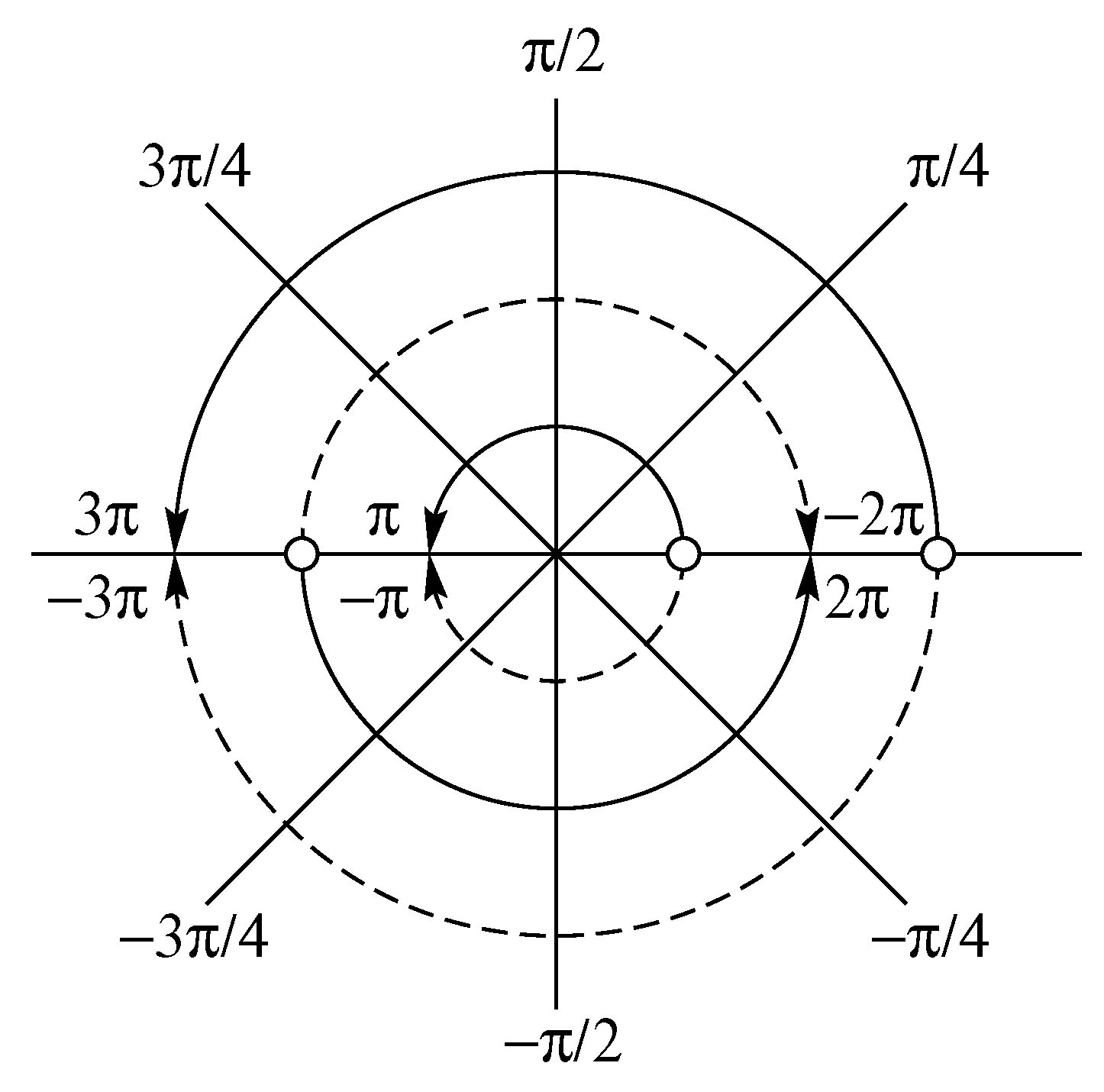
Within the sampled data, frequencies that lie beyond the Nyquist interval $[-\pi ,\pi ]$ are mapped into that interval by a process of circular wrapping. The interval $[-\pi ,\pi ]$ corresponds to the angles made with the positive horizontal axis by the radius of a circle. For positive frequencies $\omega >0$, the segment $[0,\omega ]$ is wrapped around the circle in an anticlockwise sense. The end of the wrapped segment marks the tip of a radius of which the angle ${\omega }^{*}$ is the alias of $\omega$. For a negative frequencies $\omega <0$, the segment $[\omega ,0]$ is wrapped around the circle in a clockwise sense.

The effect, for a positive frequency $\omega >0$, is that a multiple k of $2\pi$, which is the number of windings rounded to the nearest integer, is subtracted such that ${\omega }^{*}=\omega -k2\pi \in [-\pi ,\pi ]$, whereas, for negative frequencies, a multiple of $2\pi$ is added to produce the same effect. The following formula maps from the angles to their aliases:

$$\omega ⟶{\omega }^{*}=\left\{\begin{array}{c}\{(\omega +\pi )\mathrm{mod}2\pi \}-\pi \},\mathrm{if}\omega >0,\hfill \\ \{(\omega -\pi )\mathrm{mod}2\pi \}+\pi ,\mathrm{if}\omega <0.\hfill \end{array}\right.$$

(2)

The calculation can be made via the diagram of Figure 1.

A continuous trajectory may be derived from a sequence $\{y_t;t=0,\pm 1,\pm 2,\dots \}$, sampled from a continuous absolutely integrable signal $y(t)$, by a method of kernel interpolation. A kernel $\varphi (t)$ is a continuous unimodal function of which the (absolute) values diminish with the distance from its centre at $t=0$ and which integrates to unity. The discrete impulses of the sequence may be replaced by kernel or scaling functions of the appropriate scales, of which the overlapping ordinates are summed at every point on the real line. The interpolated continuous function is

$$x(t)=\sum _{k=-\infty }^{\infty }{y}_k\varphi (t-k).$$

(3)

2.2. The Sampling Theorem

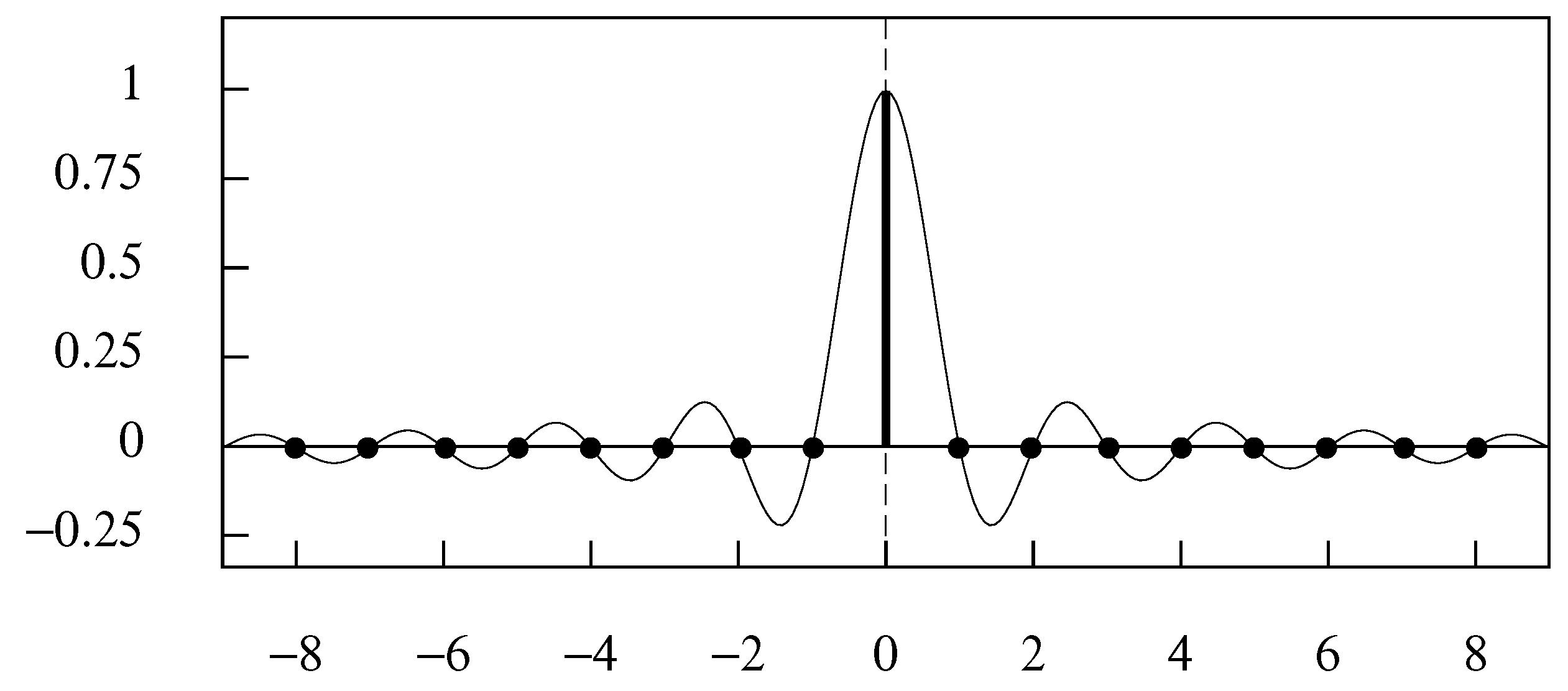
The mathematically ideal way to interpolate the sequence is to use the so-called sinc function kernel. A sinc function centred on k, which is the (inverse) Fourier transform of a rectangle in the frequency domain, is defined by

$${\varphi }_0(t-k)=\frac{1}{2\pi }{\int }_{-\pi }^{\pi }{e}^{\mathrm{i}\omega (t-k)}d\omega =\frac{e^{\mathrm{i}\pi (t-k)}-e^{-\mathrm{i}\pi (t-k)}}{2\pi \mathrm{i}(t-k)}=\frac{sin\{\pi (t-k)\}}{\pi (t-k)}.$$

(4)

The conversion of the complex exponential functions on the LHS of the equation to the trigonometric function on the RHS depends on Euler’s equations, which are displayed in Appendix A, where an account of the Fourier transform is also to be found. This sinc function, which is represented in Figure 2, may also be described, in the context of a wavelets analysis, as a scaling function.

The sinc function has a limiting frequency of $\pi$, and, provided that the frequencies in the original continuous function $x(t)$, from which a sequence $\{x_k;k=0,\pm 1,\pm 2,\dots \}$ has been sampled, are bounded by this value, then, as the Nyquist–Shannon sampling theorem indicates, a sinc-function interpolation will recover its trajectory exactly.

Let $x(t)$ be an absolutely integrable continuous function defined on the real line. Then, the Fourier integral transform gives rise to the following expressions in the time domain and the frequency domain:

$$x(t)=\frac{1}{2\pi }{\int }_{-\infty }^{\infty }\xi (\omega )e^{\mathrm{i}\omega t}d\omega ⟷\xi (\omega )={\int }_{-\infty }^{\infty }x(t)e^{-\mathrm{i}\omega t}dt.$$

(5)

However, if the frequencies are bounded by the Nyquist value of $\pi$, then there is a discrete-time Fourier transform

$$x(t)=\frac{1}{2\pi }{\int }_{-\pi }^{\pi }{\xi }^{\circ }(\omega )e^{\mathrm{i}\omega t}d\omega ⟷{\xi }^{\circ }(\omega )=\sum _{k=-\infty }^{\infty }{x}_k{e}^{-\mathrm{i}k\omega },$$

(6)

where $\{x_k;k=0,\pm 1,\pm 2,\dots \}$ is sampled at unit intervals from $x(t)$. Putting the RHS of (6) into the LHS and interchanging the order of integration and summation gives

$$x(t)=\frac{1}{2\pi }\sum _{k=-\infty }^{\infty }{x}_k\left\{{\int }_{-\pi }^{\pi }{e}^{\mathrm{i}\omega (t-k)}\right\}d\omega =\sum _{k=-\infty }^{\infty }{x}_k{\varphi }_0(t-k),$$

(7)

where ${\varphi }_0(t-k)$ is the sinc function of (4).

It should be observed that ${\xi }^{\circ }(\omega )$, which is described as the discrete-time Fourier transform of the sequence $\{x_k\}$, or, equally, as the spectrum of the sequence, is a continuous $2\pi$-periodic function of $\omega$. Moreover, if the sequence is real-valued, then ${\xi }^{\circ }(\omega )$ will be distributed symmetrically around zero in the interval $[-\pi ,\pi ]$, which enables the function to be represented by its values over the interval $[0,\pi ]$, which is the usual recourse.

The sampling theorem is attributable to several people, but it is most commonly attributed to Shannon (1949a, 1949b), albeit that Nyquist (1928) discovered the essential results at an earlier date.

Equation (7) of the Nyquist–Shannon sampling theorem represents an essential theoretical result, but it does not correspond to a practical way of creating a continuous trajectory from a finite sequence of values. The difficulty arises from the fact that $\{x_k;k=0,\pm 1,\pm 2,\dots \}$ is a doubly-infinite sequence and from the fact that each of the sinc function kernels is supported on the entire of the real line $\mathcal{R}=(-\infty ,\infty )$.

To interpolate a continuous function through a finite sequence of T equally spaced elements, the sinc function must be replaced by the Dirichlet kernel, which would result from wrapping the sinc function around a circle of circumference T and adding the overlying ordinates. However, an interpolation by Dirichlet kernels is equivalent to an ordinary Fourier interpolation (i.e., an interpolation via a Fourier synthesis). This is demonstrated in Section 4.5.

2.3. Orthogonal Bases and Wavelets

The sinc function is symmetric and idempotent such that

$${\varphi }_0(t)={\varphi }_0(-t)\mathrm{and}{\varphi }_0(t)={\int }_{-\infty }^{\infty }{\varphi }_0(t){\varphi }_0(t-\tau )d\tau .$$

(8)

The latter follows from the fact that the unit rectangle on $[-\pi ,\pi ]$, which is the counterpart of the sinc function in the frequency domain, is unaltered when squared, and from the fact that a modulation in the frequency domain—in this case a squaring—corresponds to a convolution in the time domain.

The two properties of (8) imply that ${\varphi }_0(t)$ is its own autocovariance function. Therefore, the condition that ${\varphi }_0(t)=0$ for $t\in \{\pm 1,\pm 2,\dots \}$, which is manifest in Figure 2, implies that the sequence $\{{\varphi }_0(t-k);k=0,\pm 1\pm 2,\dots \}$ constitutes an orthogonal basis for the set of all functions bounded in frequency by the Nyquist value of $\pi$ radians per unit (sampling) interval.

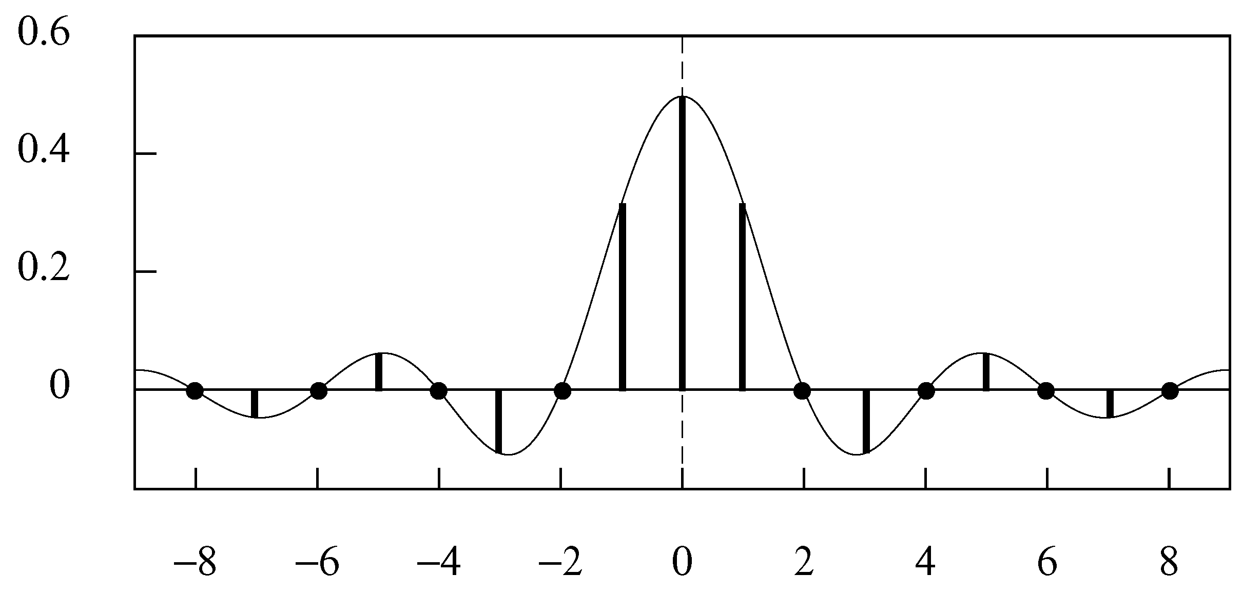
The sinc function kernel ${\varphi }_0(t)$ of Equation (4) is supported on the Nyquist frequency interval $[0,\pi ]$. A sinc function with a lesser frequency content can be used to create a smoother trajectory. The sinc function that is bounded in frequency by ${\omega }_c\le \pi$ and centred on $k=0$ is

$${\varphi }_c(t)=\frac{sin({\omega }_{c}t)}{\pi t}.$$

(9)

Figure 3 represents the function ${\varphi }_1(t)=sin(\pi t/2)/\pi t$ for which ${\omega }_c=\pi /2$. It will be seen that ${\varphi }_1(t)=0$ for $t\in \{\pm 2,\pm 4,\dots \}$; and it can be inferred that $\{{\varphi }_1(t-2k);k=0,\pm 1\pm 2,\dots \}$ constitutes an orthogonal basis for the set of all functions bounded in frequency by $\pi /2$ radians.

A function that contains the low-frequency content of $y(t)$, and which is therefore smoother, can be obtained by associating the half-frequency sinc functions to the elements of the sampled sequence $\{y_t;t=0,\pm 1,\pm 2\dots \}$ to form

$$x(t)=\sum _{k=-\infty }^{\infty }{y}_k{\varphi }_1(t-k).$$

(10)

The smoothing effect is by dint of the way in which the value of each discrete-time ordinate is dispersed more widely than in the case of the sinc function of (4), wherein ${\omega }_c=\pi$. To produce a smooth approximation to $y(t)$, it would be necessary to multiply the functions ${\varphi }_1(t-k)$ by 2 to ensure that they integrate to unity.

The complete information content of the function $x(t)$ will be conveyed by the sequence $\{x_{2t}=x(2t);t=0,\pm 1,\pm 2,\dots \}$ sampled from the continuous trajectory, less frequently, at intervals of two units. Whereas the discrete Fourier transform ${\sum }_k{x}_{k}exp\{-\mathrm{i}\omega k\}$ of the sequence $\{x_k\}$ will be nonzero only over the half interval $[-\pi /2,\pi /2]$, that of the subsampled sequence $\{x_{2k}\}$, which is ${\sum }_k{x}_{2k}exp\{-\mathrm{i}\omega 2k\}$, is liable to be nonzero over the entire Nyquist interval. Thus, whereas subsampling will compress the sequence, its effect in frequency-domain is to distend the spectrum.

The sinc function ${\varphi }_1(t)$ can be expressed in terms of the functions ${\varphi }_0(t-k)$, which provide an orthogonal basis for the set of functions bounded in frequency by $\pi$. Thus,

$${\varphi }_1(t)=\sum _k{g}_k{\varphi }_0(t-k),$$

(11)

where the coefficients $\{g_k={\varphi }_1(k);k=0,\pm 1,\pm 2,\dots \}$ are sampled from the function ${\varphi }_1(t)$ at unit intervals. The same relationship prevails between the functions ${\varphi }_{j+1}(t)$ and ${\varphi }_j(t)$, which are supported on the frequency intervals $[0,\pi /2^{j+1}]$ and $[0,\pi /2^j]$, respectively.

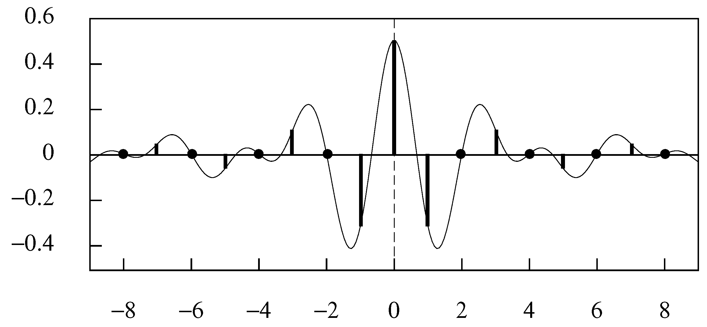
The sinc function ${\varphi }_1(t)=sin(\pi t/2)/\pi t$ is accompanied by a complementary wavelet function defined on the interval $[\pi ,-\pi /2]\cap [\pi /2,\pi ]=[\pi /2,-\pi /2]$, if one is considering the constituent complex exponential functions, or on the interval $[\pi /2,\pi ]$, if one is considering the trigonometric functions. The interval $[\pi /2,-\pi /2]$ contains the angles subtended by the left half of the unit circle centred on the origin of the complex plane. The wavelet is shown in Figure 4.

The wavelet can be expressed variously as

$$\begin{array}{c}\hfill \begin{array}{ccc}{\psi }_1(t)={\varphi }_0(t)-{\varphi }_1(t)& =& {\displaystyle \frac{1}{\pi t}\{sin(\pi t)-sin(\pi t/2)\}}\hfill \\ & =& {\displaystyle \frac{1}{\pi t}cos(\pi t)sin(\pi t/2).}\hfill \end{array}\end{array}$$

(12)

The final expression represents the effect of shifting the scaling function in frequency by $\pi$ radians, via a method of cosine modulation, whereby the frequency interval $[-\pi /2,\pi /2]$, which supports the scaling function, becomes the interval $[\pi /2,-\pi /2]$, which is the support of the wavelet. The effect of multiplying the sinc function by $cos(\pi t)=\{exp(\mathrm{i}\pi t)+exp(-\mathrm{i}\pi t)\}/2$ is to shift two copies of its frequency-domain rectangle from its centre at zero to centres of $\pi$ and $-\pi$, whereafter the copies are added and divided by 2. A generalised method of cosine modulation is described in Section 4.1.

The decomposition ${\varphi }_0(t)={\psi }_1(t)+{\varphi }_1(t)$ of the original sinc function at level 0 into a scaling function ${\varphi }_1(t)$ and a wavelet ${\psi }_1(t)$ at level 1 represent the first stage of a dyadic decomposition that can be applied to the succession of scaling functions of diminishing frequency content and of increasing dispersion, so as to create an orthogonal wavelets basis.

The wavelet ${\psi }_1(t)$ at level 1 can be expressed as a linear combination of the scaling functions at level 0. Thus, there is

$${\psi }_1(t)=\sum _k{h}_k{\varphi }_0(t-k),$$

(13)

which is similar to Equation (11). The scaling function and the wavelet at any level j are mutually orthogonal, since their frequency bands $[0,\pi /2^{j+1}]$ and $[\pi /2^{j+1},\pi /2^j]$ are virtually disjoint.

There are other scaling functions and their accompanying wavelets that can give rise to orthogonal dyadic decompositions. These functions tend to benefit from having finite supports in the time domain. However, a reduction of the dispersion in the time domain leads to an increased dispersion in the frequency domain, with the effect that the functions are no longer confined to their designated frequency bands.

A fuller account of wavelets analysis is available in many texts, amongst which the coupled volumes of Vetterli et al. (2014) and Kovačević et al. (2013), which are available on the web, give a comprehensive account of the theory. Another source at a high level of mathematical sophistication is the volume of Mallat (1998).

Wavelets analysis has many practical applications, of which the statistical applications are touched on in the paper of Abramovich et al. (2000). From the present point of view, wavelets analysis can be regarded as a synthesis of the discrete-time and the continuous-time analyses of signals.

3. Linear Filters

Let $\{{\varphi }_j=\varphi (j);j=0,\pm 1,\pm 2,\dots \}$ be a sequence sampled at unit intervals from the kernel function $\varphi (j)$. Then, the sequence $\{x_t=x(t);t=0,\pm 1,\pm 2,\dots \}$, sampled from the trajectory $x(t)$ of (3), can be generated by a discrete-time convolution such that

$$x_t=\sum _{k=-\infty }^{\infty }{y}_k{\varphi }_{t-k}=\sum _{k=-\infty }^{\infty }{\varphi }_k{y}_{t-k}.$$

(14)

This equation describes an operation of linear filtering applied to the sequence $\{y_t;t=0,\pm 1,\pm 2,\dots \}$.

The first expression on the RHS of (14), which corresponds to the expression of Equation (3) for kernel function interpolation, depicts a dispersion over time of the data ordinates. The second expression, which is the more usual one, depicts the operation of filtering as a matter of forming a moving average of the data.

In demonstrating the effects of the filter, it is helpful to consider the z-transforms of the various sequences. The data sequence $\{x_t;t=0,\pm 1,\pm 2,\dots \}$ is converted to a power series by associating $z^t$ to each element $x_t$ and by summing the resulting sequence. Thus,

$$\begin{array}{c}\hfill \begin{array}{ccc}{\displaystyle \sum _t{x}_t{z}^t}& =& {\displaystyle \sum _t\left\{\sum _j{\varphi }_j{y}_{t-j}\right\}{z}^t=\left\{\sum _j{\varphi }_j{z}^j\right\}\left\{\sum _t{y}_t{z}^t\right\},}\\ & & \mathrm{or}x(z)=\varphi (z)y(z).\end{array}\end{array}$$

(15)

The convolution operation of Equation (14) becomes an operation of polynomial multiplication in Equation (15). The z-transform $\varphi (z)$ of the filter coefficients is liable to be described as the transfer function of the filter.

The sequence $\{{\varphi }_j;j=0,\pm 1,\pm 2,\dots \}$ of the filter coefficients is also described as the impulse response of the filter, since ${\varphi }_j$ can be obtained from the equation ${\varphi }_j=\sum {\varphi }_k{\delta }_{j-k}$ when $\{{\delta }_{j-k}\}$, is an impulse sequence that has a unit where $k=j$ and zeros elsewhere.

3.1. The Gain and Phase Effects

The frequency response of the filter, which is a continuous function of the frequency $\omega \in [-\pi ,\pi ]$, is the result of mapping the complex exponential sequence $\{exp(\mathrm{i}\omega t)\}=\{cos(\omega t)+\mathrm{i}sin(\omega t)\}$ through the filter defined by the coefficients ${\varphi }_j$ to give

$$\sum _j{\varphi }_j{e}^{\mathrm{i}\omega (t-j)}=\left\{\sum _j{\varphi }_j{e}^{-\mathrm{i}\omega j}\right\}{e}^{\mathrm{i}\omega t}=\varphi (\omega )e^{\mathrm{i}\omega t}.$$

(16)

The complex-valued frequency response function is

$$\varphi (\omega )=\left|\varphi (\omega )\right|e^{\mathrm{i}\theta (\omega )}.$$

(17)

On the RHS, there is the gain or amplification effect $|\varphi (\omega )|$, which corresponds to the modulus of the complex function, and the phase or time-delay effect $\theta (\omega )$, which corresponds to its argument. A symmetric filter, with ${\varphi }_{-j}={\varphi }_j$ for all j, will have no phase effect.

It is convenient to represent the frequency response and the squared gain of the filter by

$$\varphi (z)=\sum _j{\varphi }_j{z}^j\mathrm{and}{\left|\varphi (z)\right|}^2=\varphi (z^{-1})\varphi (z),\mathrm{with}z=e^{-\mathrm{i}\omega }.$$

(18)

3.2. A Classical Econometric Filter

The econometric filters that have predominated until recently have been conceived as smoothing operations to be applied directly to the sampled data. An example is provided by the filters of Henderson (1916, 1924) that have been incorporated in the X-11 program, which is still commonly used in the seasonal adjustment of econometric data.

Detailed accounts of the filters have been provided by Kenny and Durbin (1982) and by Pollock (2009), and the X-11 program has been described in detail by Ladiray and Quenneville (2001).

These filters, which are realised as finite-order moving averages, apply a cubic polynomial interpolation to subsets of the data that fall within a window that moves step-by-step through the data. The value $x_t$ of the smoothed sequence that replaces the data value $y_t$ is the central value of the fitted polynomial. The essential property of the filter is that it will transmit a cubic time trend without alteration.

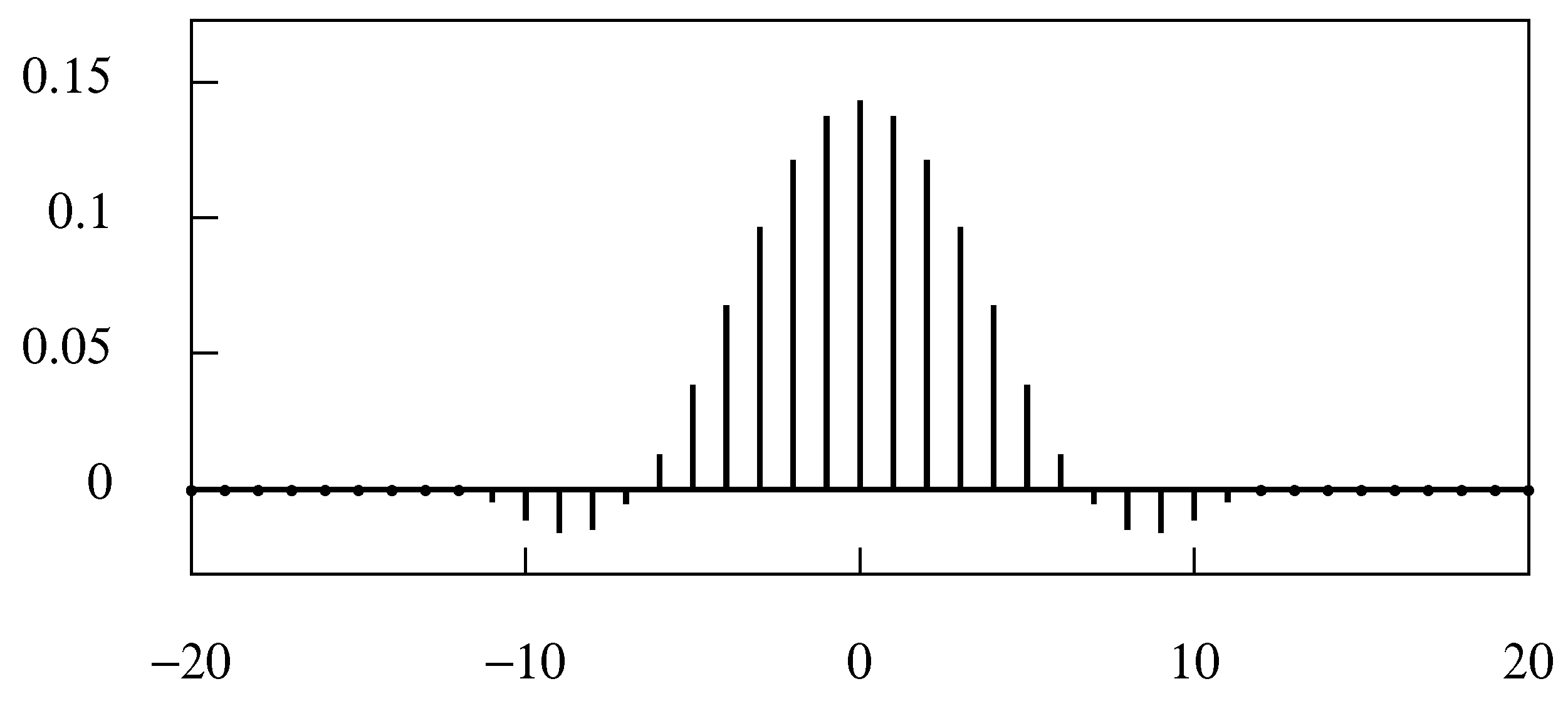
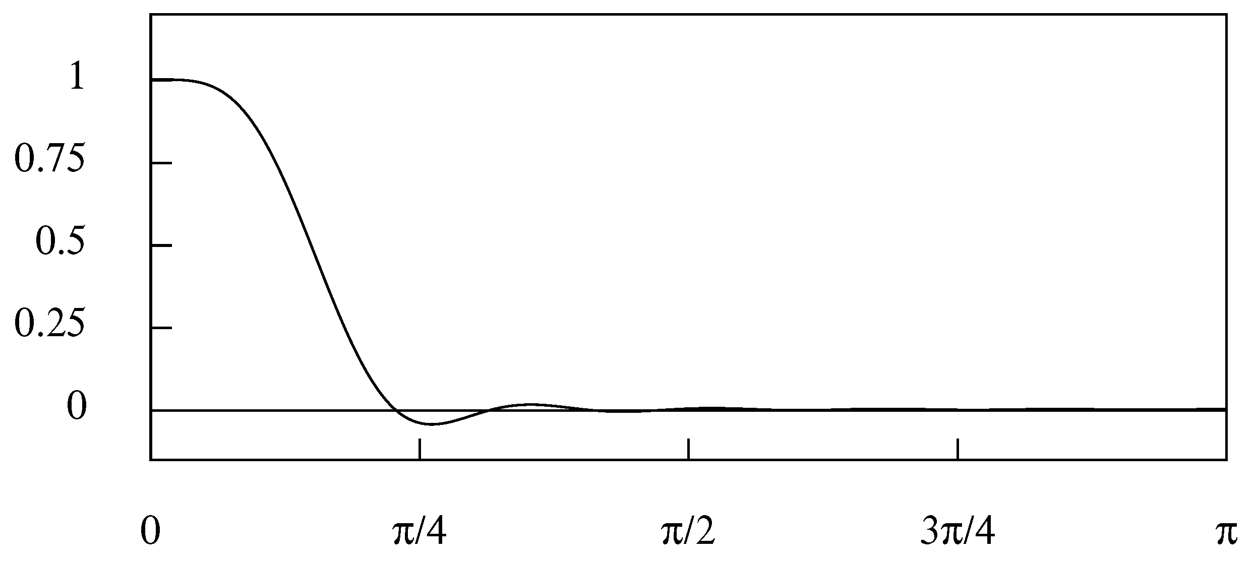
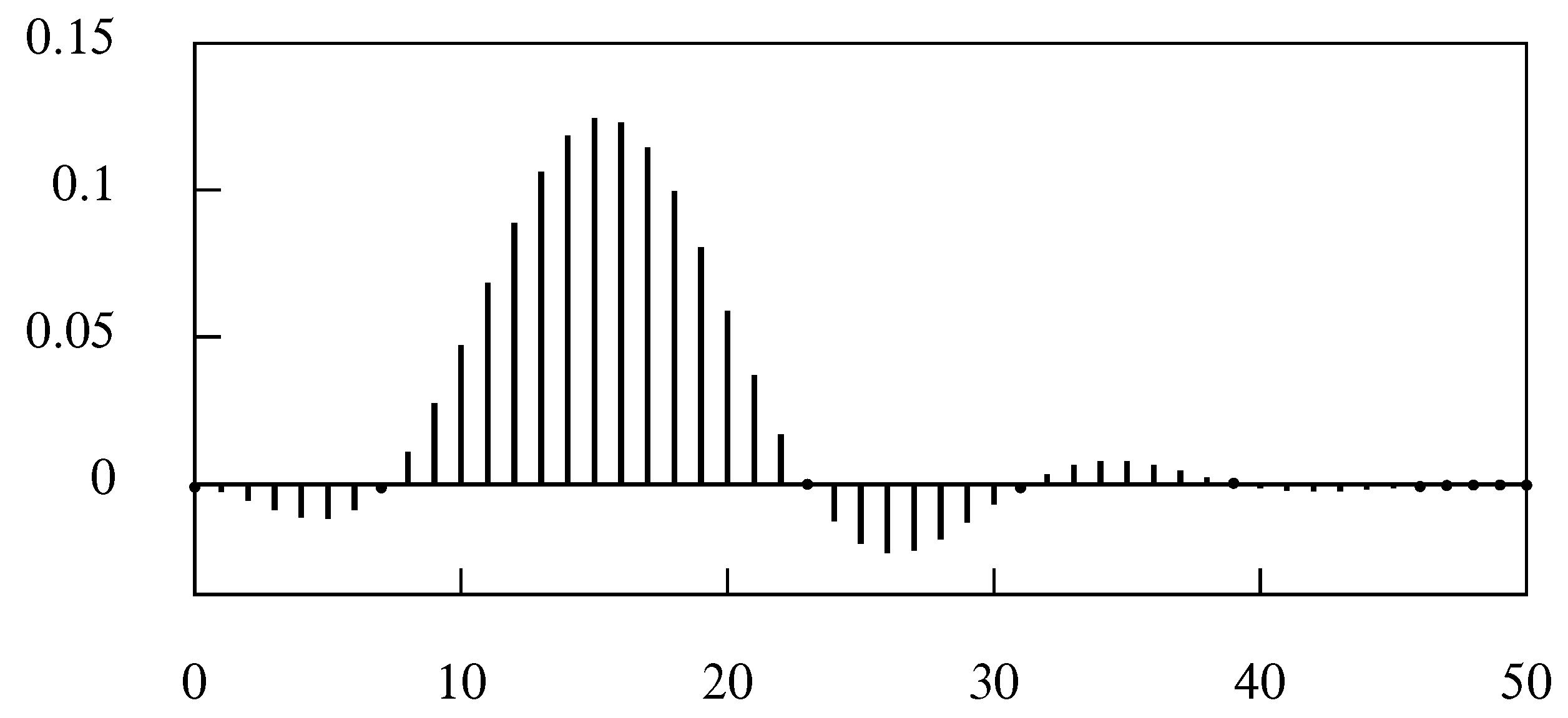
Figure 5 represents the coefficients of the symmetric Henderson moving-average filter of 23 points. Figure 6, which represents the frequency response function of the filter, shows a gradual transition from the pass band, which preserves the sinusoidal (or complex exponential) elements of a stationary process, to the stop band, which attenuates them and which ultimately nullifies them.

A symmetric moving-average filter that spans of $2m+1$ data points, and which looks equally forwards and backwards in time, encounters a problem when it reaches the ends of the data. Unless sets of m extra-sample points are added at both ends, the filter cannot process the first and the last m data points.

When the filter is applied to a mean-zero stationary process, it is reasonable to represent the extra-sample elements by their zero-valued expectations. This is not an appropriate recourse when the filter is applied directly to trended data with values that are remote from zero.

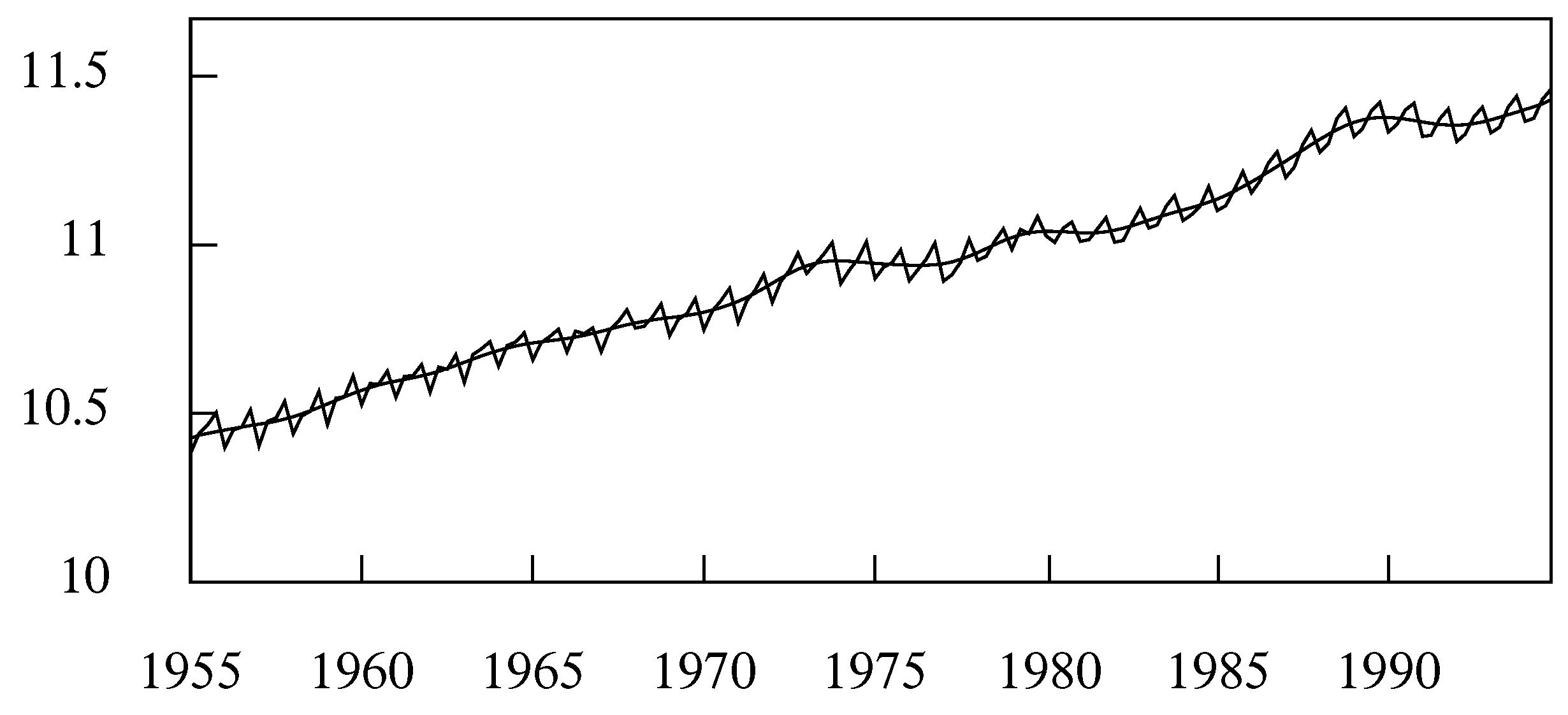
Since the Henderson filter is commonly applied directly to trended econometric data, such as are seen in Figure 7, it is necessary to deal effectively with the end-of-sample problem. Either the data must be extrapolated, or else the filter must be shortened so that it does not extend beyond the sample as it approaches the ends. In that case, the filter coefficients must be modified as the filter is collapsed.

As Wallis (1981) has shown, a procedure based on a time-invariant filter that overcomes the end-of-sample problem by using extrapolations based on sample values can be replaced by an equivalent procedure that applies a time-varying filter to points within the sample.

Various methods for extrapolating the sample and the equivalent means of modifying the filter coefficients have been proposed for the Henderson filters. Some of these have been cryptic and unexplained, as was the method proposed by Shiskin et al. (1967) for the filters within the X-11 program.

Since the Henderson filter is based on a cubic polynomial interpolation, it is natural to use a cubic function as the means of extrapolation. This approach has been adopted by Kenney and Durbin, who propounded an equivalent method for adapting the filter coefficients.

However, the method of adapting the coefficients that has been deployed in the X-11 program and its variants uses a linear extrapolation. The logic of that method has been uncovered by Doherty (2001), who has referenced the unpublished papers of Musgrave (1964a, 1964b) and of Laniel (1986) (see also Gray and Thomson (2002) for a discourse on the end-of-sample problem).

An alternative approach to constructing a filter is to define an appropriate frequency response and then to infer the coefficients of the corresponding filter to be applied in the time domain via a convolution with the data. However, it is also possible to conduct the filtering operation entirely in the frequency domain. This entails translating the data to the frequency domain and then translating them back to the time domain, once they have been processed.

In order to apply the frequency-domain methods, the data, which are treated as a circular sequence, must be devoid of trends. Therefore, methods are required for removing the trends from the data and for restoring the trends once the data have been filtered. Such methods will be described in Section 6. The need for complicated methods of data extrapolation that follow the trends in the data is alleviated in this approach.

4. The Ideal Filters

There may be a requirement for a more rapid transition from the pass band to the stop band of a filter than is available from the Henderson filter. Thus, for example, it has been the declared intention of Baxter and King (1999) to derive a filter that will isolate the components of an index of US GDP that have a cyclical duration of no less than six quarters (eighteen months) and of no more than 32 quarters (eight years). This prescription is due to a definition of the business cycle that was provided by Burns and Mitchell (1946).

Baxter and King sought to fulfill their requirement via a band pass filter that should, ideally, have instantaneous transitions at the two frequency values. In pursuit of such a filter, one may begin by defining an ideal low pass filter, which can be transformed to a band pass filter.

The ideal low pass filter with a positive-frequency cut-off point at ${\omega }_c$ is specified by the following periodic frequency response function, which has a period of $2\pi$ and which is specified over the interval $[-\pi ,\pi ]$ by

$$\lambda (\omega )=\left\{\begin{array}{cc}1,& \mathrm{if}\left|\omega \right|\in [0,{\omega }_c]);\hfill \\ 0,& \mathrm{otherwise}.\hfill \end{array}\right.$$

(19)

Within the interval $[0,\pi ]$, the sub interval $[0,{\omega }_c]$ is the pass band whilst the remainder $({\omega }_c,\pi ]$ is the stop band.

The coefficients of the low pass filter are given by the (inverse) Fourier transform of the periodic square wave:

$${\varphi }_j=\frac{1}{2\pi }{\int }_{-{\omega }_c}^{{\omega }_c}{e}^{\mathrm{i}\omega j}d\omega =\left\{\begin{array}{cc}{\displaystyle \frac{{\omega }_c}{\pi },}\hfill & \mathrm{if}j=0;\hfill \\ {\displaystyle \frac{sin({\omega }_{c}j)}{\pi j},}\hfill & \mathrm{if}j\ne 0.\hfill \end{array}\right.$$

(20)

The result for $j\ne 0$ follows by simple integration. The result for $j=0$ follows from setting $exp(\mathrm{i}\omega j)=exp(0)=1$ under the integral. Reference to Equation (9) shows that the coefficients are values sampled at unit intervals from the corresponding sinc function. This is illustrated in Figure 3 for the case where ${\omega }_c=\pi /2$. The resulting coefficients constitute a so-called ideal half-band filter.

4.1. Frequency Shifting

An ideal band pass filter with a positive-frequency pass band on the interval $[\alpha ,\beta ]$ is defined as follows:

$$\lambda (\omega )=\left\{\begin{array}{cc}1,\hfill & \mathrm{if}\left|\omega \right|\in [\alpha ,\beta ];\hfill \\ 0,\hfill & \mathrm{otherwise}.\hfill \end{array}\right.$$

(21)

The corresponding time-domain function is

$$\begin{array}{c}\hfill \begin{array}{ccc}{\displaystyle \varphi (t)=\frac{1}{2\pi }{\int }_{-\beta }^{-\alpha }{e}^{\mathrm{i}\omega t}d\omega +\frac{1}{2\pi }{\int }_{\alpha }^{\beta }{e}^{\mathrm{i}\omega t}d\omega }& =& {\displaystyle \left(\frac{e^{\mathrm{i}\beta t}-e^{-\mathrm{i}\beta t}}{2\pi \mathrm{i}t}\right)-\left(\frac{e^{\mathrm{i}\alpha t}-e^{-\mathrm{i}\alpha t}}{2\pi \mathrm{i}t}\right)}\hfill \\ & =& {\displaystyle \frac{1}{\pi t}\{sin(\beta t)-sin(\alpha t)\}.}\hfill \end{array}\end{array}$$

(22)

The identity $sin(A+B)-sin(A-B)=2cosAsinB$ can be used, with $\gamma =(\alpha +\beta )/2$ and $\delta =(\beta -\alpha )/2$, in place of A and B, to show that

$$\begin{array}{c}\hfill \begin{array}{ccc}{\displaystyle \varphi (t)=\frac{1}{\pi t}\{sin(\beta t)-sin(\alpha t)\}}& =& {\displaystyle \frac{2}{\pi t}cos\{(\alpha +\beta )t/2\}sin\{(\beta -\alpha )t/2\}}\hfill \\ & =& {\displaystyle \frac{2}{\pi t}cos(\gamma t)sin(\delta t).}\hfill \end{array}\end{array}$$

(23)

The centre of the pass band is $\gamma$, whereas $\delta$ is half its width. The cut-off points of the pass band are $\alpha ,\beta \in [0,\pi ]$. The low pass prototype filter is $sin(\delta t)/(\pi t)$, whereas $2cos(\gamma t)$ affects the frequency shifting.

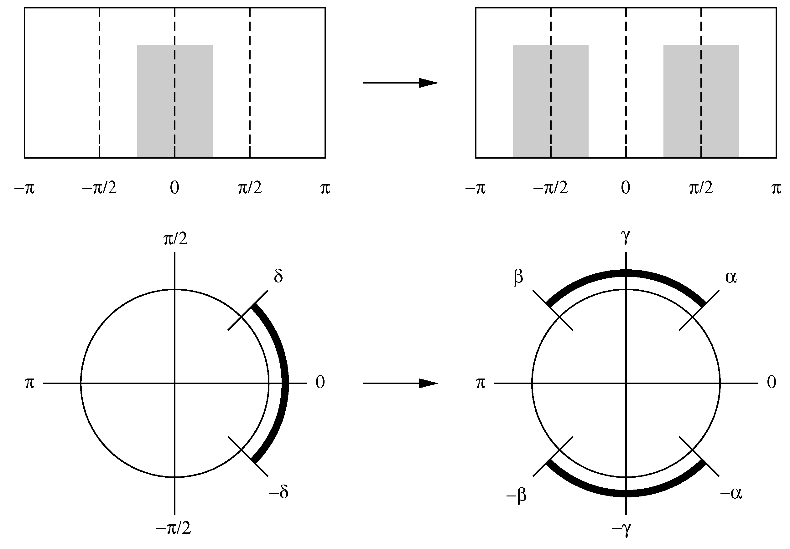
This effect of frequency shifting can be understood by recognising that $2cos(\gamma t)\zeta (t)=e^{\mathrm{i}\gamma t}\zeta (t)+e^{-\mathrm{i}\gamma t}\zeta (t)$. Thus, in Equation (23), two copies are made of the function $\zeta (t)=sin(\delta t)/\pi t$, which has a pass band on the interval $[-\delta ,\delta ]$, and these are shifted so that their centres lie at $-\gamma$ and $\gamma$. Then, $\gamma \pm \delta =\alpha ,\beta$ and $-\gamma \pm \delta =-\beta ,-\alpha$. Figure 8 provides two representations of a frequency shift.

4.2. Truncating the Filter

A difficulty in applying the ideal filters that have been specified above lies in the fact that they entail an infinite number of coefficients. One way of addressing the problem is to truncate the filters by taking only a limited number of central coefficients to create what is described as a finite impulse-response (FIR) filter.

The coefficients of a band pass or a high pass filter must sum to zero, whereas the coefficients of a low pass filter must sum to unity. The coefficients of a truncated filter must be rescaled so as to meet these requirements. Constraining the coefficients to sum to zero ensures the the z-transform polynomial has a root of unity, such the $\varphi (1)={\sum }_j{\varphi }_j=0$. This implies that $\nabla (z)=1-z$ is a factor of the polynomial, which indicates that the filter incorporates a difference operator.

If the filter is symmetric, such that $\psi (z)={\psi }_0+{\psi }_1(z+z^{-1})+\cdots +{\psi }_m(z^m+z^{-m})$ and, therefore, $\psi (z)=\psi (z^{-1})$, then $1-z^{-1}$ is also a factor. Therefore, $\psi (z)$ has the combined factor $(1-z)(1-z^{-1})=-z^{-1}{\nabla }^2(z)$, which indicates that the filter incorporates a twofold differencing operator. Such a filter is effective in reducing a linear trend to zero; and, therefore, it is applicable to the logarithms of econometric data sequences that have an underlying log-linear or exponential trend.

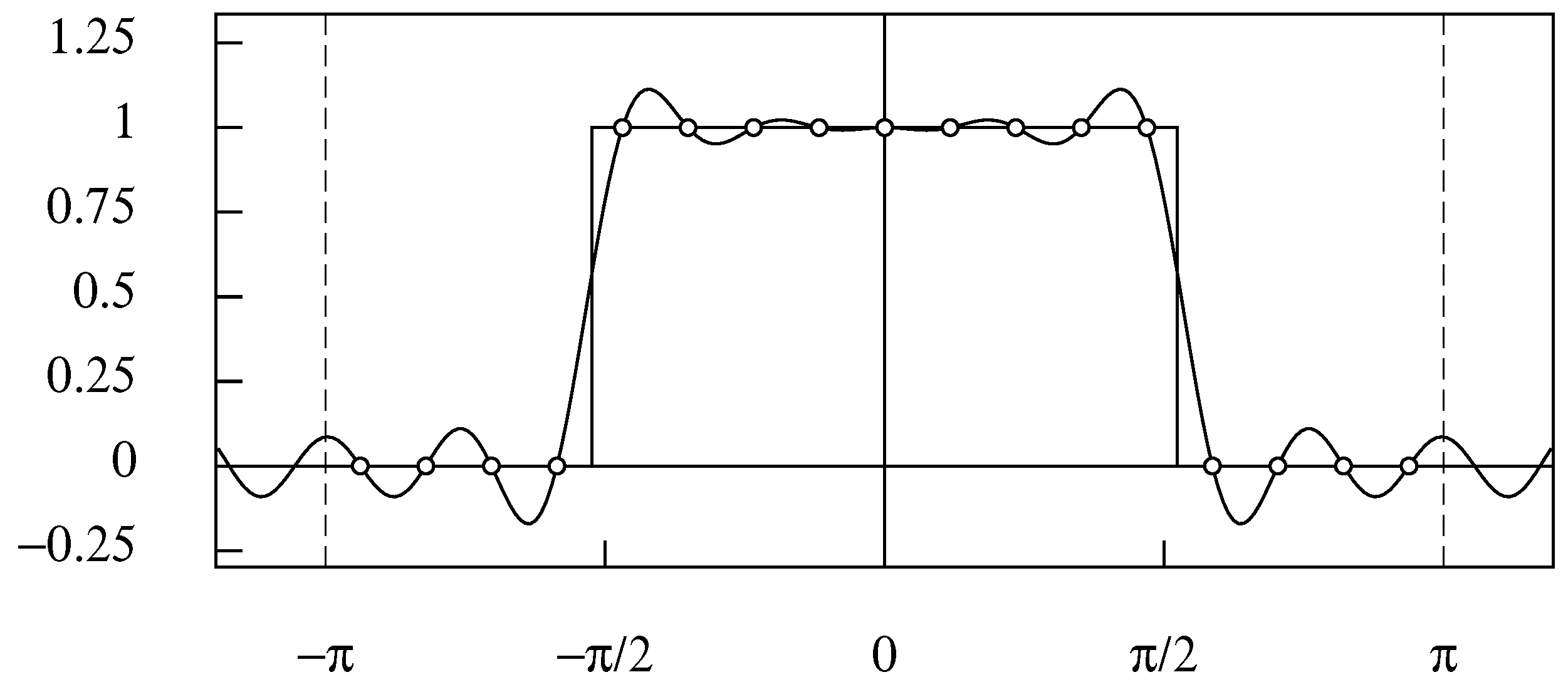
The effect of truncating the filter will be to create a frequency response that departs from the ideal square-wave response and that may allow a substantial leakage to occur in the stop band, whereby elements of the data are transmitted that should be blocked (see Figure 9).

A further problem with such filters is that they cannot reach the ends of a data sample. Thus, a symmetric filter of $2m+1$ coefficients will be unable to process the first and the last m data values unless the sample is extrapolated. The matter has been raised in Section 3, but a full consideration of the problem will be deferred until Section 6.

4.3. The Ideal Filters in the Frequency Domain

One way of overcoming the problems of leakage is to work with the discrete Fourier transform of the finite data sequence $\{x_t;t=0,1,\dots ,T-1\}$, which gives rise to the sequence $\{{\xi }_j;j=0,1,\dots ,T-1\}$ of Fourier ordinates:

$$x_t=\sum _{j=0}^{T-1}{\xi }_j{e}^{\mathrm{i}{\omega }_{j}t}⟷{\xi }_j=\frac{1}{T}\sum _{t=0}^{T-1}{x}_t{e}^{-\mathrm{i}{\omega }_{j}t},\mathrm{where}{\omega }_j=\frac{2\pi }{T}.$$

(24)

In this context, both the data sequence and the sequence of Fourier ordinates are to be regarded as circular or periodic functions, with the former supported on the interval $[0,T)$ and the latter on the interval $[0,2\pi )$.

An ideal filter can be applied to a finite sample by operating on the ordinates ${\xi }_j$ of its Fourier transform. The ordinates that fall within the pass band are preserved while those that fall within the stop band are replaced by zeros. Then, the preserved ordinates are translated back into the time domain by the inverse transform.

An alternative and a less adept way of applying an ideal filter is to generate the time-domain coefficients of a circular filter that can be convoluted with the circularised data.

Consider a set of T frequency-domain ordinates sampled from a periodic square-wave or boxcar function, centred on ${\omega }_0=0$, at the Fourier frequencies ${\omega }_j=2\pi j/T;j=0,\pm 1,\dots ,\pm [T/2]$ that fall within the interval $[-\pi ,\pi ]$. (For convenience, the frequency interval $[0,2\pi ]$ of the discrete Fourier transform can be replaced by the interval $[-\pi ,\pi ]$ without affecting the analysis). If the cut-off points are at $\pm {\omega }_d=\pm d{\omega }_1=\pm 2\pi d/T$, then the ordinates of the sample will be

$${\lambda }_j=\left\{\begin{array}{cc}1,& \mathrm{if}j\in \{1-d,\dots ,d-1\},\hfill \\ 1/2,& \mathrm{if}j=\pm d,\hfill \\ 0,& \mathrm{otherwise}.\hfill \end{array}\right.$$

(25)

Since this is to be construed as a periodic function of period T, it follows that ${\lambda }_{-j}={\lambda }_{T-j}$, which allows the (discrete) Fourier transform of the circular filter coefficients to be expressed as

$${\varphi }_k^{\circ }=\sum _{j=0}^{T-1}{\lambda }_j{e}^{\mathrm{i}{\omega }_{j}k}⟷{\lambda }_j=\frac{1}{T}\sum _{k=0}^{T-1}{\varphi }_k^{\circ }{e}^{-\mathrm{i}{\omega }_{j}k}.$$

(26)

This may be compared with the discrete-time Fourier transform that generates a doubly-infinite sequence of filter coefficients:

$${\varphi }_k=\frac{1}{2\pi }{\int }_{-\pi }^{\pi }\lambda (\omega )e^{\mathrm{i}\omega k}d\omega ⟷\lambda (\omega )=\sum _{k=-\infty }^{\infty }{\varphi }_k{e}^{-\mathrm{i}\omega k}.$$

(27)

Since ${\lambda }_j=\lambda ({\omega }_j)$ at the point ${\omega }_j=2\pi j/T$, it follows, on comparing the RHS of (27) with that of (26), that

$$\frac{1}{T}{\varphi }_k^{\circ }=\sum _{q=-\infty }^{\infty }{\varphi }_{k+qT}\mathrm{for}k=0,1,\dots ,T-1.$$

(28)

Thus, the circular coefficients $\{{\varphi }_k^{\circ };k=0,1,\dots ,T-1\}$ would result from wrapping the infinite coefficient sequence $\{{\varphi }_k;k=0,\pm 1,\pm 2,\dots \}$ around a circle of circumference T and adding the overlying ordinates.

This is impractical and, therefore, the circulant filter coefficients would be created, in practice, by applying a discrete Fourier transform to the corresponding frequency-domain ordinates $\{{\lambda }_j\}$ to carry them into the time domain.

The formula for the wrapped circulant filter that fulfills the specification of (25) is

$${\varphi }^{\circ }(k)=\left\{\begin{array}{cc}{\displaystyle \frac{2d}{T},}& \mathrm{if}k=0,\hfill \\ {\displaystyle \frac{cos({\omega }_{1}k/2)sin(d{\omega }_{1}k)}{Tsin({\omega }_{1}k/2)},}& \mathrm{for}k=1,\dots ,T-1,\hfill \end{array}\right.$$

(29)

where ${\omega }_1=2\pi /T$.

In an alternative specification of the ideal filter, the cut-off points fall between Fourier frequencies. Then, the ordinates sampled from the frequency response function are

$${\lambda }_j=\left\{\begin{array}{cc}1,& \mathrm{if}j\in \{1-d,\dots ,d-1\},\hfill \\ 0,& \mathrm{otherwise},\hfill \end{array}\right.$$

(30)

and the formula of the filter coefficients is

$${\varphi }^{\circ }(k)=\left\{\begin{array}{cc}{\displaystyle \frac{2(d-1)}{T},}& \mathrm{if}k=0,\hfill \\ {\displaystyle \frac{sin([d-1/2]{\omega }_{1}k)}{Tsin({\omega }_{1}k/2)}}& \mathrm{for}k=1,\dots ,T-1.\hfill \end{array}\right.$$

(31)

The coefficients of the Dirichlet kernels can be disposed symmetrically about the midpoint of the sequence of $k=0,1,\dots ,T-1$. The formulae of (29) and (31), which are (A25) and (A28) in the appendix A.3, are also to be found in an appendix to Pollock (2008).

4.4. The Band pass Specification

One might wish to construct a wrapped filter according to the more general band pass specification:

$$\varphi (\omega )=\left\{\begin{array}{cc}1,& \mathrm{if}\left|\omega \right|\in ({\omega }_a,{\omega }_b),\hfill \\ 1/2,& \mathrm{if}\omega =\pm {\omega }_a,\pm {\omega }_b,\hfill \\ 0,& \mathrm{for}\omega \mathrm{elsewhere}\mathrm{in}[-\pi ,\pi ),\hfill \end{array}\right.$$

(32)

where ${\omega }_a=a{\omega }_1$ and ${\omega }_b=b{\omega }_1$, and where it is assumed that T is even. For the ideal filter, this can be achieved by subtracting one filter from another to create

$$\begin{array}{ccc}\hfill {\varphi }_{[a,b]}^{\circ }(k)& =& {\varphi }_b^{\circ }(k)-{\varphi }_a^{\circ }(k)\hfill \\ & =& \frac{cos({\omega }_{1}k/2)\{sin(b{\omega }_{1}k)-sin(a{\omega }_{1}k)\}}{Tsin({\omega }_{1}k/2)}\hfill \\ & =& 2cos(g{\omega }_{1}k)\frac{cos({\omega }_{1}k/2)sin(d{\omega }_{1}k)}{Tsin({\omega }_{1}k/2)}.\hfill \end{array}$$

(33)

Here, $2d=b-a$ is the width of the pass band (measured in terms of a number of sampled points) and $g=(a+b)/2$ is the index of its centre. The final expression follows from the identity $sin(A+B)-sin(A-B)=2cosAsinB$. The expression can be interpreted as the result of shifting a low pass filter with a cut-off frequency at the point d so that its centre is moved from 0 to the point g. The technique of frequency shifting is not confined to the ideal frequency response. It can be applied to any frequency response function.

There is a prevalent notion that an ideal filter cannot be realised in practice, for the reason that to achieve an instant transition in the frequency response from a pass band to a stop band requires an infinite number of filter coefficients.

Although the frequency response ${\lambda }_j=\lambda ({\omega }_j)$ of the finite-sample filter is defined only for T frequency points, it can be insightful to consider the function $\lambda (\omega )={\sum }_k{\varphi }_k^{\circ }exp(-\mathrm{i}\omega )$, where $\omega$ varies continuously in the interval $[-\pi ,\pi ).$ Then, there is no requirement that the frequency response of the ideal filter should make an instant transition.

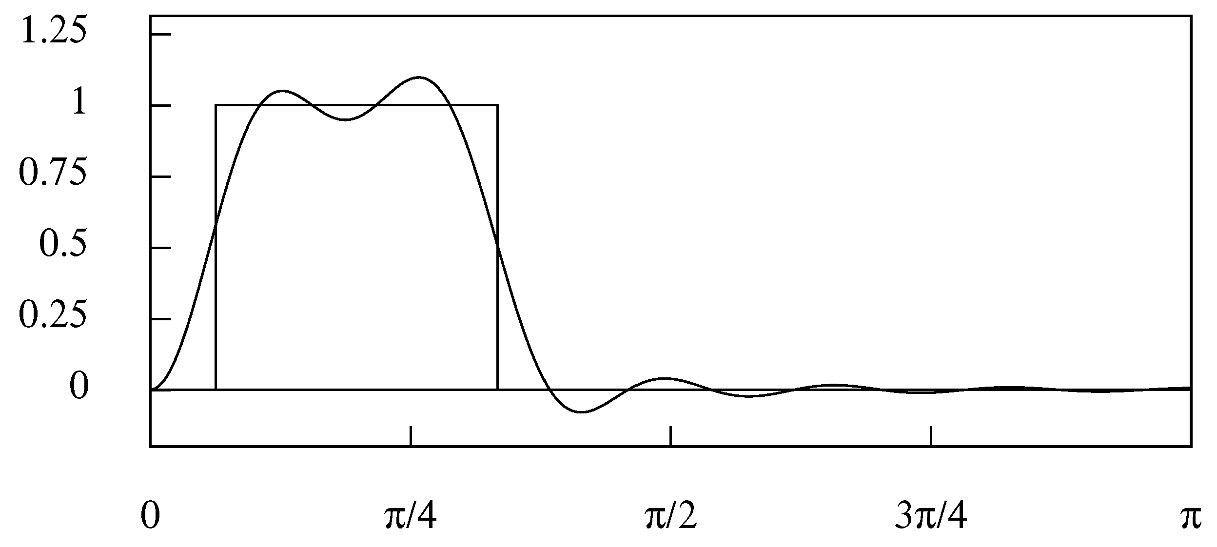
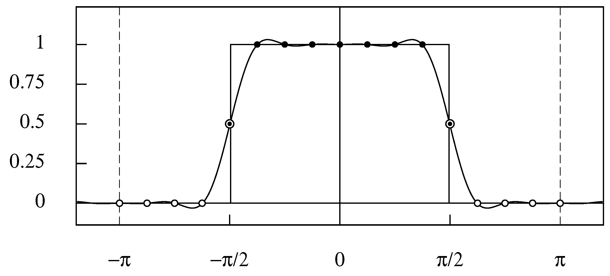
The matter can be elucidated by considering low pass half-band filter with a cut-off frequency of $\pi /2$. In the case of an even sample size, where the midpoint of the transition is at the nominal cut-off point, the transitions occur within the interstices between that point and the adjacent frequency points on either side (see Figure 10). In the case of an odd sample size, the transition occurs between two adjacent frequency points (see Figure 11).

4.5. Interpolating a Finite Data Sequence

Dirichlet kernels provide a way of interpolating a finite data sequence. Consider again the discrete Fourier transform expressed as follows:

$$x_t=\sum _{j=0}^{T-1}{\xi }_j{e}^{\mathrm{i}{\omega }_{j}t}⟷{\xi }_j=\frac{1}{T}\sum _{t=0}^{T-1}{x}_t{e}^{-\mathrm{i}{\omega }_{j}t}\mathrm{with}{\omega }_j=\frac{2\pi j}{T}.$$

(34)

By putting the RHS of the latter into the LHS and commuting the two summations and allowing $t\in [0,T)$ to vary continuously, and assuming that T is odd, we get

$$x(t)=\frac{1}{T}\sum _{k=0}^{T-1}{x}_k\left\{\sum _{j=0}^{T-1}{e}^{\mathrm{i}{\omega }_j(t-k)}\right\}=\frac{1}{T}\sum _{k=0}^{T-1}{x}_k{\phi }^{\circ }(t-k),$$

(35)

When T is odd, there is

$$\frac{1}{T}{\phi }^{\circ }(t)=\sum _{j=0}^{T-1}{e}^{\mathrm{i}{\omega }_{j}t}=\frac{sin(n{\omega }_{1}t)}{Tsin({\omega }_{1}t/2)}\mathrm{with}n=\frac{T-1}{2},$$

(36)

which is the periodic Dirichlet Kernel supported on the Nyquist interval. When T is even, $\phi (t)/T$ is provided by the formula of (29) with $d=T/2$.

Equations (34) and (35) imply that a sinc function interpolation of a finite data sequence that employs a sequence of Dirichlet kernels is equivalent to an interpolation based on a Fourier synthesis. Thus, a simpler way of recovering a continuous trajectory from the sampled sequence is to allow the index t to vary continuously in the interval $[0,T)$ within the expression for the sequence that is provided by the discrete Fourier transform. The resulting trajectory is

$$x(t)=\sum _{j=0}^{[T/2]}\left\{{\alpha }_{j}cos({\omega }_{j}t)+{\beta }_{j}sin({\omega }_{j}t)\right\}=\sum _{j=0}^{T-1}{\xi }_j{e}^{\mathrm{i}{\omega }_{j}t},$$

(37)

where ${\omega }_j=2\pi j/T;j=0,1,\dots ,[T/2]$ are the Fourier frequencies, which are placed at regular intervals running from zero to the Nyquist frequency of $\pi$. Here, $[T/2]$ denotes the integer quotient of the division of T by 2.

The trigonometric functions and the complex exponential functions of (37) are connected via Euler’s equations (A1) and (A2) of Appendix A.1. In addition, ${\xi }_j={\alpha }_j-\mathrm{i}{\beta }_j$ and ${\xi }_{T-j}={\alpha }_j+\mathrm{i}{\beta }_j$ for $j=0,1,\dots ,[T/2]$. The coefficients ${\alpha }_j,{\beta }_j$ are obtained by regressing the data on the ordinates of the trigonometric functions $cos({\omega }_{j}t),sin({\omega }_{j}t)$, where $t=0,1,\dots ,T-1$.

4.6. Resampling the Data

A Fourier interpolation, or the equivalent Dirichlet-kernel interpolation, can be employed whenever it is appropriate to lower the rate of the sampling of a data sequence.

The periodogram of the sequence may reveal that the continuous process from which the sampled data are derived has a frequency limit, expressed in terms of radians per sampling interval, of ${\omega }_c<\pi$, which is below the Nyquist limit. This will be an impediment to fitting a linear time-series model, which presupposes that the spectrum of the sampled process is supported on the interval $[0,\pi ]$.

To ensure that the maximum frequency of the data coincides with the Nyquist frequency of $\pi$ radians per (unit) sample interval, one can regenerate the continuous trajectory by a Fourier synthesis. Thereafter, the interpolated trajectory can be resampled at the wider intervals of $\pi /{\omega }_c$ time units.

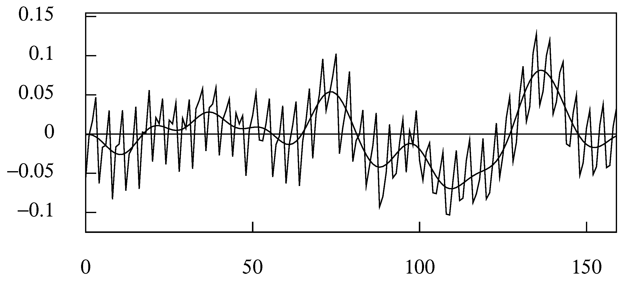
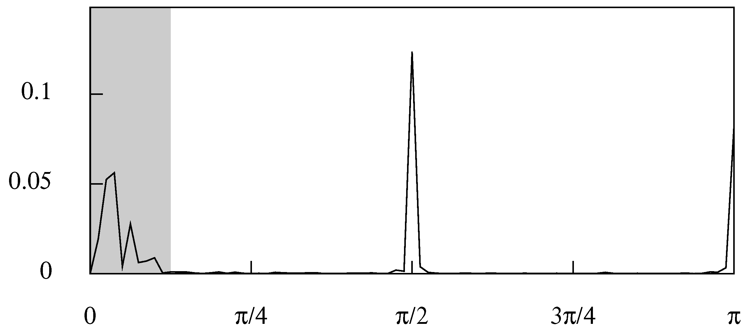
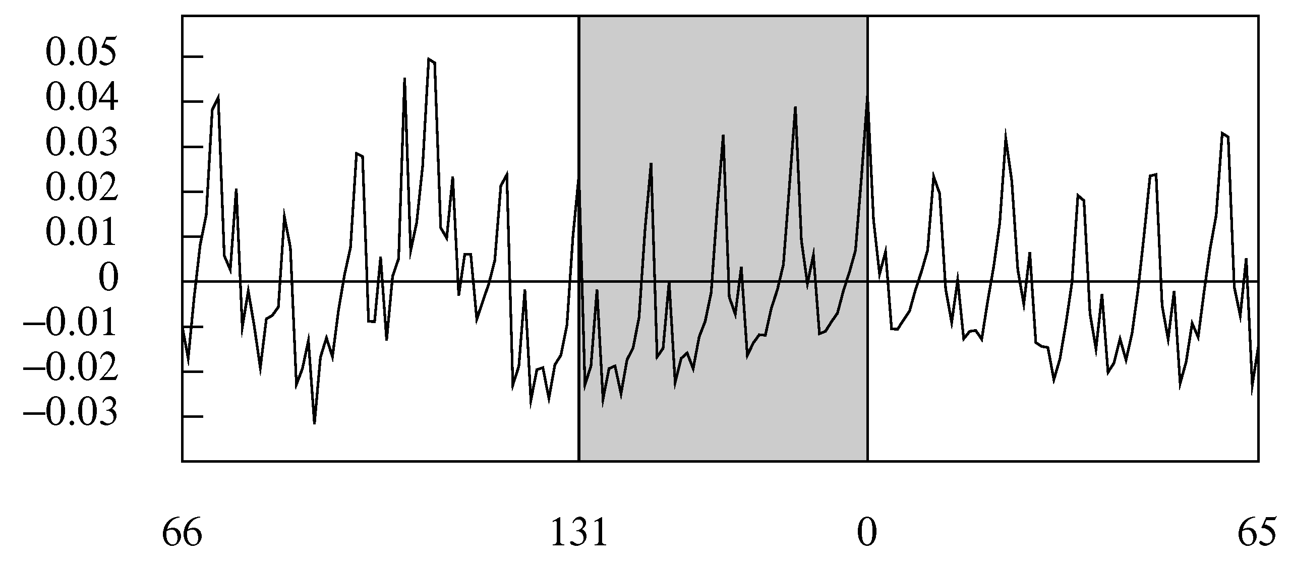
Figure 12 shows the deviations from a linear trend of the logarithms of a quarterly sequence of U.K. domestic expenditure. The data are beset by seasonal fluctuations that have a frequency of $\pi /2$ radians per sampling interval. However, Figure 13 shows that the business cycle, which accounts for the major fluctuations, has a spectra structure that falls within a shaded band bounded by a maximum frequency of ${\omega }_c=\pi /8$ radians per sampling interval.

A smooth trajectory, corresponding to the business cycle, can be synthsised from the Fourier coefficients that fall in the interval $[0,\pi /8]$. The trajectory, which can be envisaged as a product of an ideal low pass filtering operation, is depicted in Figure 12. The sample on which the ARMA model should be based could be obtained by resampling this trajectory at the rate of one observation in every $\pi /{\omega }_c$ time units.

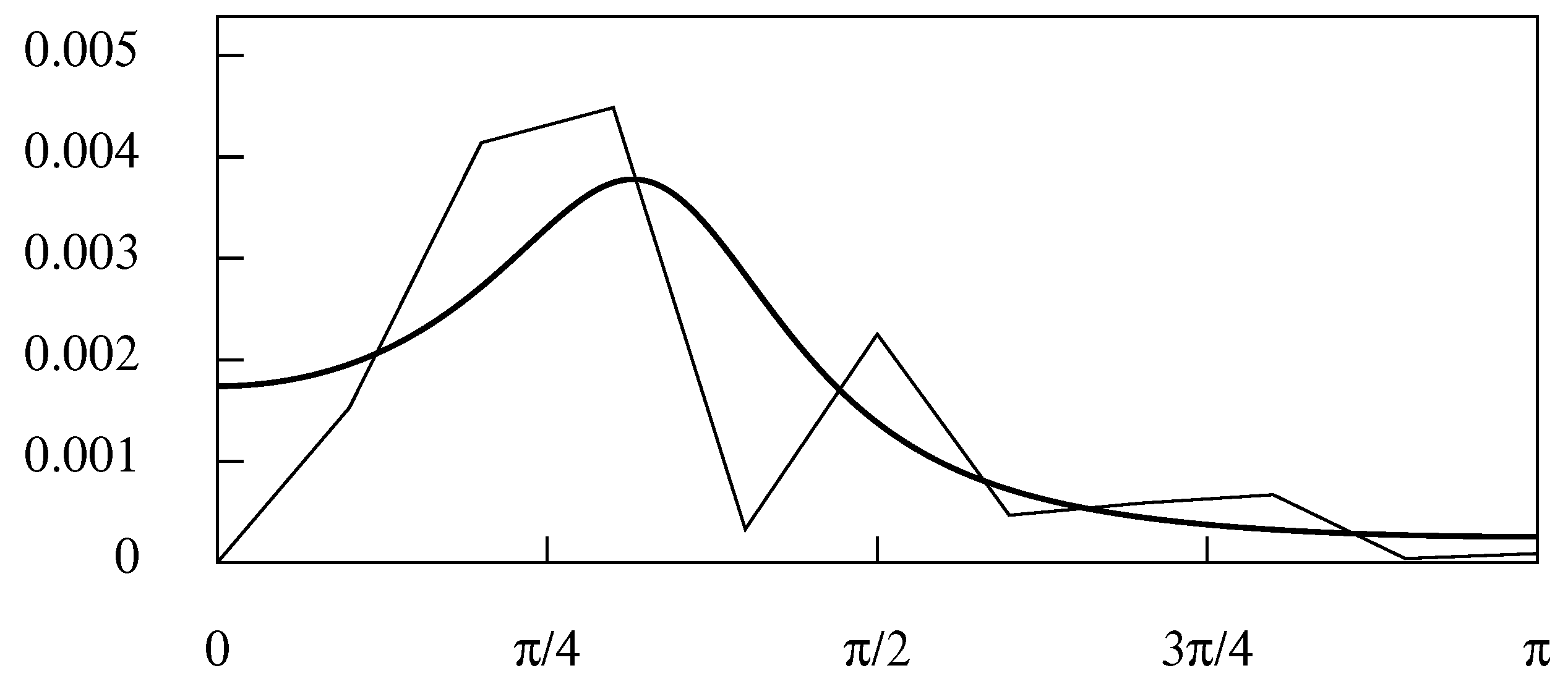
However, in this case, it is sufficient to obtain the sample by taking one in every eight of the data points of the filtered sequence. The periodogram of the subsampled data, overlayed by the parametric spectrum of an estimated second-order autoregressive model, is shown in Figure 14. This periodogram is an expanded version of the spectral structure that is highlighted in Figure 13.

5. Graded Filters

An instantaneous event will be represented in a continuous-time data steam by an isolated spike. The spectral signature of such an impulse is spread uniformly over the entire real line. An instantaneous event will also be reflected in a sampled data sequence by a discrete impulse, which has a uniform spectrum over the interval $[-\pi ,\pi ]$.

The effect of filtering the sequence by an ideal low pass filter will be to remove the high-frequency component of the impulse. This is liable to make the event undetectable in the smoothed sequence, which will lack the necessary temporal resolution.

According to Heisenberg’s uncertainty principle, there is an inverse relationship between the dispersion of a function in the time domain and the dispersion of its Fourier transform in the frequency domain. Therefore, in order to improve the temporal resolution of the smoothed sequence, one should increase the dispersion of the frequency response function of the filter. This can be achieved by allowing a gradual transition from the pass band to the stop band.

5.1. Gaussian Filters

Heisenberg’s uncertainty principle places a bound on the product of the dispersion of a function and that of its Fourier transform. The bound is attained by the Gaussian function and its transform, which is also a Gaussian function. By adopting this function, one can achieve an optimum trade-off of the resolutions of the two domains. (For an excellent brief account of the uncertainty principle, in which there is also a characterisation of the sinc function, see Nahin 2006).

The Gaussian function and its Fourier transform are given by

$$f(t)=\frac{1}{\sqrt{2\pi {\sigma }_t^2}}exp\left\{-\frac{t^2}{2{\sigma }_t^2}\right\}⟷\varphi (\omega )=exp\left\{-\frac{{\omega }^2}{2{\sigma }_{\omega }^2}\right\},$$

(38)

where ${\sigma }_t\times {\sigma }_{\omega }=1/(2\pi )$, which is the product of the standard deviations.

The function is continuous and, in common with its transform, it is supported on the entire real line. Therefore, in order to create a viable discrete-time filter, it is necessary to sample the function and to truncate the resulting sequence. Since the function decays rapidly, it may be acceptable to form a time-domain filter from a limited number of the sampled coefficients, indexed by $t=0,\pm 1,\pm 2,\dots ,\pm m$, where $m=C{\sigma }_t+1$, with $C\in [3,\dots ,6]$.

A two-dimensional Gaussian filter is commonly used in image processing. The one-dimensional filter can be used in a time-series analysis when it is required to smooth a data sequence of which the spectrum extends over the Nyquist range and when there are no clearly delimited spectral structures that one might wish to isolate.

5.2. The Binomial Filter

An alternative way of creating a graded low pass filter is to employ the approximations to a Gaussian distribution that are provided by the binomial distribution. The $n+1$ coefficients of the low pass filter are

$$b(x;n,p,q)=\frac{n!}{x!(n-x)!}{p}^x{q}^{n-x}\mathrm{with}p=q=\frac{1}{2},$$

(39)

where $x=0,1,\dots ,n$. The coefficients of the filter can be generated via a simple recursion that connects

$$b_j=\frac{n!}{j!(n-j)!}{p}^j{q}^{n-j}\mathrm{and}{b}_{j-1}=\frac{n!}{(j-1)!(n-j+1)!}{p}^{j+1}{q}^{n-j-1}.$$

(40)

When $p=q=1/2$, the ratio of the two is $b_j/b_{j-1}=(n-j+1)/j$, whence

$$b_j=\frac{n-j+1}{j}{b}_{j-1}\mathrm{with}{b}_0=p^n={0.5}^n.$$

(41)

The z-transform of the sequence of binomial coefficients is ${(1+z)}^n/2^n$. This corresponds to a one-sided filter that looks only backward in time. The z-transform of the symmetric phase-neutral binomial filter is

$$b(z)=\frac{{(1+z^{-1})}^m{(1+z)}^m}{2^n}\mathrm{where}m=\frac{n}{2},$$

(42)

which is obtained by multiplying that of the backward-looking filter by $z^{-m}$ to shift it forwards in time. The frequency response, which is obtained by setting $z=exp\{-\mathrm{i}\omega \}$ and by invoking the result (A8) of the appendix, is

$$b_n(\omega )={\{cos(\omega /2)\}}^n.$$

(43)

In common with other FIR filters, the binomial filter cannot reach the ends of the sample unless the data are supplemented at both ends by m extra-sample points. We continue to assume that the data are free of trends. In that case, the extra points can be provided by reflecting the succeeding and preceding m points around the lower and the upper end points respectively and thereafter, if necessary, by applying a taper that successively reduces the absolute values of these points as their distances from the end points increase (see Section 6.1).

5.3. Wiener–Kolmogorov Filters and the Butterworth Filter

In practice, one might wish to choose the cut-off frequency for the filter and to proceed to determine an appropriate rate of transition about that point. The Butterworth filter is appropriate to this purpose.

The complementary low pass and high pass Butterworth filters, denoted by ${\psi }_L(z)$ and ${\psi }_H(z)$, respectively, fulfil the following conditions:

$$\begin{array}{cc}\hfill (\mathrm{i})& {\psi }_L(z)+{\psi }_H(z)=1\mathit{Complementarity},\hfill \\ \hfill (\mathrm{ii})& {\psi }_L(z^{-1})={\psi }_L(z),{\psi }_H(z^{-1})={\psi }_H(z)\mathit{Phase-Neutrality},\hfill \\ \hfill (\mathrm{iii})& |{\psi }_L(1)|=1,|{\psi }_L(-1)|=0\mathit{Low}\mathit{Pass}\mathit{Conditions},\hfill \\ \hfill (\mathrm{iv})& |{\psi }_H(1)|=0,|{\psi }_H(-1)|=1.\mathit{High}\mathit{Pass}\mathit{Conditions}.\hfill \end{array}$$

(44)

The conditions of phase neutrality of (ii) are by virtue of the symmetry of the filters. The conditions of complementarity and phase neutrality under (i) and (ii) are satisfied by specifying that

$${\psi }_L(z)=\frac{{\delta }_L(z^{-1}){\delta }_L(z)}{\gamma (z^{-1})\gamma (z)}\mathrm{and}{\psi }_H(z)=\frac{{\delta }_H(z^{-1}){\delta }_H(z)}{\gamma (z^{-1})\gamma (z)},$$

(45)

where

$$\gamma (z^{-1})\gamma (z)={\delta }_L(z^{-1}){\delta }_L(z)+{\delta }_H(z^{-1}){\delta }_H(z).$$

(46)

These two equations define the structure of a Wiener–Kolmogorov digital filter.

The condition under (iii) and (iv) ensure that the low pass filter has unit gain at zero frequency and that the high pass filter has unit gain at the Nyquist frequency of $\pi$. They can be satisfied by specifying that

$${\delta }_L(z)={\lambda }_L{(1+z)}^n\mathrm{and}{\delta }_H(z)={\lambda }_H{(1-z)}^n,$$

(47)

where n is a positive integer. Putting these specifications into (45) and (46) gives

$$\begin{array}{ccc}{\psi }_L(z)& =& {\displaystyle \frac{{(1+z^{-1})}^n{(1+z)}^n}{{(1+z^{-1})}^n{(1+z)}^n+\lambda {(1-z^{-1})}^n{(1-z)}^n}}\hfill \\ & =& {\displaystyle \frac{1}{1+\lambda {\left({\displaystyle \mathrm{i}\frac{1-z}{1+z}}\right)}^{2n}},\mathrm{where}\lambda =\frac{{\lambda }_H^2}{{\lambda }_L^2}}\hfill \end{array}$$

(48)

and

$$\begin{array}{c}\hfill \begin{array}{ccc}{\psi }_H(z)& =& {\displaystyle \frac{{(1-z^{-1})}^n{(1-z)}^n}{{\lambda }^{-1}{(1+z^{-1})}^n{(1+z)}^n+{(1-z^{-1})}^n{(1-z)}^n}}\hfill \\ & =& {\displaystyle \frac{1}{1+{\lambda }^{-1}{\left({\displaystyle \mathrm{i}\frac{1+z}{1-z}}\right)}^{2n}}.}\hfill \end{array}\end{array}$$

(49)

When $z=exp\{\mathrm{i}\omega \}$ within

$$\mathrm{i}\frac{1-z}{1+z}=\mathrm{i}\frac{z^{-1/2}-z^{1/2}}{z^{-1/2}+z^{1/2}},$$

(50)

this becomes the ratio of $sin(\omega /2)$ and $cos(\omega /2)$, which is $tan(\omega /2)$. It follows that the frequency response functions of the low pass and high pass filters are

$${\psi }_L(\omega )=\frac{1}{1+\lambda {\{tan(\omega /2)\}}^{2n}}\mathrm{and}{\psi }_H(\omega )=\frac{1}{1+{\lambda }^{-1}{\{\mathrm{cotan}(\omega /2)\}}^{2n}}.$$

(51)

The parameter $\lambda$ governs the location of the midpoint of the transition from the pass band to the stop band of the low pass filter and conversely for the high pass filter. It will be observed that, when $\lambda =1$, there is a perfect symmetry between the two filters, which become the reflections of each other about a vertical line located at the frequency value of $\pi /2$. Moreover, at that point, which is the midpoint of both transitions, the value of the gain is $1/2$.

The midpoint of the transition can be located at any frequency ${\omega }_c\in (0,\pi )$. By solving the equation ${\psi }_L({\omega }_c)=1/2$, it is found that the value of $\lambda$ that locates the midpoint at ${\omega }_c$ is

$$\lambda ={\{\mathrm{cotan}({\omega }_c/2)\}}^{2n}.$$

(52)

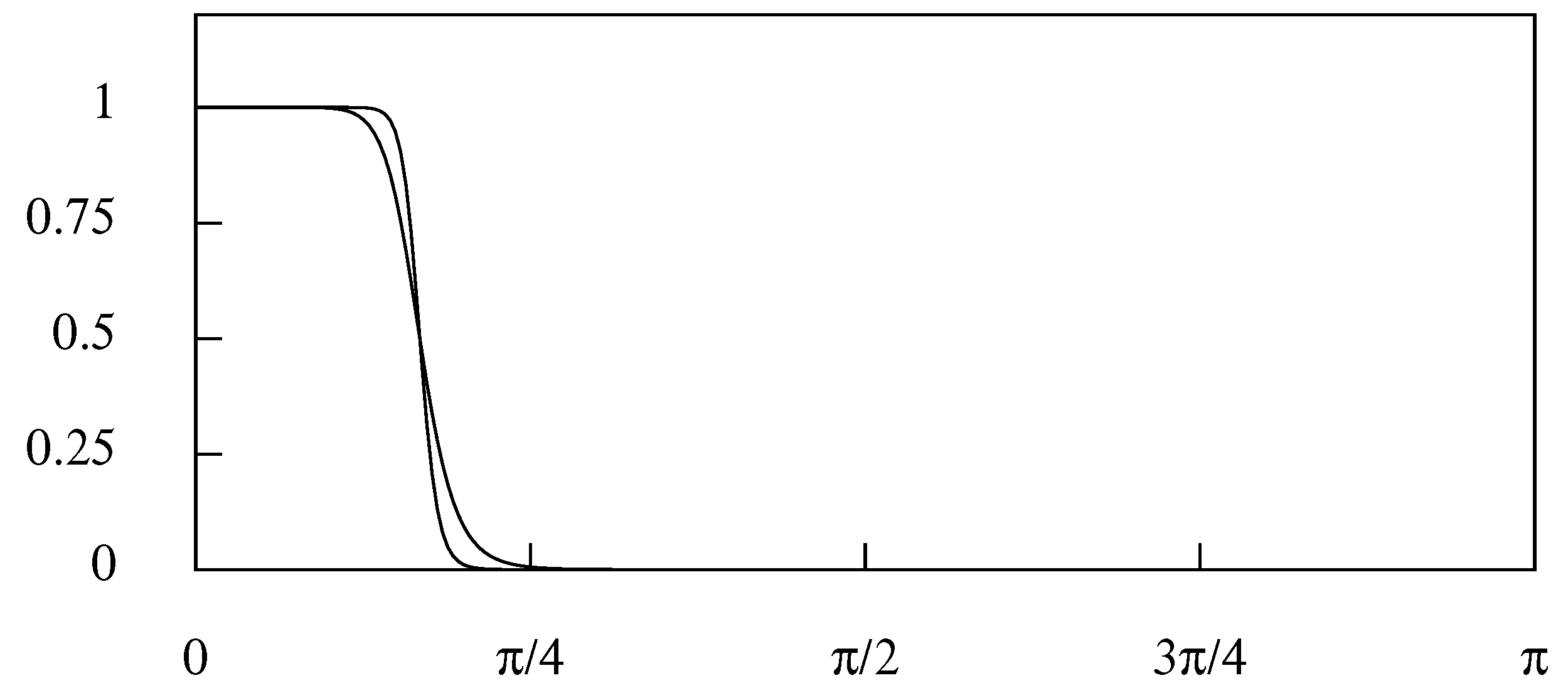
The parameter n, which denotes the order of the filter, is used to govern the rate of transition between the pass band and the stop band. The rate of transition increases as the value of n increases. This is illustrated in Figure 15.

Whereas n must take a positive integer value in the time-domain versions of the filter, it can be a positive real number in the frequency-domain versions, which employ the functions ${\psi }_L(\omega )$ and ${\psi }_H(\omega )$ to rescale the Fourier ordinates of the data.

5.4. The Hodrick–Prescott Filter

A Wiener–Kolmogorov filter that is commonly deployed in econometric analyses is one that has been attributed to Hodrick and Prescott (1980, 1997), which should also be attributed to Leser (1961), who provided an earlier exposition.

In terms of the structures of Equations (45) and (46), the filter is specified by setting

$${\delta }_L(z)=1\mathrm{and}{\delta }_H(z)={\lambda }^{1/2}{(1-z)}^2.$$

(53)

The resulting low pass and high pass versions are

$${\psi }_L(z)=\frac{1}{1+\lambda {(1-z^{-1})}^2{(1-z)}^2}\mathrm{and}{\psi }_H(z)=\frac{\lambda {(1-z^{-1})}^2{(1-z)}^2}{1+\lambda {(1-z^{-1})}^2{(1-z)}^2},$$

(54)

whereas their frequency response functions, which depend on the results of (A5) in Appendix A, are

$${\psi }_L(z)=\frac{1}{1+\lambda {\{2sin(\omega /2)\}}^4}\mathrm{and}{\psi }_H(z)=\frac{\lambda {\{2sin(\omega /2)\}}^4}{1+\lambda {\{2sin(\omega /2)\}}^4}.$$

(55)

In common with the Butterworth filter, the Hodrick–Prescott filter must be allied to a method for coping with short trended data sequences, if it is to be fully adapted for econometric circumstances. Two such adaptations are described in the sequel, which are appropriate, respectively, to the frequency-domain and the time-domain implementations of the filters.

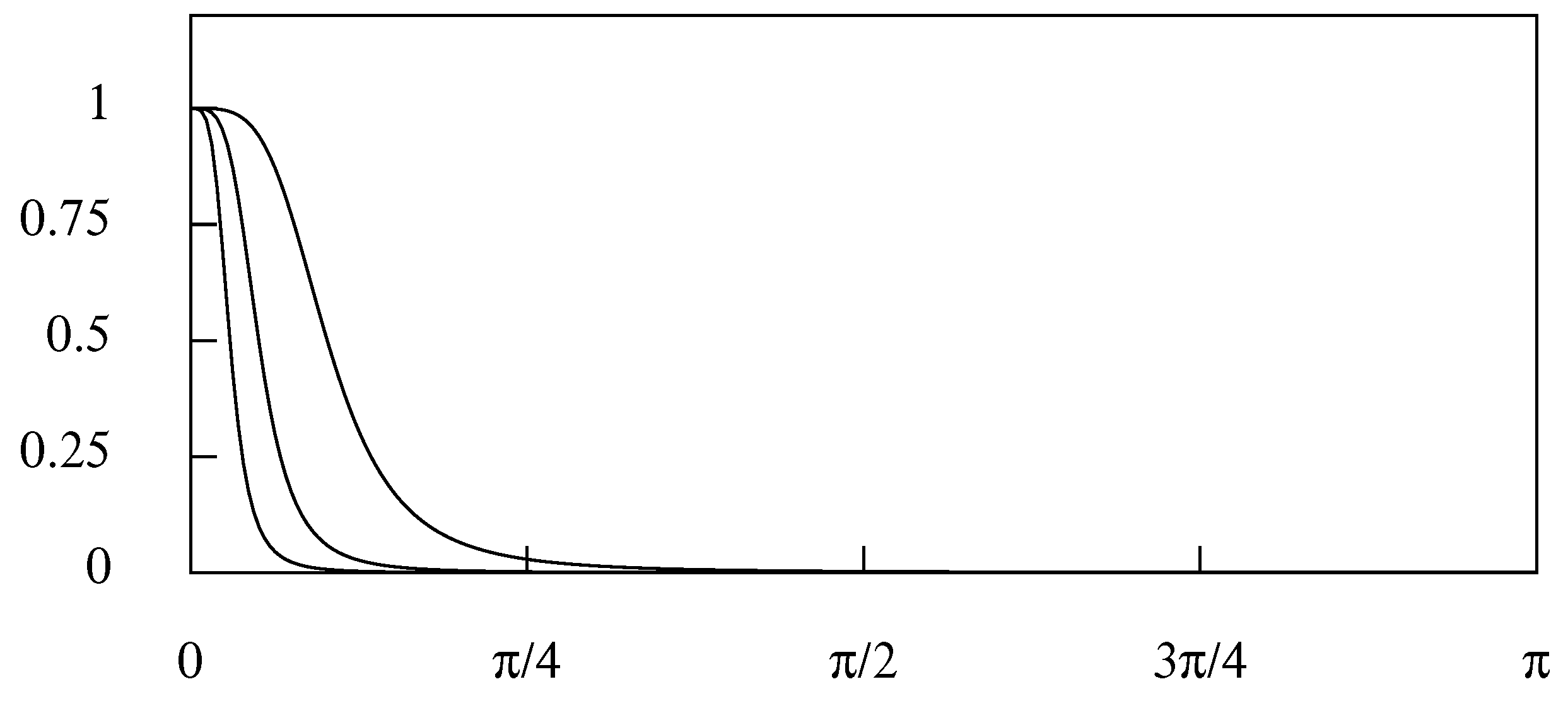
The Hodrick–Prescott filter has been used as a low pass smoothing filter in numerous macroeconomic investigations, where it has been customary to set the smoothing parameter to certain conventional values. Thus, for example, the econometric computer package Eviews 4.0 (QMS 2000) imposes the following default values:

$$\lambda =\left\{\begin{array}{cc}100& \mathrm{for}\mathrm{annual}\mathrm{data},\hfill \\ 1600& \mathrm{for}\mathrm{quarterly}\mathrm{data},\hfill \\ \mathrm{14,400}& \mathrm{for}\mathrm{monthly}\mathrm{data}.\hfill \end{array}\right.$$

(56)

Figure 16 shows the square gain of the filter corresponding to these values. The innermost curve corresponds to $\lambda =\mathrm{14,400}$ and the outermost curve to $\lambda =100$.

Whereas they have become conventional, these values are arbitrary. The filter should be adapted to the purpose of isolating the component of interest; and the appropriate filter parameters need to be determined in the light of the spectral structure of that component, such as has been revealed in Figure 13, in the case of the U.K. consumption data.

It will be observed that a Hodrick–Prescott filter with $\lambda =1600$, which defines the middle curve in Figure 16, will not be effective in isolating the low-frequency component of the quarterly consumption data of Figure 13, which lies in the interval $[0,\pi /8]$. The curve will cut through the low-frequency spectral structure that is represented in Figure 13; and the effect will be greatly to attenuate some of the elements of the component that should be preserved intact.

Lowering the value of $\lambda$ in order to admit a wider range of frequencies will create a frequency response with a gradual transition from the pass band to the stop band. This will be equally inappropriate to the purpose of isolating a component within a well-defined frequency band; and a different filter is required.

For this purpose, a filter with a rapid transition and a well-placed cut-off frequency is needed. The requirement can be particularly stringent in the case of monthly data affected by seasonal variations. Then, the fundamental seasonal frequency is likely to be close to the upper limit of the business-cycle frequencies; and a sharp cut between the two is called for. In that case, an ideal frequency-domain filter or a Butterworth filter with of a high order may serve the purpose.

6. Adapting the Filters to Short and Trended Data

The typical econometric data sequence is of a limited duration, and it may also show a marked trend. The theory of filtering typically presupposes that the data are generated by a statistically homogeneous process of infinite duration that shows no trends. Some significant adaptations are required in order to accommodate the econometric realities.

6.1. Extrapolations of the Data

The methods for adapting the Henderson FIR filters to trended data have been discussed in Section 3. In the case of data that are deemed to have been generated by a statistically stationary mean-zero process, it may be appropriate to proxy the extra-sample elements by their zero-valued unconditional expectations.

In the case of a process embodying a first-order random walk—attributable to a single unit root within an autoregressive operator—it may be appropriate to extrapolate the data at the levels of the end points. This is the basis of a method proposed by Christiano and Fitzgerald (2003).

A more careful procedure that can be followed in the case of trend-free data is to reflect the data around the endpoints to create m extra-sample points at each end, sufficient to enable the filter to generate values $x_0$ and $x_{T-1}$ to replace the data values $y_0$ and $y_{T-1}$. A taper can also be applied to these extrapolations whereby they should converge towards zero. This is a procedure to follow whenever the values at the end points are significantly different from their zero expectations.

An alternative and an equivalent recourse is to fold back the filter coefficients that would otherwise extend beyond the ends of the sample and to add them to the coefficients that lie within the sample. Thus, for example, in the case of $m=3$, the following filters would be applied at the upper end of the sample:

$$\begin{array}{c}\hfill \begin{array}{ccc}\varphi (z)& =& {\varphi }_3{z}^{-3}+{\varphi }_2{z}^{-2}+{\varphi }_1{z}^{-1}+{\varphi }_0+{\varphi }_1{z}^1+{\varphi }_2{z}^2+{\varphi }_3{z}^3,\hfill \\ {\varphi }_{(1)}(z)& =& {\varphi }_2{z}^{-2}+(\lambda {\varphi }_1+{\varphi }_3)z^{-1}+{\varphi }_0+{\varphi }_{1}z+{\varphi }_1{z}^2+{\varphi }_2{z}^3,\hfill \\ {\varphi }_{(2)}(z)& =& {\varphi }_1{z}^{-1}+(\lambda {\varphi }_0+{\varphi }_2)+({\lambda }^2{\varphi }_1+{\varphi }_3)z+{\varphi }_2{z}^2+{\varphi }_2{z}^3,\hfill \\ {\varphi }_{(3)}(z)& =& {\varphi }_0+(1+\lambda ){\varphi }_{1}z+(1+{\lambda }^2){\varphi }_2{z}^2+(1+{\lambda }^3){\varphi }_3{z}^3.\hfill \end{array}\end{array}$$

(57)

Here, $\lambda \in [0,1]$ is the factor that imposes a taper on the folded coefficients.

The first of these expressions represents the ordinary symmetric filter that looks equally back and forwards in time, whereas the last of them, which represents the final filter, looks only back in time. At the lower end, a similar set of filters would be applied, but with z interchanged with $z^{-1}$.

The end-of-sample problem is liable to affect filters that are applied in the frequency domain to no lesser extent than those that are applied in the time domain. This is notwithstanding the fact that the implicit circularity of the data allows filtered values to be generated at both ends of the sample.

In creating the circular data sequence, the head of the sample is joined to its tail, and the extra-sample points at the beginning of the sample are proxied by values from the end of the sample, and vice versa. However, there may a significant difference between the values at the head and the tail, leading to a radical disjunction in the circular data at the point where they are joined.

This circumstance justifies the addition of tapered extrapolations to both ends of the sample. To avoid a disjunction in the circular sequence, the two extrapolations should reach the same value at their furthest points. This can be a achieved using the weights

$$w_j=0.5cos\{1+\pi j/(N+1)\};j=0,1,\dots ,N+1,$$

(58)

which descend from unity when $j=0$, which marks an endpoint of the sample, to zero when $j=N+1$, which marks the terminal point of the extension.

In the case of data that have an evolving pattern of seasonal variation, Pollock (2016) has proposed to interpolate into the circular data sequence, at the point of the juncture, a synthetic data sequence in which the seasonal pattern of the final years is gradually transformed into the pattern of the initial years. The transformation is by virtue of a weighted average of the two patterns, wherein the evolving weights are governed by a logistic curve based on the half-cycle of a cosine function. An example is provide by Figure 17.

6.2. The Interpolation of a Trend Function

There are two common methods of removing the trend from the data that seem to be very different. The first method relies on the interpolation of a trend function, which is commonly a polynomial function, by a method of least-squares regression. The end-of-sample problem can be alleviated by attributing extra weight to the data at the ends of the sample in order to bring them and the regression line closer together. Then, there can be more justification for using zeros as proxies for the extra-sample elements.

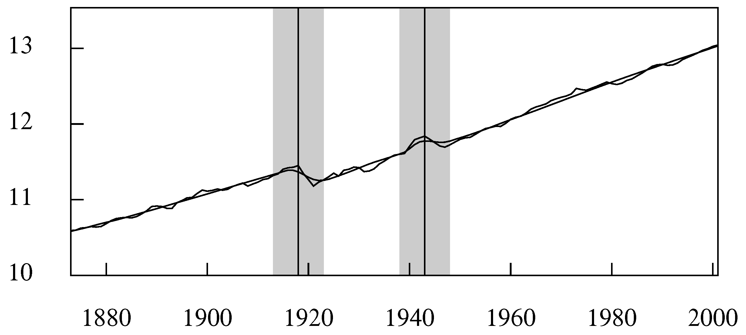
A trend can also be interpolated into the data by the Hodrick–Prescott filter, with a high degree of smoothing. A version of Hodrick–Prescott filter with a smoothing parameter that is allowed to vary over the length of the data has also been provided by Pollock (2016). By setting the smoothing parameter to a low value in the vicinity, a so-called structural break in the data can be absorbed by the trend, which maintains its stiffness in other regions (see Figure 18).

Once the data have been subjected to a preliminary detrending, the residual sequence can be subjected to the filtering procedures that are applicable to non-trended data. If this is a low pass filtering, designed to isolate the low-frequency cycles of the data, then the filtered sequence can be added to the estimated trend to create a trend-cycle trajectory.

6.3. The Differencing and Anti-Differencing in the Time Domain

Another common way of removing the trend from the data sequence is to apply a differencing operator. Usually, a twofold differencing operator is appropriate, which will serve to reduce a linear trend to zero. In the case of backward differences, the twofold operator takes the form of

$${\nabla }^2(z)={(1-z)}^2=1-2z+z^2.$$

(59)

The matrix form of the operator, which is applicable to a finite data vector $y={[y_0,y_1,\dots ,y_{T-1}]}^{\prime }$, is illustrated, in the case of $T=5$, by

$${\nabla }_5^2=\left[\begin{array}{c}{Q}_{*}^{\prime }\\ Q^{\prime }\end{array}\right]=\left[\begin{array}{ccccc}1& 0& 0& 0& 0\\ -2& 1& 0& 0& 0\\ 1& -2& 1& 0& 0\\ 0& 1& -2& 1& 0\\ 0& 0& 1& -2& 1\end{array}\right].$$

(60)

The first two rows, which do not produce true differences, are liable to be discarded.

The twice differenced sequence can be filtered and then it can be re-inflated or anti-differenced with the help of the twofold summation operator, which is

$${\Sigma }^2(z)={(1-z)}^{-2}=\{1+2z+3z^2+\cdots \}.$$

(61)

The matrix version of the operator for $T=5$ is

$${\Sigma }_5^2=\left[\begin{array}{cc}{S}_{*}& S\end{array}\right]=\left[\begin{array}{ccccc}1& 0& 0& 0& 0\\ 2& 1& 0& 0& 0\\ 3& 2& 1& 0& 0\\ 4& 3& 2& 1& 0\\ 5& 4& 3& 2& 1\end{array}\right].$$

(62)

The twofold summation operator must be accompanied by two initial conditions to compensate for the loss of two data points in forming the vector $d=Q^{\prime }y$ of second differences. If a low pass filter with a unit gain at zero frequency has been applied, then the initial conditions should be determined such as to bring the re-inflated sequence into as close an alignment as possible with the data. The same criterion is applied in finding the initial conditions for the re-inflation of the complementary high pass component.

Let x and h be, respectively, the low pass and the high pass component of the data vector $y=x+h$. These must be recovered from their differenced versions $g=Q^{\prime }x$ and $k=Q^{\prime }h$, which are the components of the vector $d=Q^{\prime }y=g+k$ that is subject to the filtering. The recovered vectors are

$$x=S_{*}{d}_{*}+Sd\mathrm{where}{d}_{*}={(S_{*}^{\prime }{S}_{*})}^{-1}{S}_{*}^{\prime }(y-Sd)$$

(63)

and

$$h=S_{*}{k}_{*}+Sk\mathrm{where}{k}_{*}=-{(S_{*}^{\prime }{S}_{*})}^{-1}{S}_{*}^{\prime }Sk.$$

(64)

Here, $d_{*}$ and $k_{*}$ are the initial conditions that are obtained via the minimisation of the function

$$\begin{array}{c}\hfill \begin{array}{ccc}{(y-x)}^{\prime }(y-x)& =& {(y-S_{*}{d}_{*}-Sd)}^{\prime }(y-S_{*}{d}_{*}-Sd)\hfill \\ & =& {(S_{*}{k}_{*}+Sk)}^{\prime }(S_{*}{k}_{*}+Sk)=h^{\prime }h,\hfill \end{array}\end{array}$$

(65)

which ensures that the estimated trend x adheres as closely as possible to the data y.

In the case where the data are differenced twice, there is

$$S_{*}^{\prime }=\left[\begin{array}{ccccc}1& 2& \dots & T-1& T\\ 0& 1& \dots & T-2& T-1\end{array}\right].$$

(66)

The elements of the matrix $S_{*}^{\prime }{S}_{*}$ can be found via the formulae

$$\begin{array}{ccc}\hfill \sum _{t=1}^T{t}^2& =& \frac{1}{6}T(T+1)(2T+1)\mathrm{and}\hfill \\ \hfill \sum _{t=1}^{T}t(t-1)& =& \frac{1}{6}T(T+1)(2T+1)-\frac{1}{2}T(T+1).\hfill \end{array}$$

(67)

A compendium of such results has been provided by Jolly (1961), and proofs of the present results were given by Hall and Knight (1899).

6.4. Centralised Differences

The elimination of the trend can also be accomplished by a centralised operator of the form

$$\Gamma (z)=(1-z^{-1})(1-z)=-z^{-1}{\nabla }^2(z).$$

(68)

The frequency-response function of the operator, which is obtained by setting $z=exp\{-\mathrm{i}\omega \}$ in this equation, and by invoking the result (A5) of Appendix A, is

$$\Gamma (\omega )=2-2cos(\omega )={\{2sin(\omega /2)\}}^2.$$

(69)

This is zero at zero frequency. The frequency response of the anti-differencing operator ${\Gamma }^{-1}(\omega )$ has an indefinite value at zero frequency,

The matrix version of the centralised operator can be illustrated by the case where $T=5$:

$${\Gamma }_5=\left[\begin{array}{c}{n}_0^{\prime }\\ -Q^{\prime }\\ n_4^{\prime }\end{array}\right]=-\left[\begin{array}{ccccc}-2& 1& 0& 0& 0\\ 1& -2& 1& 0& 0\\ 0& 1& -2& 1& 0\\ 0& 0& 1& -2& 1\\ 0& 0& 0& 1& -2\end{array}\right].$$

(70)

In applying this operator to the data, the first and the last elements of ${\Gamma }_{T}y$, which are $n_0^{\prime }y=-2y_0+y_1$ and $n_{T-1}^{\prime }y=y_{T-2}-2_{T-1}$, respectively, are not true differences. Therefore, they are discarded to leave $-Q^{\prime }y={[q_1,\dots ,q_{T-2}]}^{\prime }$. To compensate for this loss, appropriate values are attributed to $q_0$ and $q_{T-1}$, which are formed from combinations of the adjacent values, to create a vector of order T denoted by $q={[q_0,q_1,\dots ,q_{T-2},q_{T-1}]}^{\prime }$.

6.5. The Binomial Filter with Trended Data

The centralised difference operator can be used in conjunction with the binomial filter. The operator is used to eliminate a trend in the data, whereafter the complementary high pass filter is applied to the differenced data.

The z-transform of the high pass filter is

$$1-b_n(z)=1-\frac{{(1+z^{-1})}^m{(1+z)}^m}{2^n}.$$

(71)

This can be compounded with the anti-differencing operator ${\Gamma }^{-1}(z)$, which is the inverse of the difference operator, to create a reduced filter

$$r_n(z)=\frac{1-b_n(z)}{\Gamma (z)}=\frac{1-2^{-n}{(1+z^{-1})}^m{(1+z)}^m}{(1-z^{-1})(1-z)}.$$

(72)

Whereas $b_n(z)$ has zeros at the Nyquist frequency of $\pi$ the complementary high pass filter $1-b_n(z)$ has zeros at zero frequency. These will serve to nullify the unbounded inflationary effect of ${\Gamma }^{-1}(z)$ at zero.

The frequency response function of the compound filter is

$$r_n(\omega )=\frac{1-b_n(\omega )}{\Gamma (\omega )}=\frac{1-{\{cos(\omega /2)\}}^n}{{\{2sin(\omega /2)\}}^2}.$$

(73)

When the filter is applied to the differenced data, it will create a high pass component, which can be subtracted from the data to create the low pass component.

Apart from the initial application of the centralised difference operator, which will be in the time domain, the essential processing can take place in either domain. In the frequency-domain implementation, a Fourier transform must be applied to the diffenced data, whereafter the weighting function of (73) will be applied to the Fourier ordinates. Then, the results will be translated back to the time domain by an inverse Fourier transform.

6.6. The Wiener–Kolmogorov Frequency-Domain Filters with Trended Data

The phase-neutral frequency response of the anti-differencing operator ${\Gamma }^{-1}(\omega )$ can be applied in the frequency domain in conjunction with a high pass filter that operates in that domain, provided that the filter has multiple zeros at zero frequency.

An example is provided by the Butterworth filter. The product of the frequency response of the high pass filter with that of the anti-differencing operator is

$$r(\omega )=\frac{1}{[1+{\lambda }^{-1}{\{\mathrm{cotan}(\omega /2)\}}^{2n}]{\{2sin(\omega /2)\}}^2}.$$

(74)

This function can be used to rescale the ordinates of the Fourier transform of the differenced data. The product can then be subjected to an inverse Fourier transform to carry it into the time domain, and the result can be subtracted from the data to create the low pass component.

A similar procedure can be followed in the case of the Hodrick–Prescott filter, for which the product of the frequency response of the high pass filter with that of the anti-differencing operator is

$$r(\omega )=\frac{\lambda {\{2sin(\omega /2)\}}^2}{1+\lambda {\{2sin(\omega /2)\}}^4}.$$

(75)

7. The Finite-Sample Time-Domain Wiener–Kolmogorov Filters

An alternative to applying the Wiener–Kolmogorov filter in the frequency domain is to adopt a procedure that remains strictly within the time domain. Such an approach has been expounded in detail by Pollock (2007). The minimum mean-square-error filters can be derived, variously, according a least-squares criterion, a maximum-likelihood criterion and a conditional expectations criterion, which are equivalent.

The filters that are appropriate to statistically stationary data are recognisable variants of the filters depicted in Equations (48) and (49), in which the difference and summation operators are replaced by matrix analogues. The filters for trended data that can be reduced to stationarity by twofold differencing are more complicated.

The low pass component of the trended data that is isolated by the Hodrick–Prescott filter is

$$x=y-Q{({\lambda }^{-1}I+Q^{\prime }Q)}^{-1}{Q}^{\prime }y,$$

(76)

where $\lambda$ is the smoothing parameter. The filter is formed by subtracting the high pass filter from the identity matrix.

As $\lambda \to \infty$, the vector x tends to that of a linear function interpolated into the data by least-squares regression, which is represented by the equation $x=y-Q{(Q^{\prime }Q)}^{-1}{Q}^{\prime }y$.

The Butterworth filter that is appropriate to short trended sequences produces the following low pass component:

$$x=y-WQ{(Q^{\prime }WQ+{\lambda }^{-1}M)}^{-1}{Q}^{\prime }y.$$

(77)

Here, the matrices

$$W={\{2I_T-(L_T+L_T^{\prime })\}}^{n-2}\mathrm{and}M={\{2I_T+(L_T+L_T^{\prime })\}}^n$$

(78)

are obtained from the RHS of the equations ${\{(1-z)(1-z^{-1})\}}^{n-2}={\{2-(z+z^{-1})\}}^{n-2}$ and ${\{(1+z)(1+z^{-1})\}}^n={\{2+(z+z^{-1})\}}^n$, respectively, by replacing z by $L_T$ and $z^{-1}$ by $L_T^{\prime }$, where $L_T=[e_1,e_2,\dots ,e_{T-1},0]$ is the matrix lag operator of order T, which is obtained from the identity matrix $I_T=[e_0,e_1,\dots ,e_{T-1}]$ by deleting the first column and by appending a column of zeros at the end.

Observe that the equalities no longer hold after the replacements. However, it can be verified that

$$Q^{\prime }WQ={\{2I_T-(L_T+L_T^{\prime })\}}^n.$$

(79)

One may also observe that the high pass Wiener–Kolmogorov filters for trended data give the same results whether they are applied to the original data or to the residuals from a linear detrending that are contained in the vector $d=Q{(Q^{\prime }Q)}^{-1}{Q}^{\prime }y$. This follows since $Q^{\prime }d=Q^{\prime }y$.

It is also clear that the residual vector contains the same information as the vector of the second differences. Thus, linear detrending and differencing, which appear to be very different ways of removing a trend, can lead to the same results.

The virtue of the finite-sample Wiener–Kolmogorov filters is that they avoid the end-of-sample problem by remaining within the sample and by adapting the filter coefficients continuously according to their location.

Figure 19 shows a sequence of filter coefficients from a finite-sample low pass Butterworth filter of order $n=6$ and with a cut off point at ${\omega }_c=\pi /8$ radians or $22.5^{\circ }$. The size of the sample is $T=51$ and the filtered value is dated by $t=15$.

It can be seen from Equation (77) that the filter matrix is not symmetric. Therefore, the filter coefficients of the tth row will differ from the coefficients in the tth column, which correspond to the response to an impulse at time t. The differences are only significant in small samples.

8. Conclusions

The filters that are commonly deployed in econometric analyses operate exclusively in the time-domain. They often require complicated data extrapolations to cope with the end-of-sample problems that arise when the data are trended. There is much doubt and dispute over the criteria that should inform the design of time-domain econometric filters.

In this paper, it has been proposed that the filters should be designed with reference to their frequency responses. In that case, it is natural that they should also be implemented in the frequency domain. To do so requires that the data should be free of trends. This can be achieved in a variety of ways that have been described in the paper. Working with trend-free data alleviates the end-of-sample problem. Alternative means of restoring the trends after the trend-free data have been processed have also been described.

The methods and procedures that have been discussed in the paper have been implemented in a program called IDEOLOG, which is available, together with its code in Pascal, at the address http://www.le.ac.uk/users/dsgp1/. The program facilitates the comparison of different filters. It includes some filters of which the use has been derogated by the author. (For a critique of some of these filters, see Pollock 2014 and Pollock 2016).

Several of the filters have been implemented in the program both in the time domain and in the frequency domain. Given the equivalence of the results, the user should be indifferent regarding the choice of which version to use. However, it can be argued that, from the point of view of a theory of filtering and for ease of implementation, the frequency-domain versions are to be preferred.

References

- Abramovich, Felix, Trevor C. Bailey, and Theofanis Sapatinas. 2000. Wavelet Analysis and its Statistical Applications. Journal of the Royal Statistical Society: Series D (The Statistician) 49: 1–29. [Google Scholar] [CrossRef] [Green Version]
- Baxter, Marianne, and Robert G. King. 1999. Measuring Business Cycles: Approximate Band-Pass Filters for Economic Time Series. Review of Economics and Statistics 81: 575–93. [Google Scholar] [CrossRef]
- Burns, Arthur F., and Wesley C. Mitchell. 1946. Measuring Business Cycles. New York: National Bureau of Economic Research. [Google Scholar]
- Christiano, Lawrence J., and Terry J. Fitzgerald. 2003. The Band-pass Filter. International Economic Review 44: 435–65. [Google Scholar] [CrossRef]
- Cooley, James W., and John W. Tukey. 1965. An Algorithm for the Machine Calculation of Complex Fourier Series. Mathematics of Computation 19: 297–301. [Google Scholar] [CrossRef]
- Doherty, Mike. 2001. The Surrogate Henderson Filters in X-11. Australian and New Zealand Journal of Statistics 43: 385–92. [Google Scholar] [CrossRef]
- Fishman, George S. 1969. Spectral Methods in Econometrics. Cambridge: Harvard University Press. [Google Scholar]
- Granger, Clive William John, and Michio Hatanaka. 1964. Spectral Analysis of Economic Time Series. Princeton: Princeton University Press. [Google Scholar]
- Gray, Alistair G., and Peter J. Thomson. 2002. On a Family of Finite Moving-average Trend Filters for the Ends of Series. Journal of Forecasting 21: 125–49. [Google Scholar] [CrossRef]
- Guerlac, Henry. 1947. Radar in World War II. Volume 1 of MIT Radiation Laboratory Series; New York: McGraw-Hill. [Google Scholar]
- Hall, Henry Sinclair, and Samuel Ratcliffe Knight. 1899. Higher Algebra. London: Macmillan and Co. [Google Scholar]
- Henderson, Robert. 1916. Note on Graduation by Adjusted Average. Transactions of the Actuarial Society of America 17: 43–48. [Google Scholar]
- Henderson, Robert. 1924. A New Method of Graduation. Transactions of the Actuarial Society of America 25: 29–40. [Google Scholar]
- Hodrick, Robert J., and Edward C. Prescott. 1980. Postwar U.S. Business Cycles: An Empirical Investigation, Working Paper. Pittsburgh: Carnegie Mellon University.
- Hodrick, Robert J., and Edward C. Prescott. 1997. Postwar U.S. Business Cycles: An Empirical Investigation. Journal of Money, Credit and Banking 29: 1–16. [Google Scholar] [CrossRef]
- Henney, Keith, ed. 1953. Index, Volume 28 of MIT Radiation Laboratory Series. New York: McGraw-Hill. [Google Scholar]
- Jolly, Leonard Benjamin William. 1961. Summation of Series: Second Revised Edition. New York: Dover Publications. [Google Scholar]
- Kailath, Thomas. 1974. A View of Three Decades of Filtering Theory. IEEE Transactions on Information Theory 20: 146–81. [Google Scholar] [CrossRef]
- Kenny, Peter B., and James Durbin. 1982. Local Trend Estimation and Seasonal Adjustment of Economic and Social Time Series. Journal of the Royal Statistical Society Series A 145: 1–41. [Google Scholar] [CrossRef]
- Kolmogorov, Andrei Nikolaevitch. 1941. Stationary Sequences in a Hilbert Space. Bulletin of the Moscow State University 2: 1–40. (In Russian). [Google Scholar]
- Kolmogorov, Andrei Nikolaevitch. 1941. Interpolation and Extrapolation. Bulletin de l’Academie des Sciences de U.S.S.R Series Mathematical 5: 3–14. [Google Scholar]
- Kovačević, Jelena, Vivek K. Goyal, and Martin Vetterli. 2013. Fourier and Wavelet Signal Processing. Available online: www.fourierandwavelets.org (accessed on 23 July 2018).
- Ladiray, Dominique, and Benoit Quenneville. 2001. Seasonal Adjustment with the X-11 Method. Springer Lecture Notes in Statistics 158. Berlin: Springer Verlag. [Google Scholar]
- Laniel, Normand. 1986. Design Criteria for 13-Term Henderson End-Weights. Technical Report Working paper TSRA-86-011. Ottawa: Statistics Canada. [Google Scholar]
- Leser, C. E. V. 1961. A Simple Method of Trend Construction. Journal of the Royal Statistical Society, Series B 23: 91–107. [Google Scholar]
- Mallat, Stéphane. 1998. A Wavelet Tour of Signal Processing. San Diego: Academic Press. [Google Scholar]
- Musgrave, J. C. 1964a. A Set of End Weights to End all End Weights, Unpublished Working Paper of the U.S. Bureau of Commerce.
- Musgrave, J. C. 1964b. Alternative Sets of Weights Proposed for X-11 Seasonal Factor Curve Moving Averages, Unpublished Working Paper of the U.S. Bureau of Commerce.
- Nahin, Paul J. 2006. Dr. Euler’s Fabulous Formula. Princeton: Princeton University Press. [Google Scholar]
- Nyquist, Harry. 1928. Certain Topics in Telegraph Transmission Theory. AIEE Transactions, Series B 47: 617–44. [Google Scholar] [CrossRef]
- Oppenheim, Alan V., and Ronald W. Schafer. 1975. Digital Signal Processing. Englewood: Prentice-Hall. [Google Scholar]
- Pollock, D. Stephen G. 2007. Wiener–Kolmogorov Filtering, Frequency-Selective Filtering and Polynomial Regression. Econometric Theory 23: 71–88. [Google Scholar] [CrossRef]
- Pollock, D. Stephen G. 2008. Realisations of Finite-Sample Frequency Selective Filters. Journal of Statistical Planning and Inference 139: 1541–58. [Google Scholar] [CrossRef]
- Pollock, D. Stephen G. 2009. Statistical Signal Extraction and Filtering: A Partial Survey. In Handbook of Computational Econometrics. Edited by David Belsley and Erricos Kontoghiorges. Chichester: John Wiley and Sons, chp. 9. pp. 321–76. [Google Scholar]
- Pollock, D. Stephen G. 2014. Cycles, Syllogisms and Semantics: Examining the Idea of Spurious Cycles. Journal of Times Series Econometrics 6: 81–102. [Google Scholar] [CrossRef]
- Pollock, D. Stephen G. 2016. Econometric Filters. Computational Economics 48: 669–91. [Google Scholar] [CrossRef]
- Rabiner, Lawrence R., and Bernard Gold. 1975. Theory and Application of Digital Signal Processing. Englewood: Prentice-Hall. [Google Scholar]
- QMS. 2000. Eviews 4.0. Irvine: Quantitative Micro Software (QMS). [Google Scholar]
- Ridenour, Louis Nicot. 1947. Radar System Engineering, Volume 1 of MIT Radiation Laboratory Series. New York: McGraw-Hill. [Google Scholar]
- Shannon, Claude Elwood. 1949a. Communication in the Presence of Noise. Proceedings of the Institute of Radio Engineers 37, 10–21. Reprinted in 1998. Proceedings of the IEEE 86: 447–57. [Google Scholar] [CrossRef]
- Shannon, Claude E. 1949b. The Mathematical Theory of Communication. Urbana: University of Illinois Press, Reprinted in 1998. [Google Scholar]
- Shiskin, Julius, Allan H. Young, and John C. Musgrave. 1967. The X-11 Variant of the Census Method II Seasonal Adjustment Program; Technical Paper 15. Washington, D.C.: Bureau of the Census, U.S. Department of Commerce.
- Vetterli, Martin, Jelena Kovacčević, and Vivek K. Goyal. 2014. Foundations of Signal Processing. Available online: www.fourierandwavelets.org (accessed on 23 July 2018).
- Wallis, Kenneth F. 1981. Models for X-11 and X-11-Forecast Procedures for Preliminary and Revised Seasonal Adjustments. Paper presented at the A.S.A–Census–NBER Conference on Applied Time Series Analysis of Economic Data, Washington, D.C., US; pp. 3–11. [Google Scholar]
- Wiener, Norbert. (1941) 1949. Extrapolation, Interpolation and Smoothing of Stationary Time Series. Report on the Services Research Project DIC-6037. Published in book form. Cambridge: MIT Technology Press, New York: John Wiley and Sons. [Google Scholar]
Figure 1.
A diagram to illustrate the effects of aliasing in the process of sampling when there are frequencies beyond the Nyquist range , which defines the innermost circle. Frequencies on the outer circles are mapped onto the inner circle by following the radial lines, e.g. and (The arcs with broken lines correspond to negative frequencies).
Figure 2.
The scaling function . The function continues indefinitely in both directions.
Figure 3.
Figure 4.
The wavelet function .
Figure 5.
The coefficients of the symmetric Henderson filter of 23 points.
Figure 6.
The frequency response function of the Henderson moving-average filter of 23 terms.
Figure 7.
A trend, determined by a Henderson filter with 23 coefficients, interpolated through 160 logarithms of the quarterly household expenditure in the U.K. for the years 1955 to 1994.
Figure 8.
Two representations of the conversion of a low pass filter to a band pass filter by a cosine modulation, which creates two displaced copies of the low pass filter.
Figure 9.
The rectangular frequency response of the ideal band pass filter defined on the interval , together with the frequency response of the truncated filter of 25 coefficients.
Figure 10.
The frequency response of the 16-point wrapped filter defined over the interval . The values at the Fourier frequencies are marked by circles and dots. Note that, when the horizontal axis is wrapped around the circumference of the unit circle, the points at and coincide. Therefore, only one of them is included in the interval.
Figure 11.
The frequency response of the 17-point wrapped filter defined over the interval . The values at the Fourier frequencies are marked by circles.
Figure 12.
The deviations of the logarithms of the index of UK domestic expenditure from an interpolated linear trend. The smooth trajectory, which has been synthesised from the Fourier ordinates of the data that fall in the interval , corresponds to the business cycle.
Figure 13.
The periodogram of logarithmic expenditure data of Figure 12.
Figure 14.
The periodogram of the subsampled anti-aliased data with the parametric spectrum of an estimated AR(2) model superimposed.
Figure 15.
The frequency response function of the Butterworth filters of orders and with a nominal cut-off point of radians .
Figure 16.
The frequency response function of the Hodrick–Prescott low pass smoothing filter—or Leser filter—for various values of the smoothing parameter.
Figure 17.
The residuals from a linear detrending of the logarithms of the monthly U.S. retail sales from January 1953 to December 1964, with an interpolation of four years length inserted between the end and the beginning of the circularised sequence, marked by the shaded band.
Figure 18.
The logarithms of annual U.K. real GDP from 1873 to 2001 with an interpolated trend. The trend is estimated via a filter with a variable smoothing parameter.
Figure 19.
The coefficients from a finite-sample Butterworth filter of order and with a cut-off frequency of . The filter is appropriate to a sample of points and the output is at .
© 2018 by the author. Licensee MDPI, Basel, Switzerland. This article is an open access article distributed under the terms and conditions of the Creative Commons Attribution (CC BY) license (http://creativecommons.org/licenses/by/4.0/).
Share and Cite
MDPI and ACS Style
Pollock, D.S.G. Filters, Waves and Spectra. Econometrics 2018, 6, 35. https://0-doi-org.brum.beds.ac.uk/10.3390/econometrics6030035
AMA Style
Pollock DSG. Filters, Waves and Spectra. Econometrics. 2018; 6(3):35. https://0-doi-org.brum.beds.ac.uk/10.3390/econometrics6030035
Chicago/Turabian StylePollock, D. Stephen G. 2018. "Filters, Waves and Spectra" Econometrics 6, no. 3: 35. https://0-doi-org.brum.beds.ac.uk/10.3390/econometrics6030035
Note that from the first issue of 2016, this journal uses article numbers instead of page numbers. See further details here.