A Prediction Methodology of Energy Consumption Based on Deep Extreme Learning Machine and Comparative Analysis in Residential Buildings

Abstract

In this paper, we have proposed a methodology for energy consumption prediction in residential buildings. The proposed method consists of four different layers, namely data acquisition, preprocessing, prediction, and performance evaluation. For experimental analysis, we have collected real data from four multi-storied residential building. The collected data are provided as input for the acquisition layer. In the pre-processing layer, several data cleaning and preprocessing schemes were deployed to remove abnormalities from the data. In the prediction layer, we have used the deep extreme learning machine (DELM) for energy consumption prediction. Further, we have also used the adaptive neuro-fuzzy inference system (ANFIS) and artificial neural network (ANN) in the prediction layer. In the DELM different numbers of hidden layers, different hidden neurons, and various types of activation functions have been used to achieve the optimal structure of DELM for energy consumption prediction. Similarly, in the ANN, we have employed a different combination of hidden neurons with different types of activation functions to get the optimal structure of ANN. To obtain the optimal structure of ANFIS, we have employed a different number and type of membership functions. In the performance evaluation layer for the comparative analysis of three prediction algorithms, we have used the mean absolute error (MAE), root mean square error (RMSE) and mean absolute percentage error (MAPE). The results indicate that the performance of DELM is far better than ANN and ANFIS for one-week and one-month hourly energy prediction on the given data.

1. Introduction

The energy consumption in residential buildings has significantly increased in the last decade. Energy is an essential part of our lives and almost all things in some way are associated with electricity [1,2]. According to the report issued by the US Energy Information Administration (EIA), 28% growth in global energy demand may occur until 2040 [3]. Due to improper usage, a tremendous amount of energy is wasted annually; hence, energy wastage can be avoided by efficient utilization of energy. Smart solutions are required to certify the proper use of energy [4]. An energy consumption prediction is very significant to achieve efficient energy maintenance and reduce environmental effect [5,6,7]. However, in residential buildings, it is quite challenging as there are many types of buildings and different forms of energy. Also many factors are involved to influence the energy behaviour of the building structures, such as weather circumstances, the physical material used in the building construction, company behaviour, sub-level systems, i.e., lighting, heating, ventilating, and air-conditioning (HVAC) systems, and the execution and routines of the sub-level components [8].

Technologies based on the Internet of Things (IoT) are immensely significant to comprehend the notion of smart homes. Numerous solutions for obtaining energy consumption predictions in buildings based on the IoT can be found in the literature [9]. Energy management and efficiency is the next most crucial area for IoT applications in South Korea [9]. From 2003, homes in this country have been getting smarter and smarter with the inclusion of remote communication devices. The energy demand in South Korea is growing day-by-day; in 2013 South Korea was the eighth largest energy consuming country. The energy consumption distribution in South Korea is between residential and commercial sectors (38%), the industrial sector (55%), the transport sector (1%), and the public sector (6%) [10] as shown in Figure 1.

Many solutions were developed based on machine learning algorithms for energy consumption prediction. These models use historical data, which reflect process behavior to be modeled [11,12]. The machine learning techniques that have been used redundantly for prediction purposes are artificial neural networks [7], adaptive neuro-fuzzy inference system (ANFIS) [13], support vector machine (SVM) [14], extreme learning machine (ELM) [15], and so forth. The ELM method has some advantages over the conventional NNs such as they are easy to use, fast learning, provide good generalization results, can easily be applied, and can get least training inaccuracy and minimum norm of weights [16]. Nowadays the deep learning approaches have also been used in various areas for prediction purposes [17], such as a deep neural network, deep belief network, and a recurrent neural network. The term of deep learning states the number of layers through which data are transferred [18]. The deep learning techniques are powerful tools to obtain healthier modelling and prediction performance. The datasets used in References [18,19,20] for time series prediction applications do not have a large quantity of data as compared to datasets in the research areas of image processing, speech recognition and machine vision. Though, in these applications, the deep learning methods worked efficiently as compared to the conventional machine learning approaches due to their slightly deeper architectures and novel learning methods.

In this paper, we have proposed a methodology for the energy prediction having four layers, i.e., the data acquisition layer, the pre-processing layer, the prediction layer, and the performance evaluation layer. We have performed different operations on the data in each layer of the proposed model. In the prediction layer, we used the deep extreme learning (DELM) approach for the improved performance of the energy consumption prediction. The DELM takes the benefits of both extreme learning and deep learning techniques. The DELM increases the number of hidden layers in the original ELM network structure, arbitrarily initializes the input layer weights and the initial hidden layer weights along with the bias of initial hidden layer, uses the technique for hidden layers (excluding first hidden layer) parameters calculation, and finally uses the least square technique for output network weights calculation. We have used the trial and error method to set the best number of hidden layers, a suitable number of neurons in the hidden layers, and a compatible activation function. The performance evaluation of the proposed DELM model with an adaptive neuro-fuzzy inference system (ANFIS) and artificial neural network (ANN) regarding energy consumption prediction was carried out.

The rest of the paper is organized as follow. The related work is given in Section 2, a detailed explanation of the proposed model comprised of data acquisition, preprocessing, prediction and performance evaluation modules are given in Section 3. Section 4 discusses the experimental results based on prediction algorithms in detail. The discussion and comparative analysis explanation are provided in Section 5. The paper conclusion and future work are discussed in Section 6.

2. Related Work

Energy is an extremely vital resource and its demand is growing day-by-day. Saving energy is not only significant to promote a green atmosphere for future sustainability but also vital for household consumers and the energy production corporations. Electricity affects the user’s regular expenses and the user always wants to decrease their monthly expenses. Energy production companies are always under intense pressure to fulfil the growing energy demand of the commercial and domestic sectors. Techniques for proficient energy consumption prediction are essential for all stakeholders. Many researchers have made numerous efforts and developed several methods for energy consumption prediction.

Generally, we can achieve more accurate results by using machine learning in different real-world applications. Kalogirou [21] approached a back propagation neural network for the required heating load prediction in buildings. The training of the algorithm was carried out for the energy consumption data of 225 buildings; these buildings were different in sizes from small spaces to big rooms. Olofsson [22] proposed a method to forecast the energy requirement on a yearly basis for a small single-family building situated in Sweden. Yokoyama [23] suggested a method for a cooling demand prediction in a building based on the back propagation neural network. Kreider [24] applied a recurrent neural network to predict energy consumption hourly based on the heating and cooling energy prediction in buildings. The recurrent neural network also used by Ben-Nakhi [25] for the cooling load prediction of three office buildings. The data used for model training and testing was collected from 1997 to 2000 for short-term energy prediction. Carpinteiro [26] used a hierarchical neural network based model for short-term energy consumption prediction. They have used two self-organization maps for load forecasting. The Euclidian distance was used to calculate the distance between two vectors. They have used the Brazilian utility dataset for the energy consumption prediction. Their proposed approach performed well for both short-term and long-term forecasting. Another technique was suggested based on a regression model for short-term load forecasting [27]. Irisarri [28] proposed a method of energy load prediction based on summer and winter sessions. Ali, in Reference [29], proposed a technique comprising of six stages for smart homes energy consumption prediction in South Korea. They have used the Kalman filter as a predictor and the Mamdani fuzzy controller to control the actuators. Wahid [30] proposed a technique for energy consumption prediction in residential buildings. They have calculated the first two statistical moments namely mean and variance for the data that consisted of hourly, daily, weekly and monthly energy consumption. Then, the multilayer perceptron on the data with statistical moments was applied for energy consumption prediction. The trial and test methods were used to address a suitable combination of input, hidden, and output layers of neurons. Wahid [31] proposed another energy consumption prediction methodology for residential buildings. The introduced method consisted of five stages, namely data source, data collection, feature extraction, prediction, and performance assessment. Different machine learning algorithms, such as Multi-Layer Perceptron, Random Forest, and K-Nearest Neighbors Algorithms (KNN) were used to obtain the energy consumption predicted results. Arghira [32] presented an energy consumption forecasting method for different appliances in homes. The technique used in this study was developed to predict the day-ahead electricity demand for homes. In this study, the authors have used a historical dataset for homes in France. In this paper, the authors have suggested a stochastic predictor and tested two other predictors. Two pre-processing methods were also proposed namely, segmentation and aggregation. Li [33] suggested an alternate method called the hybrid genetic algorithm-adaptive network-based fuzzy inference system (GA-ANFIS) for energy consumption prediction. In their proposed approach, the GA algorithm was used as an optimizer, which assisted in developing the rule base and the premises and subsequent factors were adjusted through ANFIS for optimization of the prediction performance. Kassa, in Reference [34], proposed a model based on ANFIS for one-day ahead energy generation prediction. The proposed model was tested on real information of a wind power generation profile and the results provided by this method were prominent. In another paper, Ekici [35] proposed a technique using the ANFIS model to predict the energy demands of diverse buildings with different characteristics.

Nowadays, deep learning approaches have been used extensively for energy consumption prediction [18,19,20]. Hence, due to the greater ability of learning, the deep learning (DL) methods have been used to improve the performance of modelling, classification, and visualization problems. Collobert [36] proposed an approach based on a convolutional neural network (CNN) for natural language processing (NLP). Hinton [37] used a deep auto-encoder to reduce the dimensionality and the results indicate that the deep auto-encoder performs better compared to a principal component analysis (PCA). Qiu [20] used a DL technique to predict time series small-batch data sets. Li [18] used a deep learning technique to predict traffic flow based on time series data. After review of all these applications, the results indicate that the performance of deep learning techniques is better compared to other counterpart approaches.

Figure 2 illustrates the proposed conceptual model for energy consumption prediction. The proposed methodology consisted of four main modules, namely data acquisition, pre-processing, prediction, and performance evaluation.

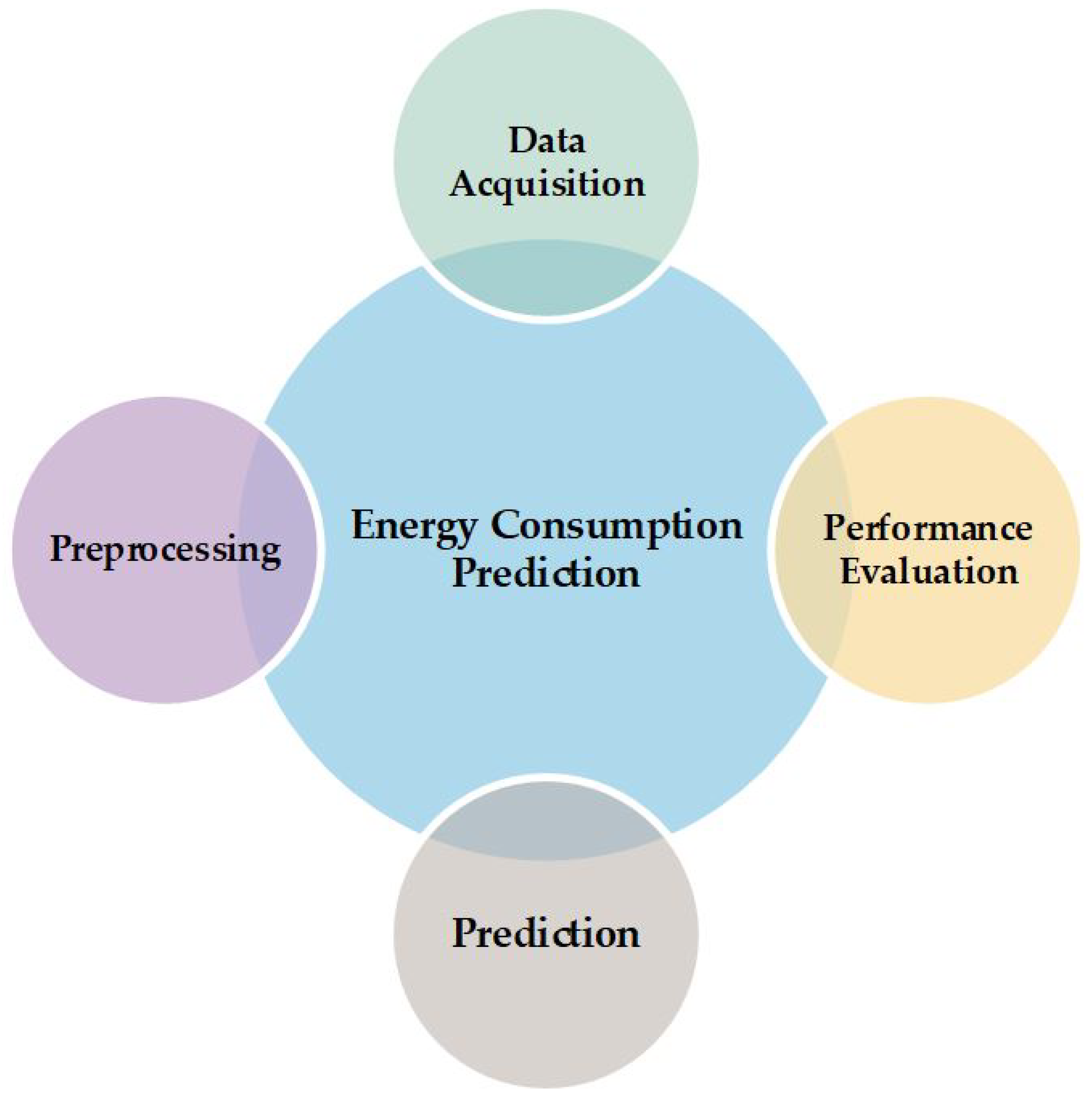
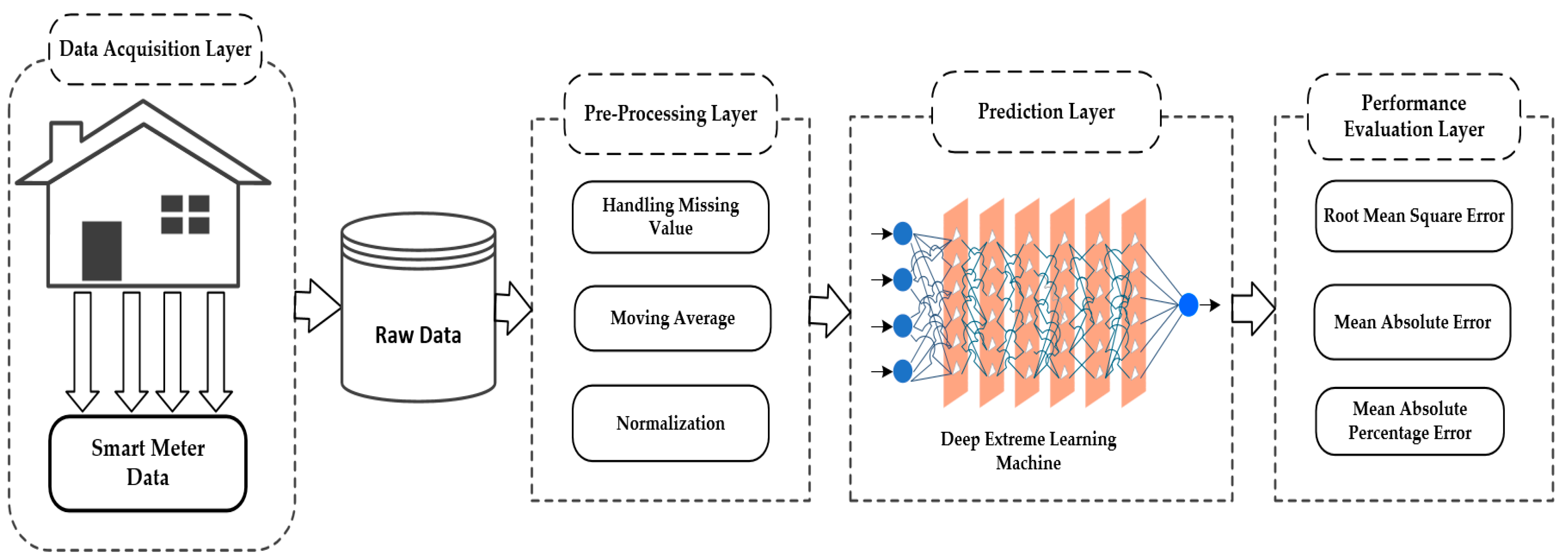
3. Proposed Energy Consumption Prediction Methodology

Energy consumption prediction in residential building is extremely important; it assists the manager to preserve energy and to avoid wastage. Due to the unpredictability and noisy disorder, correct energy consumption prediction in residential buildings is a challenging task. In this paper, we have proposed a methodology based on a deep extreme learning machine (DELM) for energy consumption prediction in residential buildings. We have divided the proposed method into four main layers, namely data acquisition, preprocessing, prediction, and performance evaluation. In the data acquisition layer, we have discussed the detailed data used in the experimental work. In the preprocessing layer, the moving average has been used to remove abnormalities from the data. In the prediction layer, the deep extreme learning machine (DELM) has been proposed to enhance the accuracy of energy consumption results. In the performance evaluation layer, MAE, RMSE, and MAPE [14] performance measures have been used to measure the performance of prediction algorithms. Figure 3 shows the detailed structure of the diagram of the proposed method.

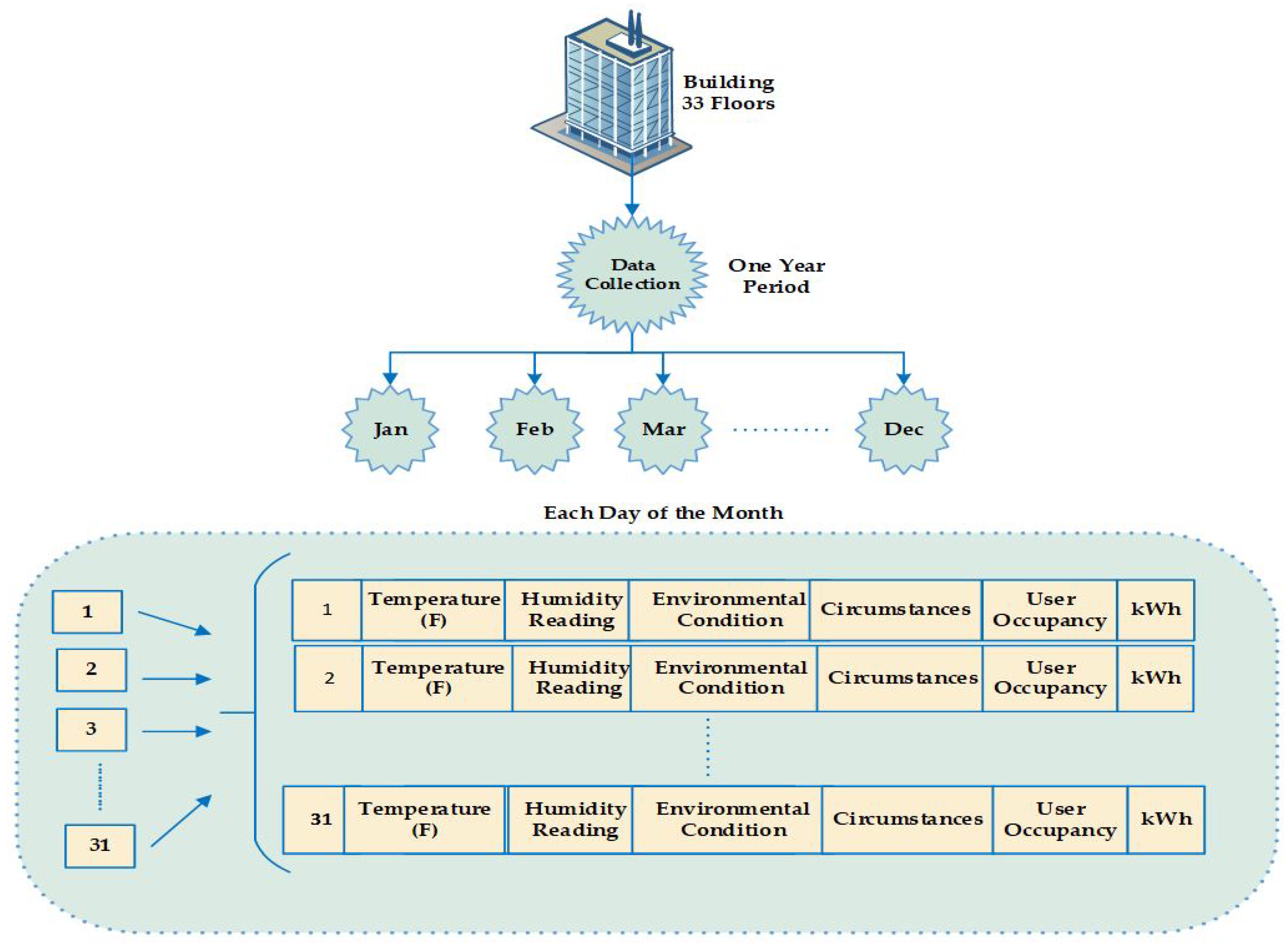
3.1. Data Acquisition Layer

Figure 4 shows the data collection phase. The datasets from four residential buildings from January to December 2010 were collected [10].

We have completed the task of data collection in the data acquisition layer for the proposed work. Sensors were mostly used for the collection of contextual information such as environmental conditions, circumstances, temperature, humidity, user occupancy, and so forth. For user occupancy detection, several Passive Infra-Red (PIR) sensors were used to obtain information in 0, 1 form, such as busy or not busy. To get the information about user occupancy, the installation of cameras in transition positions between several regions of the building was required. The collection of the designated residential buildings data was carried out from January 2010 to December 2010. The building had 33 floors (394 ft. tall), the floor-wise information was collected from smart meters and used for this work. The installations of these meters have been carried out in a floor wise manner in the chosen buildings. It also indicated a direct relationship between energy utilization and users occupancy in the dataset. To better explain the entire energy consumption data, a box plot was used. The x-axis represents the hours of the day (24 h), the y-axis represents the energy consumption in kWh. The box represents the energy consumption in a particular hour of the day for the whole year. The long length box indicates high energy consumption and the short length box indicates low energy consumption. As residential buildings are very busy during noon and night times, the energy consumption was higher during these timings. The entire dataset of hourly energy consumption used in the proposed work is shown in Figure 5 for better observation.

3.2. Preprocessing Layer

In the pre-processing layer, we have removed abnormalities from the data. The data were assumed to have noise due to the inherent nature of data recording where several external aspects affect the reading. In the same way, there were many factors involved in outliers such as meter problem, human mistake, measurement errors, and so forth. Different smoothing filters can be used to remove abnormalities from the data, such as a moving average, loess, lowess, Rloess, RLowess, Savitsky-Golay. In this study, we have used the moving average method, which is an important filter and widely used by various authors [14] for data smoothing. Equation (1) is the mathematical representation of the moving average filter.

$$y\left[i\right]=\frac{1}{\mathrm{M}}{\displaystyle \sum }_{\mathrm{J}=0}^{\mathrm{M}-1}\mathrm{X}\left(\mathrm{i}+\mathrm{j}\right)$$

(1)

where x [ ] represents the inputs, y [ ] denotes the outputs, and M indicates the points of the moving average. In the proposed work, M was equal to 5, which was a suitable size for data smoothing [38].

Usually, data normalization is required when the sample data is scattered and the sample span is large. Hence, the span of the data was minimized for building models and predictions. The normalization was done, in essence, to have the same range of values for each of the inputs to the machine learning models. It can guarantee a stable convergence of weight and biases. In machine learning algorithm modelling for increasing prediction accuracy and for training process improvement, complete sample data were normalized to fit them in the interval [0, 1] by using Equation (2) given below:

$$P=\frac{x_i-x_{min}}{x_{max}-x_{min}},i=1,2,3\dots ,\mathrm{N},$$

(2)

where P represents the mapped values, x denotes the starting value, $x_i$ is i of input data; $x_{max}$ and $x_{min}$ indicate the maximum and minimum values of starting data accordingly [39].

3.3. Prediction Layer

In the prediction layer, we have used three well-known machine learning algorithms to make one-week and one-month energy consumption predictions for the residential buildings.

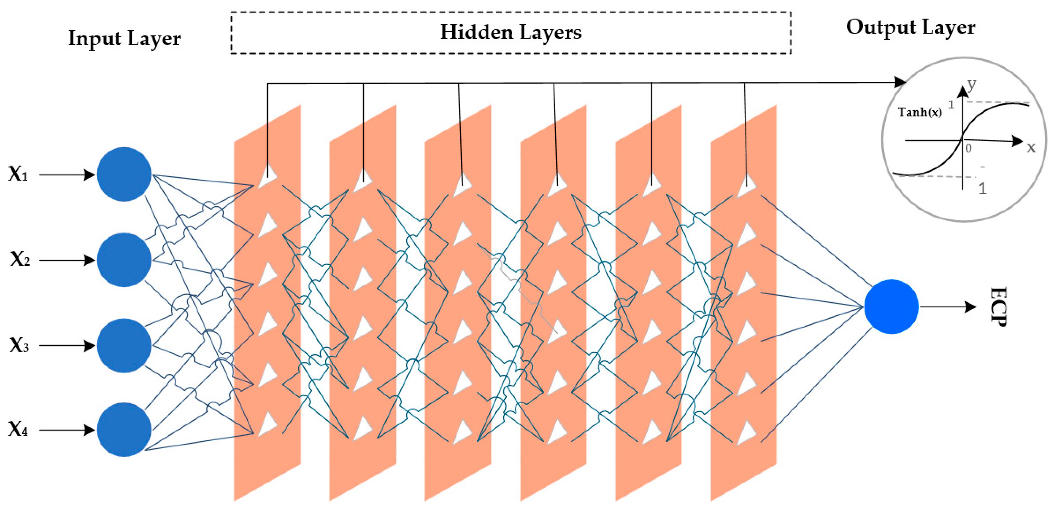
3.3.1. Deep Extreme Learning Machine (DELM)

The extreme learning machine (ELM) technique is a very famous technique and it has been used in different fields for energy consumption prediction. The conventional artificial neural network based algorithm requires more training samples, slower learning times, and may lead to the over-fitting of a learning model [40]. The idea of ELM was first specified by Reference [41]. The ELM is used widely in various areas for classification and regression purposes because an ELM learns very quickly and it is computationally efficient. The ELM model comprises the input layer, a single hidden layer, and an output layer. The structural model of an ELM is shown in Figure 6, where p represents input layer nodes, q represents hidden layer nodes, and r indicates output layer nodes.

Initially, take a sample of training $\left[A,B\right]=\left\{a_{k,}{b}_{k,}\right\}\left(i=1,2,\dots ,Z\right)$, and input feature $A=\left[a_{k1}{a}_{k2}{a}_{k3}\dots a_{kZ}\right]$ and a targeted matrix $B=\left[b_{l1}{b}_{l2}{b}_{l3}\dots b_{lZ}\right]$ consisted of the training samples, then A and B matrices can be represented as in Equations (3) and (4) respectively, where, a and b represent the dimension of the input matrix and the output matrix respectively. Next, the ELM arbitrarily adjusts the weights between the input layer and the hidden layer where $w_{kl}$ is the weight between the kth input layer node and lth hidden layer node as represented in Equation (5). Then, the ELM randomly fixes the weights between the hidden neurons and output layer neurons that can be represented by Equation (6), where ${\gamma }_{kl}$ is the weight between the input and hidden layer nodes.

$$A=\left[\begin{array}{c}{a}_{11}{a}_{12}...a_{1z}\\ a_{21}{a}_{22}...a_{2z}\\ a_{31}{a}_{32}...a_{3z}\\ \\ ⋮⋮⋮\\ a_{p1}{a}_{p2}...a_{pz}\\ \end{array}\right]$$

(3)

$$B=\left[\begin{array}{c}{b}_{11}{b}_{12}...b_{1z}\\ b_{21}{b}_{22}...b_{2z}\\ b_{31}{b}_{32}...b_{3z}\\ \\ ⋮⋮⋮\\ b_{r1}{b}_{r2}...b_{rz}\\ \end{array}\right]$$

(4)

$$\mathrm{w}=\left[\begin{array}{c}{w}_{11}{w}_{12}...w_{1p}\\ w_{21}{w}_{22}...w_{2p}\\ w_{31}{w}_{32}...w_{3p}\\ \\ ⋮⋮⋮\\ w_{i1}{w}_{i2}...w_{ip}\\ \end{array}\right]$$

(5)

$$\gamma =\left[\begin{array}{c}{\gamma }_{11}{\gamma }_{12}...{\gamma }_{1r}\\ {\gamma }_{21}{\gamma }_{22}...{\gamma }_{2r}\\ {\gamma }_{31}{\gamma }_{32}...{\gamma }_{3r}\\ \\ ⋮⋮⋮\\ {\gamma }_{p1}{\gamma }_{p2}...{\gamma }_{pr}\\ \end{array}\right]$$

(6)

Next, the biases of hidden layers nodes were randomly selected by the ELM, as in Equation (7). Further, the ELM selected a g(x) function, which was the activation function of the network. Consider Figure 4; the resultant matrix can be represented as in Equation (8). Respectively, the column vector of the resultant matrix, T, is represented in Equation (9).

$$B={\left[b_{1,}{b}_{2,}{b}_{3,\cdots ,}{b}_p\right]}^T$$

(7)

$$V={\left[v_1,v_{2,}{v}_3,\cdots ,v_Z\right]}_{r\times Z}$$

(8)

$$v_l=\left[\begin{array}{c}\begin{array}{c}\begin{array}{c}{v}_{1j}\\ v_{2j}\end{array}\\ t_{3j}\end{array}\\ ⋮\\ t_{rj}\end{array}\right]={\left[\begin{array}{c}\begin{array}{c}\begin{array}{c}{\displaystyle {{\displaystyle \sum }}_{l=1}^q}{\gamma }_{k1}g\left(w_k{a}_l+b_k\right)\\ {\displaystyle {{\displaystyle \sum }}_{l=1}^q}{\gamma }_{k2}g\left(w_k{a}_l+b_k\right)\end{array}\\ {\displaystyle {{\displaystyle \sum }}_{l=1}^q}{\gamma }_{k3}g\left(w_k{a}_l+b_k\right)\end{array}\\ ⋮\\ {\displaystyle {{\displaystyle \sum }}_{l=1}^q}{\gamma }_{kr}g\left(w_k{a}_l+b_k\right)\end{array}\right]}_{\left(l=1,2,3,...,Q\right)}$$

(9)

Next, by considering Equations (8) and (9), we can obtain Equation (10). The hidden layer output is expressed as H and the transposition of V is represented as $V^{\prime }$ and weight matrix values of γ [42,43] were computed using the least square method as given in Equation (11).

$$\mathrm{H}\gamma =V^{\prime }$$

(10)

$$\gamma ={\mathrm{H}}^{+}{V}^{\prime }$$

(11)

The regularization term γ has been used in order to make the network more generalized and more stable [44].

Deep learning is emerging and is the most popular topic for researchers nowadays. A network having at least four layers with input/output layers meets the requirement of a deep learning network. In a deep neural network, the neurons of each layer are trained on a different set of parameters using the prior layer’s output. It enables the deep learning networks (DLN) to handle extensive data sets. Deep learning has grasped the attention of many researchers because it is very efficient to solve real-world problems. In the proposed work, we have used the DELM to encapsulate the advantages of both ELM and deep learning. The configuration model of DELM consisted of one input layer having four neurons, six hidden layers where each hidden layer consisted of 10 neurons, and one output layer having one neuron is illustrated in Figure 7. The trial and error method has been used to select the number of nodes in the hidden layers due to the unavailability of any specific mechanism for specifying hidden layers neurons. The projected output of the second hidden layer can be achieved as:

$$H_1=V{\gamma }^{+}$$

(12)

where ${\gamma }^{+}$ represents the general inverse of matrix $\gamma$. Hence, the values of the hidden layer 2 can be simply achieved by means of Equation (11) and the activation function inverse.

$$g\left(W_{1}H+B_1\right)=H_1$$

(13)

In the Equation (13), the parameters $W_1,H,B_1,\mathrm{and}{H}_1$ represent the weight matrix of the first two hidden layers, the bias of the first hidden layer neurons, the estimated output of first hidden layer, and the estimated output of the second hidden layer respectively.

$$W_{HE}=g^{-1}\left(H_1\right)H_E^{+}$$

(14)

$H_E^{+}$ represents the inverse of $H_E$ and the activated function g(x) is used to compute Equation (5). So by specifying any proper activation function g(x), the desired result of the second hidden layer is updated as below:

$$H_2=g\left(W_{HE}{H}_E\right).$$

(15)

The update of the weighted Matrix $\gamma$ between hidden layer 2 and hidden layer 3, carried out as in Equation (16), where $H_2^{+}$ indicates the inverse of $H_2$. Therefore, the estimated result of the layer 3 is represented as in Equation (17).

$${\gamma }_{new}=H_2^{+}V$$

(16)

$$H_3=V{\gamma }_{new}^{+}$$

(17)

$V{\gamma }_{new}^{+}$ represents the inverse of the weight matrix ${\gamma }_{new}$. Then the DELM defines the matrix $W_{HE1}=\left[B_2,W_2\right]$. The output of the third layer can be achieved by using Equations (10) and 11).

$$H_3=g^{-1}\left(H_2{W}_2+B_2\right)=g\left(W_{HE1}{H}_{E1}\right)$$

(18)

$$W_{HE1}={\gamma }^{-1}(H_3)H_{E1}^{+}).$$

(19)

In Equation (18) the $H_2$ signifies the desired result and the hidden layer 2, the weight between the hidden layer 2 and the hidden layer 3 is represented by $W_2$, the hidden layer $B_2$ is the bias of the hidden layer 3 neurons. $H_{E1}^{+}$ represents the inverse of $H_{E1}$, and $g^{-1}\left(x\right)$ denotes the inverse of the activation function g(x). The logistic sigmoid function represented in Equation (20) has been adopted. The third hidden layer output is computed as in Equation (21).

$$g\left(x\right)=\frac{1}{1+e^{-x}}$$

(20)

$$H_3=g\left(W_{HE1}{H}_{E1}\right).$$

(21)

Finally, the resultant weighted matrix between the hidden layer 3 and the last layer output is computed as in Equation (22). The estimated result of the hidden layer 3 is represented as in Equation (23).

$${\gamma }_{new}=H_4^T{(\frac{1}{\lambda }+H_4^T{H}_4)}^{-1}V$$

(22)

$$H_4=V{\gamma }_{new}^{+}$$

(23)

$V{\gamma }_{new}^{+}$ represents the inverse of the weight matrix ${\gamma }_{new}$. Then the DELM defines the matrix $W_{HE2}=\left[B_3,W_3\right]$. The output of the fourth layer can be achieved by using Equations (15) and (24).

$$H_4=g^{-1}\left(H_3{W}_3+B_3\right)=g\left(W_{HE1}{H}_{E1}\right)$$

(24)

$$W_{HE2}={\gamma }^{-1}((H_4)H_{E2}^{+}).$$

(25)

In Equation (11), the $H_3$ denotes the desired output of the third hidden layer, the weight between the third hidden layer and the fourth hidden layer is represented by $W_3$, the hidden layer $B_3$ is the bias of the third hidden layer neurons. $H_{E1}^{+}$ represents the inverse of $H_{E1}$, and $g^{-1}\left(x\right)$ denotes the inverse of the activation function g(x). The logistic sigmoidal function has been adopted. The output of the third and fourth hidden layer is computed as Equation (26) below:

$$H_4=g\left(W_{HE2}{H}_{E2}\right)$$

(26)

Finally, the output weight matrix between the fourth layer and the output layer is computed as in Equation (27). The estimated result of the fifth layer can be denoted by Equation (28). The desired output of the DELM network is represented by Equation (29).

$${\gamma }_{new}=H_5^T{(\frac{1}{\lambda }+H_5^T{H}_5)}^{-1}V$$

(27)

$$H_5=V{\gamma }_{new}^{+}$$

(28)

$$f\left(x\right)=H_5{\beta }_{new.}$$

(29)

So far, we have discussed the calculation process of the four hidden layers of the DELM network. The cycle theory has been applied to demonstrate the calculation process of the DELM. The recalculation of Equations (18)–(22) can be done to get and record each hidden layer’s parameters and eventually the last result of DELM network. If increments occur in the hidden layers, the same computation procedure can be reused and executed similarly. In the proposed work we have applied a trial and error method [30,31] to determine the optimal neural network structure. Inputs to the DELM as shown in Figure 7 are hours of the day (X₁), days of the week (X₂), days of the month (X₃) and month (X₄) and the output is the energy consumption prediction (ECP).

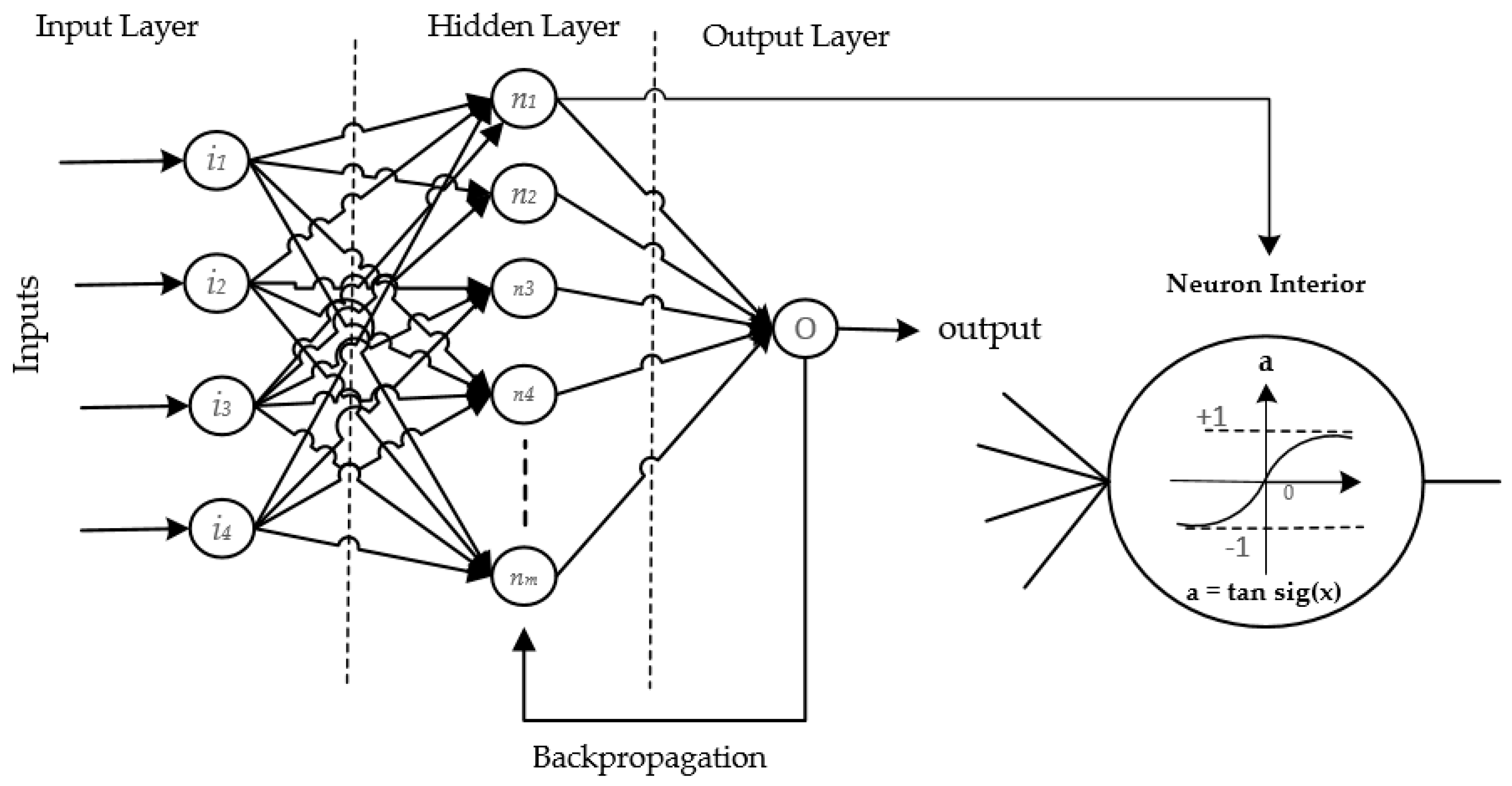
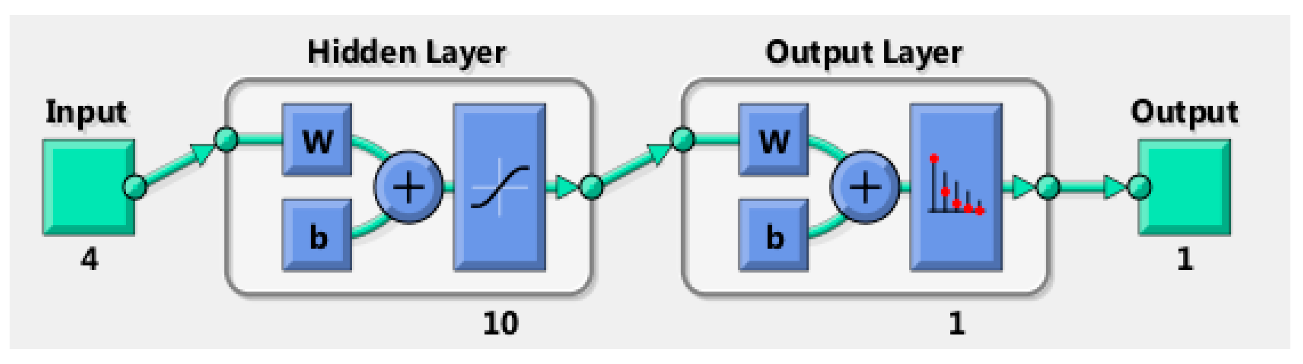
3.3.2. Artificial Neural Network (ANN)

ANNs are based on biological information processing and have been extensively used for energy consumption prediction in residential buildings. The ANNs have been commonly used because of their robust nonlinear mapping capability. The ANN might be reflected in a regression method, which signifies the sophisticated nonlinearity between independent and dependent variables [45]. In recent years, researchers have deployed ANN models for analyzing numerous types of prediction problems in a variety of circumstances. The ANN model used in the proposed work is the multilayer perceptron (MLPs). MLPs usually have three layers namely input, hidden, and the output consisting of input nodes, neurons, and synaptic connections. In MLPs backpropagation method is used to reduce the prediction residual sum of squares (RSS). The mathematical representation of RSS is given in the Equation (30).

$$\mathrm{RSS}={\displaystyle {{\displaystyle \sum }}_{i=1}^n}{(Y_i-\overline{Y_i})}^2$$

(30)

where $Y_i$ represents the ith targeted values in the training data and $\overline{Y_i}$ indicates the predicted values. The strength of the input signal is represented through synapse weights, and initially, these weights are initially allocated randomly. The sum of the product of each connection input value and synapse is computed and provided as input to each neuron in the hidden layer. Commonly three types of activation functions, namely linear, tan-sigmoid, and logarithmic sigmoid as represented in Equations (31)–(33) respectively are used in the hidden layer and output layer of MLP [30].

$$\mathsf{\chi }\left(\mathrm{x}\right)=\mathrm{linear}\left(\mathrm{x}\right)$$

(31)

$$\mathsf{\Phi }(\mathrm{x})=\frac{2}{\left(1+e^{-2x}\right)}-1$$

(32)

$$\mathsf{\psi }(\mathrm{x})=\frac{1}{\left(1+e^{-x}\right)}$$

(33)

The tan-sigmoid function is used as the activation function in the hidden layer. The best transfer function selection in the hidden is also somewhat trial and test method [46]. In the proposed work, we have tested five transfer functions, such as tan-sigmoid, linear, radial basis, symmetric, and saturating linear. In the output layer linear function has been used which is the most appropriate activation function for output neuron (s) of ANNs for regression problems. The structure diagram of the ANN used in the proposed approach is shown in Figure 8.

Different training algorithms, such as Levenburg Marquardt (LM), Bayesian regularization, scaled conjugate gradient and so forth [47] have been used for network training. The development of MLP with the number of pre-defined hyper-parameters disturbs the ability of fitness of the model. The selection of the number of neurons in the hidden layer is a somewhat trial and test method [30].

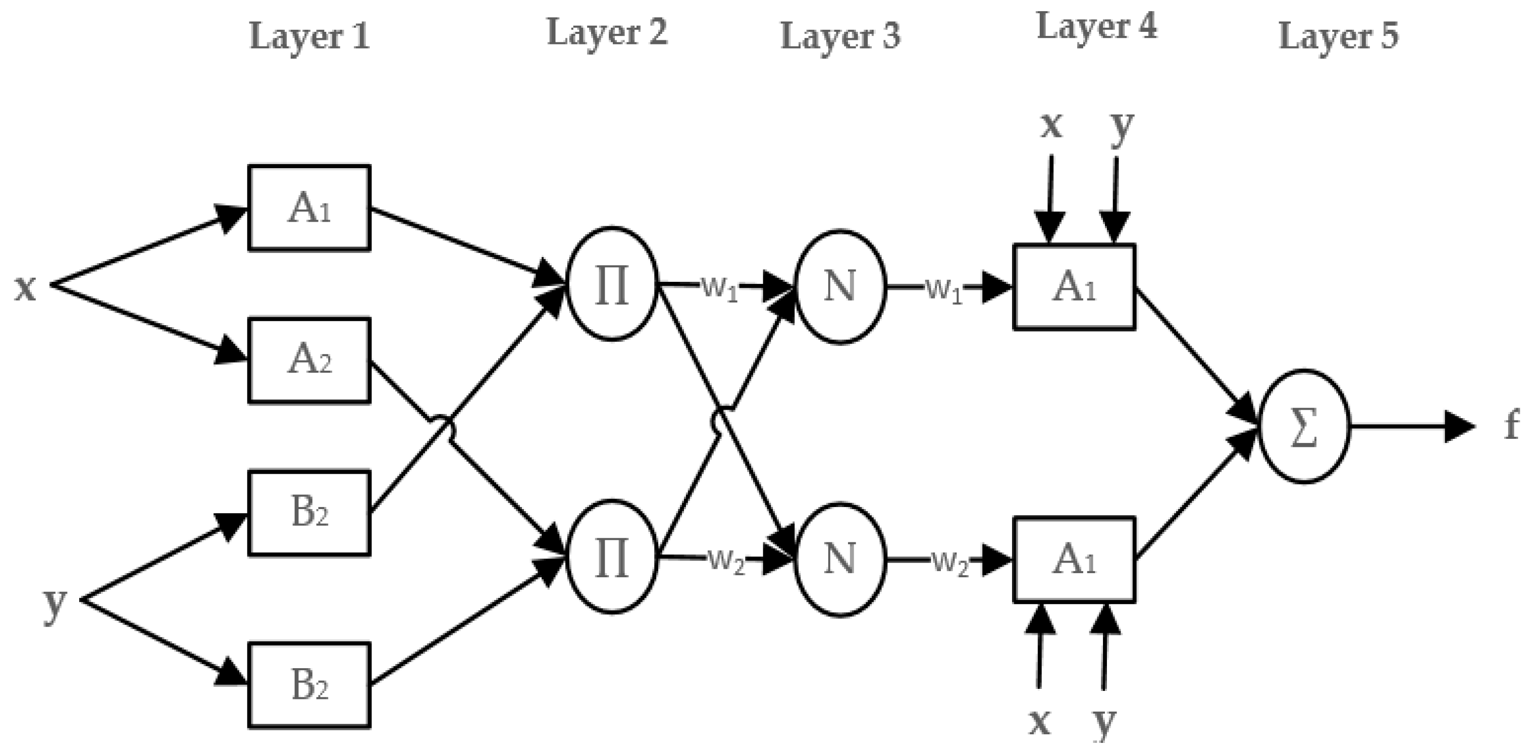
3.3.3. Adaptive Neuro-Fuzzy Inference System (ANFIS)

ANFIS uses a feed-forward network having multiple layers which use NN algorithms for learning and fuzzy reasoning for mapping the input space to output space. ANFIS is used extensively in various areas for predictions [48,49,50]. ANFIS is a fuzzy inference system (FIS), and its implementation is carried out in the adaptive neural framework. The structure of ANFIS is shown in Figure 9 (2 inputs, and one output) for the first order Sugeno fuzzy logic model. In this structure, for each input, two membership functions have been defined.

The adaptive neuro-fuzzy system consisted of five different layers, each of them is explained below in detail such as layer 1 nodes are adaptive and produce inputs degree of membership functions (MFs). Layer 2 nodes are fixed, and these nodes do simple multiplication. Layer 3 nodes are also fixed, and the role of these nodes in the network is normalization. Layer 4 nodes are adaptive whose output is a simple multiplication of normalized firing strength and first-order Sugeno model. The factors of this layer are named as consequent factors. Layer 5 has a single permanent node where the calculation of all incoming is carried out.

The supervised learning is used to train the network. Hence, the purpose is to train the adaptive network for known functions approximation supplied by training data and then finds the exact value of the mentioned parameters. There is no hard and fast rule to determine a suitable number of membership functions for a variable in ANFIS. In the proposed work, we have applied the trial and error mechanism to determine the effective number of MFs for each variable. Similarly, there are many types of membership functions, such as triangular, trapezoidal, and so forth [49]. In the proposed work, we have considered the bell-shaped membership functions as illustrated in Equations (34) and (35).

$${\mathsf{\mu }}_{{\mathrm{X}}_{\mathrm{i}}}\left(\mathrm{a}\right)=\frac{1}{1+{\left(\frac{\mathrm{a}-{\mathrm{c}}_{\mathrm{i}}}{{\mathrm{a}}_{\mathrm{i}}}\right)}^{2{\mathrm{x}}_{\mathrm{i}}}},\mathrm{i},1,2,$$

(34)

$${\mathsf{\mu }}_{{\mathrm{Y}}_{\mathrm{i}}}\left(\mathrm{b}\right)=\frac{1}{1+{\left(\frac{\mathrm{b}-{\mathrm{c}}_{\mathrm{i}}}{{\mathrm{a}}_{\mathrm{i}}}\right)}^{2{\mathrm{x}}_{\mathrm{j}}}},\mathrm{j},1,2,$$

(35)

The bell-shaped membership functions are the most common and effective MFs used in the ANFIS for prediction purposes [51].

3.4. Performance Evaluation Layer

Several criteria are used for performance computation of different prediction algorithms. In the performance evaluation layer of the proposed model, MAE, RMSE, and MAPE performance indices have been used to compare the target values and the actual values. The MSE is a measure that used for the minimization of the error distribution. The RMSE measures the error between the predicted power and the targeted power, and the MAPE is a measure which evaluates the prediction difference as a percentage of the targeted power. The RMSE, MAE, and MAPE performance can be computed in Equations (36)–(38) respectively as:

$$\mathrm{RMSE}=\sqrt{\frac{1}{\mathrm{N}}{\displaystyle {{\displaystyle \sum }}_{\mathrm{k}=0}^{\mathrm{n}}}{({\mathrm{T}}_{\mathrm{i}}-{\mathrm{P}}_{\mathrm{i}})}^2}$$

(36)

$$\mathrm{MAE}=\frac{1}{\mathrm{N}}{\displaystyle {{\displaystyle \sum }}_{\mathrm{i}=1}^{\mathrm{n}}}\left|{\mathrm{T}}_{\mathrm{i}}-{\mathrm{P}}_{\mathrm{i}}\right|$$

(37)

$$\mathrm{MAPE}=\frac{1}{\mathrm{N}}{\displaystyle {{\displaystyle \sum }}_{\mathrm{i}=1}^{\mathrm{n}}}\frac{\left|{\mathrm{T}}_{\mathrm{i}}-{\mathrm{P}}_{\mathrm{i}}\right|}{{\mathrm{T}}_{\mathrm{i}}}\text{×}100$$

(38)

where N indicates the entire values, T represents the target value, and P indicates the predicted value. These metrics provide a single value to measure the accuracy of the outcomes of different algorithms. These statistical measurements have been used in previous studies to analyze energy consumption prediction models [34].

4. Experimental Results Based on Prediction Algorithms

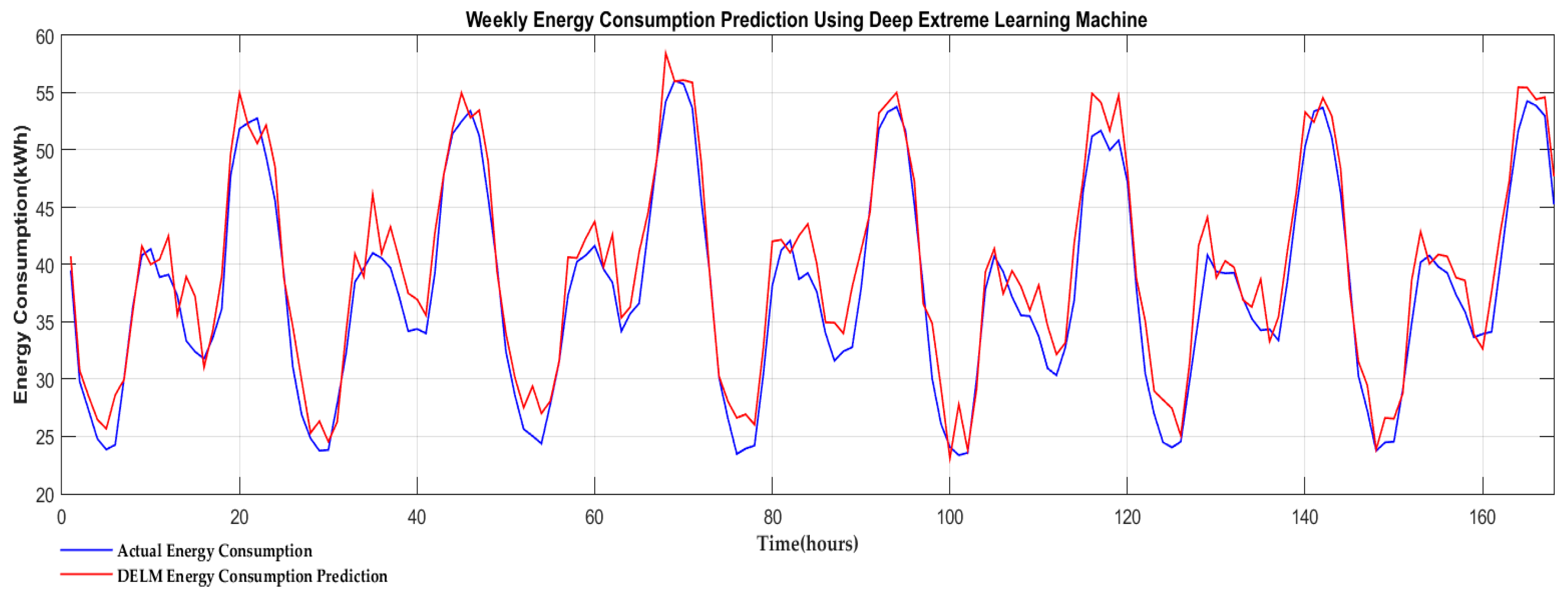
4.1. Model Validation of DELM

To validate the model and analyze the experiments we have used, the actual data collected by using different meters fixed in the designated multi-storied residential buildings. The data is collected for a single year, i.e., 1 January 2010 to 31 December 2010. The size of complete input data is equal to 365 days × 24 h per day = 8760. The installation of smart meters at each floor sub-distribution switchboard has been carried out, and these meters are in connection with the central server. The energy consumption for each hour is recorded for a year, and the unit used for measurement is Kilowatt hour (kWh). The information contained by data-set is floor-wise hourly energy consumption. Example view for two days hourly collected data is illustrated in Figure 10 for anonymous building-04 having 33 floors.

We have used four important parameters, hours of the day (X₁), days of the week (X₂), days of the month (X₃) and month (X₄) as input to machine learning algorithms used in the proposed work. Further, to prevent overfitting, we used the k-fold cross-validation. It is a popular method because it is simple to understand and generally results in a less biased or less optimistic estimate of the model skill than other methods, such as a simple train/test split [52]. For one-week energy consumption prediction the data is divided into 52 folds of approximately equal size. The first fold is treated as a validation set, and the method is fit on the remaining folds. In the proposed work, we have carried out energy consumption prediction for one-week and one-month. Hence, for a one-week energy consumption prediction, one year hourly data is divided into 52 folds. In testing data set we have used the one-week (7 days × 24 h = 168) data for testing and the remaining data (358 days × 24 h = 8592) to train the models for one week energy consumption prediction. We have swapped the results achieved for one-week energy consumption prediction, and next to the training and testing data and randomly selected another data set (one week) for testing and the remaining for training.

This process continues until 52 iterations. Similar, for one-month energy consumption prediction the data have been divided into 12 (k) sets with approximately equal size. We have used the one-month (January) (31 days × 24 h = 744 h) data for testing and the remaining 11 months data (8016 h) for training. Next, we have selected another month (February) data (28 days × 24 h = 672 h) for testing and the remaining 11 months hourly data (8088 h) for training. The processes continue until the 12th month (December) hourly data (31 days × 24 h = 744 h) get selected for testing and the remaining (11 months data) (31 days × 24 h = 744 h) for training. Finally, the average of the testing results was determined.

The optimum network configuration depends on the number of hidden layers, a number of neurons in the hidden layer (s), and the type of activation function. We have applied trial and error method to achieve the optimum structure [46]. After applying trial and error method, we achieved the well-suited configuration model consisted of 6 hidden layers and 20 neurons in each hidden layer for the proposed DELM approach. The sigmoid activation function is used as activation function because it is the most popular activation function and numerously used from the last couple of years [51]. We have also tried different iteration numbers from 1000 to 3000 with 100 increments and set iteration number as 2000. Now by using the best-suited configuration model the one-week and one-month hourly energy consumption resulted are recorded as shown in Figure 11 and Figure 12 respectively.

In this work, we have used ANN and ANFIS models for comparison with ANN and DELM. The reason behind the selection of ANFIS was its ability to seek for useful features and development of the prediction model. The ANNs is also a very famous technique and it is used for energy consumption purposes.

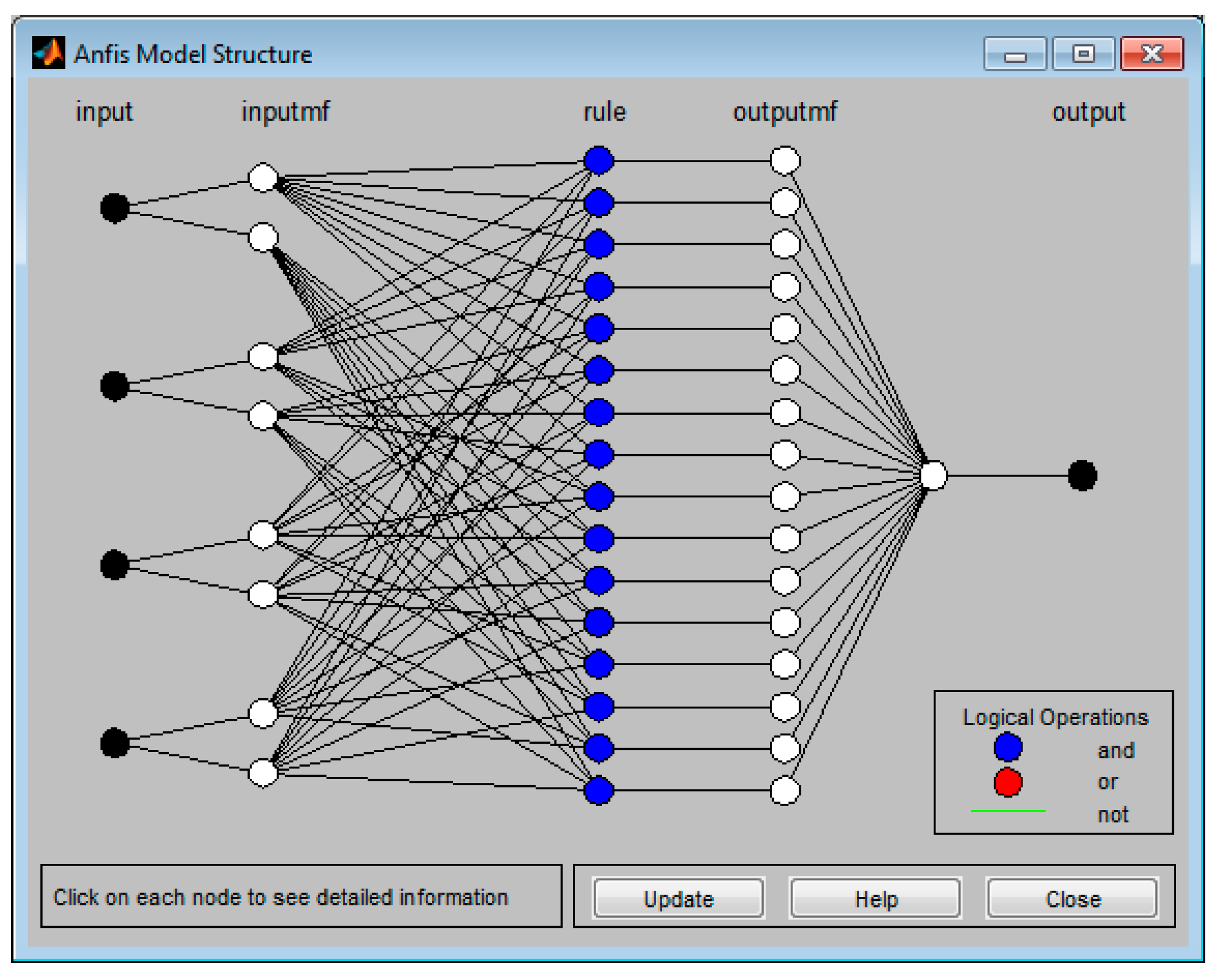
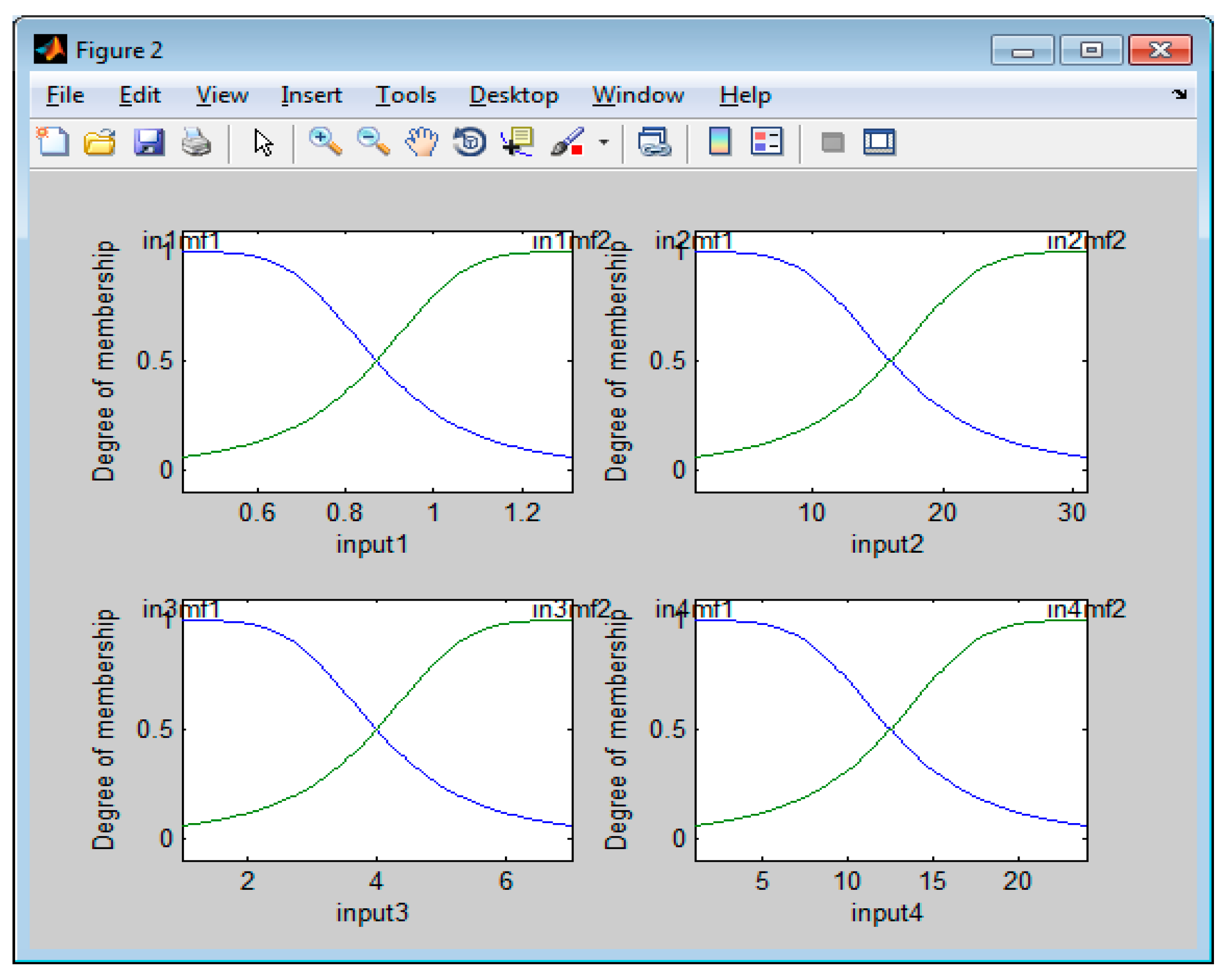
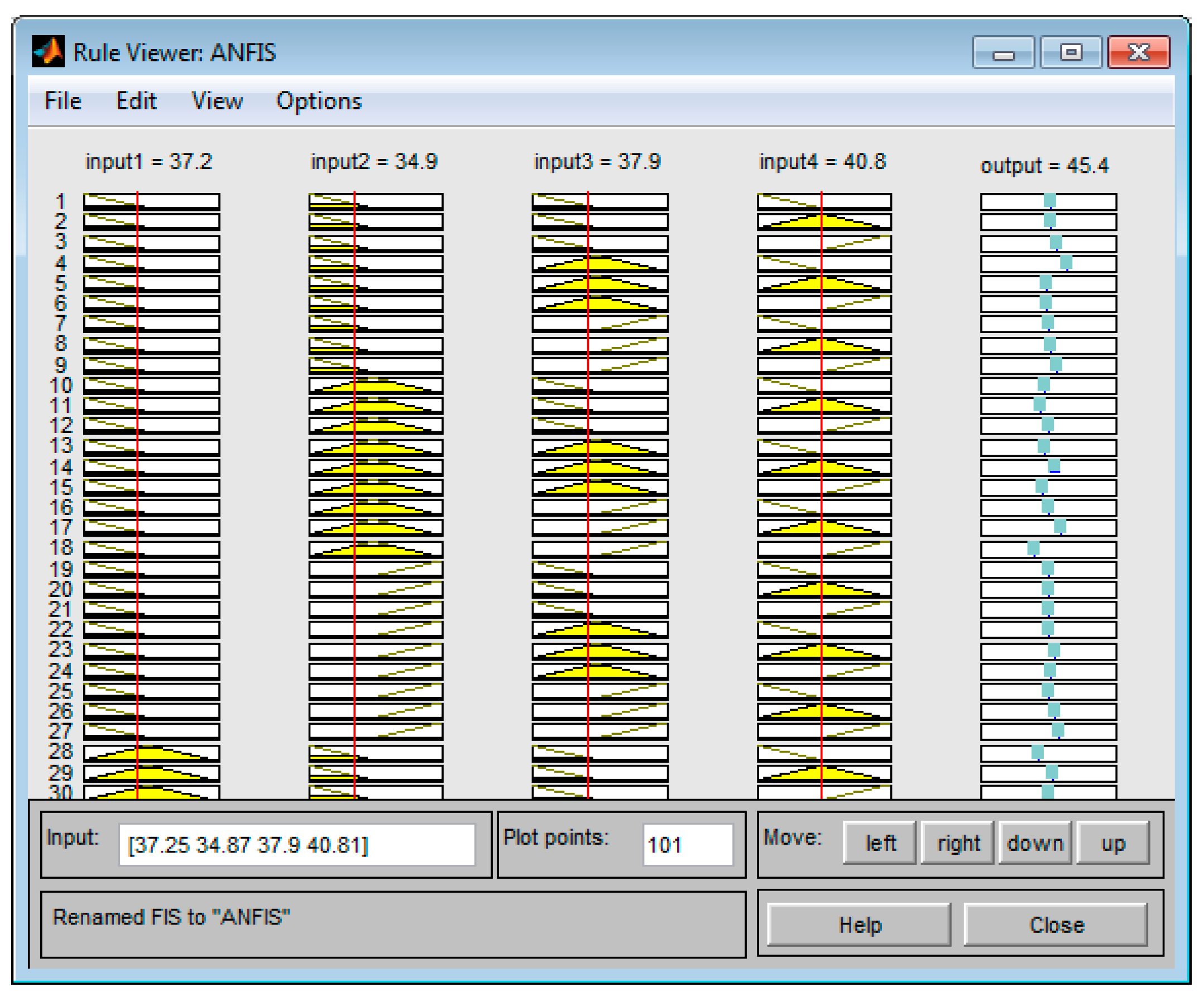
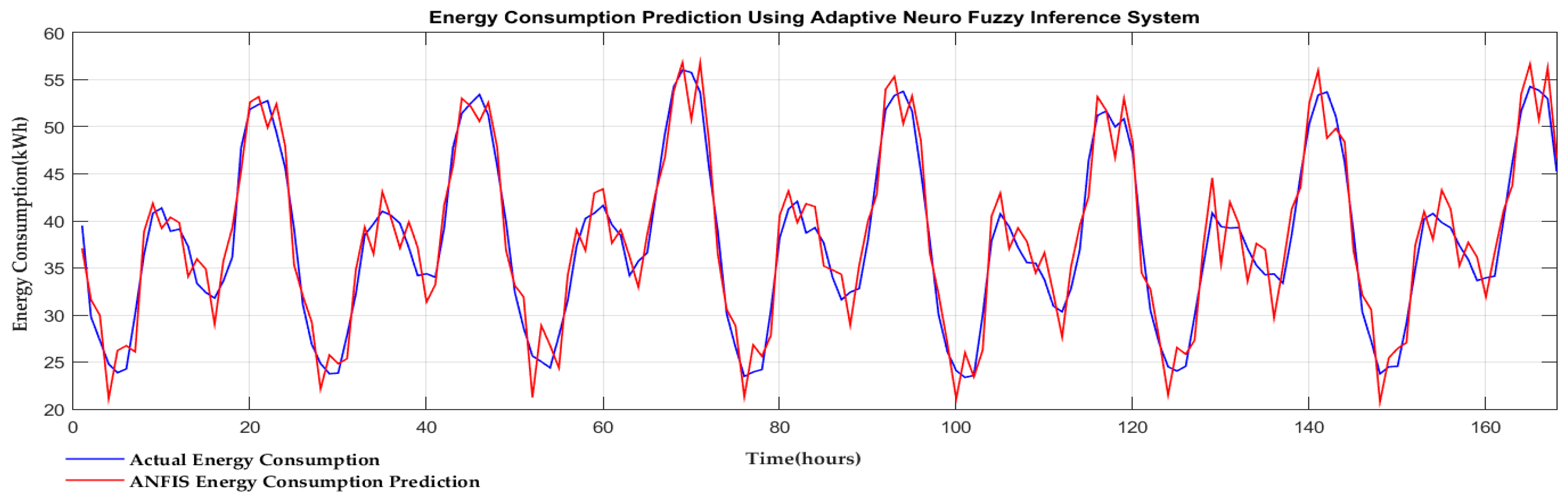
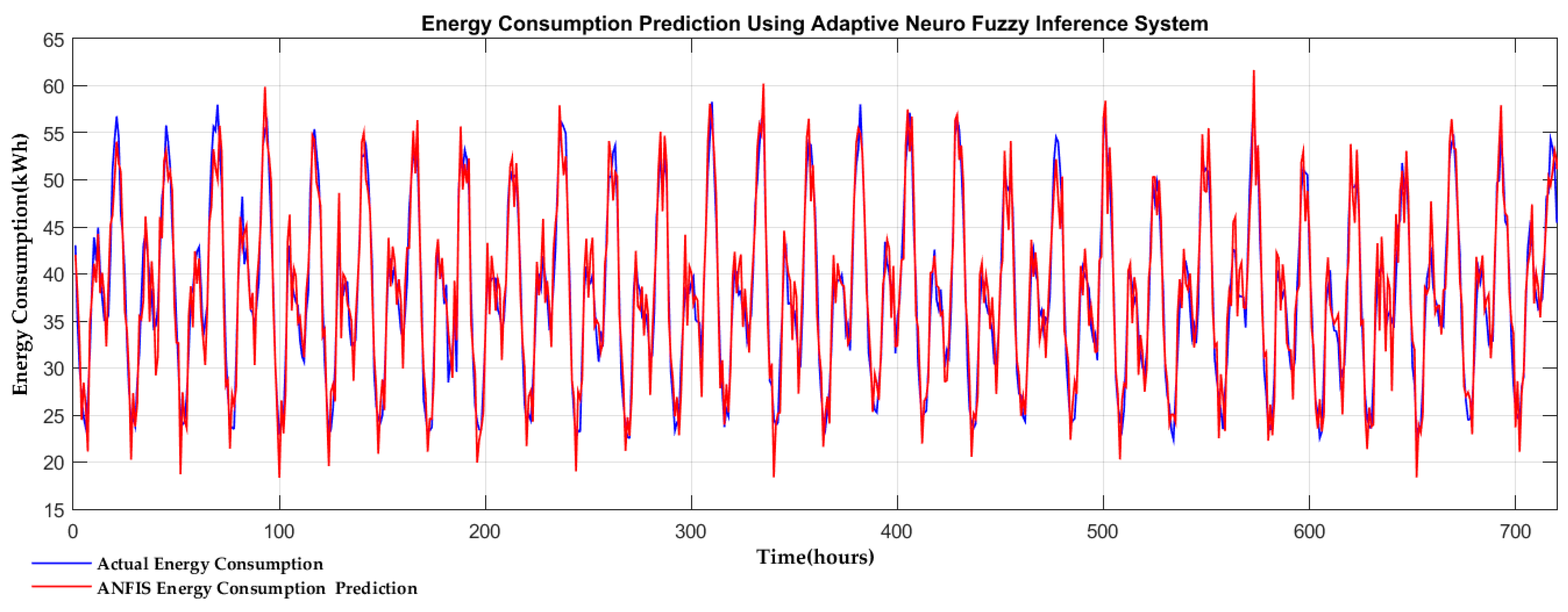
4.2. Model Validation of ANFIS

The structure diagram of the ANFIS for the proposed work is shown in Figure 13 [53]. We have used a trial and error approach for the type and number of membership functions selection in the proposed work. For each variable, we have considered two generalized bell-shaped MFs as shown in Figure 14. Total 16 rules were specified; the rule viewer is shown in Figure 15.

The output predicted results for one-week and one-month energy consumption is shown in Figure 16 and Figure 17 respectively.

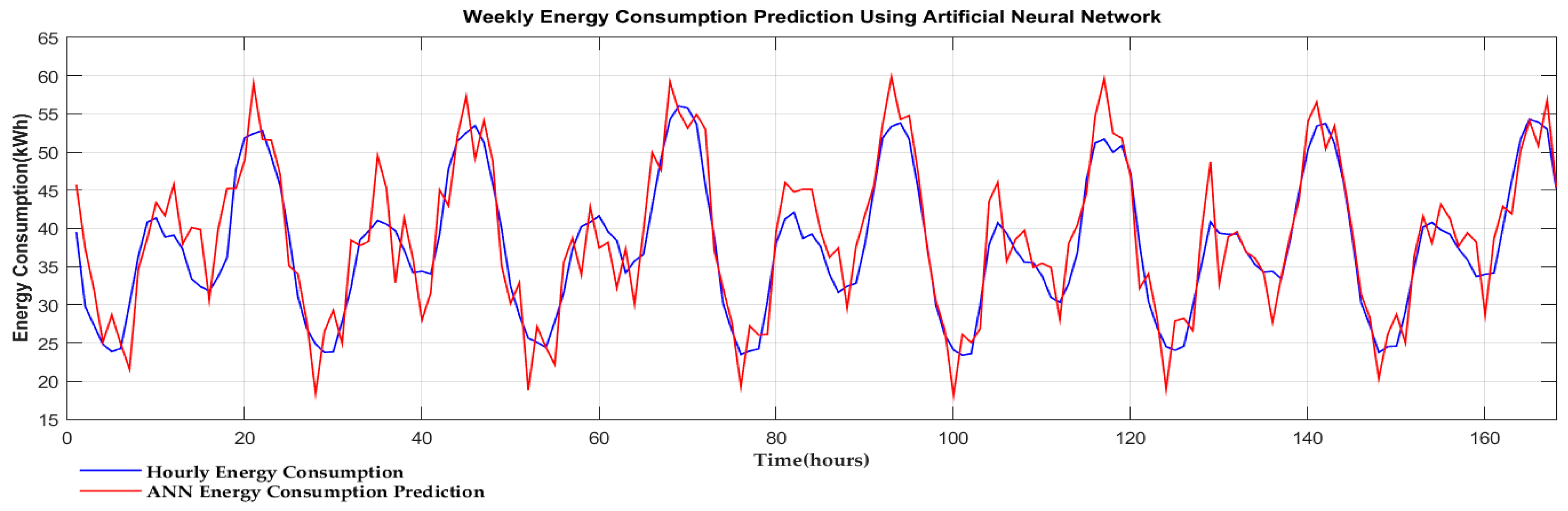
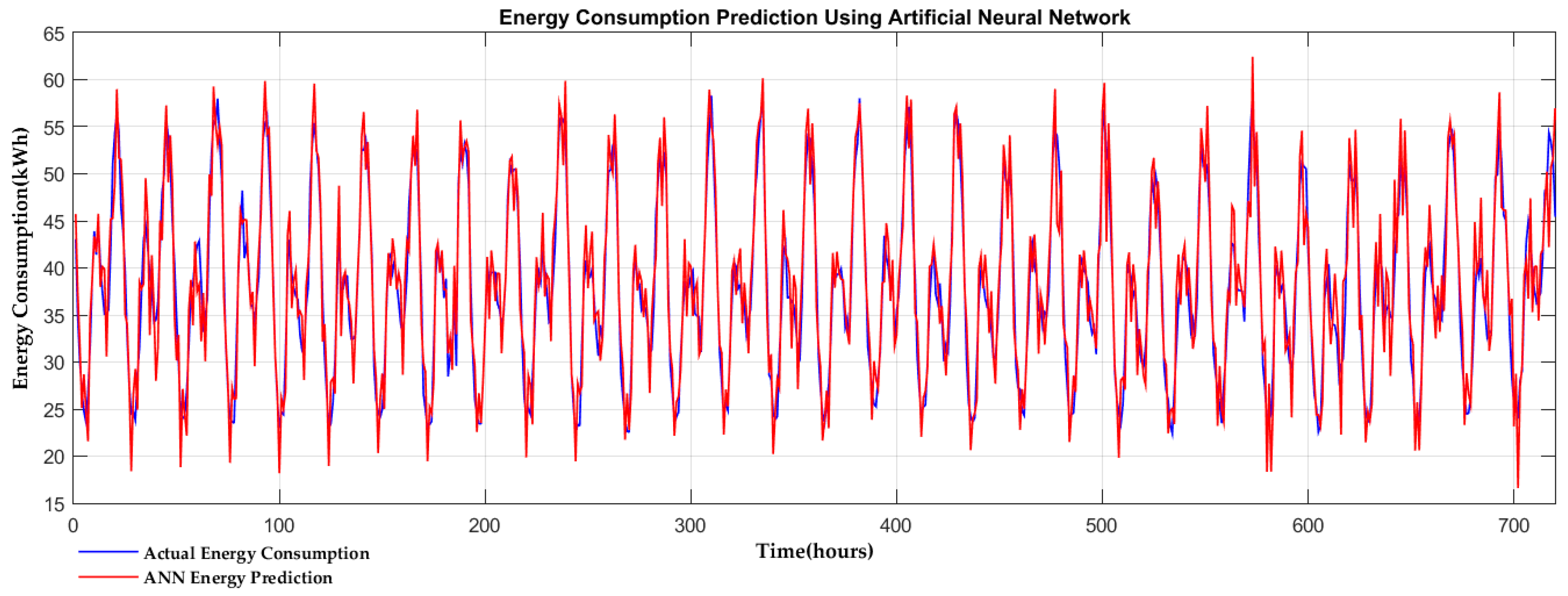
4.3. Model Validation of ANN

In the proposed work for achieving the best ANN prediction model, we tried different hidden layer activation functions, different training functions, and output layer transfer functions instead of the sensitivity of input parameters. All the network models have four neurons in input layer, a single neuron in output layer and for hidden layer, we have tried some neurons in the hidden layer started from 5 to 30 with five increments to find best combination input layer, hidden layer, and output layer neurons Trial and error method has been applied to determine the number of neurons in hidden layers [30]. We have considered the model as shown in Figure 18 because it provides the least MSE values with tan-sigmoid (x) function in the hidden layer, linear function in the output layer and the Levenberg-Marquardt algorithm for training.

The recorded energy consumption prediction results for one-week and one-month have been shown in Figure 19 and Figure 20 respectively.

5. Discussion and Comparative Results Analysis

In the proposed work, we have applied the deep extreme learning algorithm along with ANN and ANFIS on real data collected for one year to predict energy consumption in buildings for one-week and one-month. The data have been pre-processed to remove abnormalities from the data and make the data smooth and error free. In the DELM different number of hidden layers, hidden neurons, different combinations of activation functions have been tried to find the best configuration model for energy consumption prediction. For a fair comparison, we also apply trial and error approach for ANN to find the best configuration model. Hence, we have tried different numbers of neurons in hidden layers, different types of activation functions, and different numbers of neurons in the hidden layer. Similarly, we also tested different types of membership functions and different numbers of membership functions to achieve the suitable structure of ANFIS for energy consumption prediction.

In this work, we have applied the proposed DELM for two different periods of time energy consumption prediction along with optimized ANN, and ANFIS approaches to test the efficiency of these algorithms properly. For one-week energy consumption prediction the data into training set would be more significant as compared to one-month energy consumption prediction. Hence to properly evaluate the performance of prediction algorithms both short-term and long-term energy consumption prediction have been carried output.

We have used different statistical measures to measure the performance of the proposed DELM algorithm along with counterpart algorithms. In

Table 1. Performance evaluation of deep extreme learning machine (DELM), adaptive neuro-fuzzy inference system (ANFIS) and artificial neural network (ANN) for one-week energy consumption prediction.

Statistical Measures	MAE	MAPE	RMSE
DELM	2.0008	5.7077	2.2451
ANFIS	2.2679	6.3884	2.4636
ANN	2.3918	6.7097	2.6030

and

Table 2. Performance evaluation of DELM, ANFIS and ANN for one-month energy consumption prediction.

Statistical Measures	MAE	MAPE	RMSE
DELM	2.3347	6.5464	2.6864
ANFIS	2.6433	7.3798	3.1712
ANN	2.5437	7.4562	3.2400

the MAE, RMSE and MAPE values of DELM, ANN and ANFIS for one-week and one-month energy consumption prediction have been recorded. As in the proposed work, we have computed the one-month and one-week energy consumption prediction using machine learning algorithms. Hence the average of statistical measures values for both periods for the used prediction algorithms have been computed in

Table 3. Average values of statistical measures for one-week and one-month energy consumption prediction results of DELM, ANFIS, and ANN.

Statistical Measures	MAE	MAPE	RMSE
DELM	2.1677	6.1271	2.4657
ANFIS	2.4556	6.8841	2.8174
ANN	2.4317	7.0830	4.8561

. These statistical measures values indicate that the DELM performance is far better than the other counterpart algorithms. The performance of ANFIS is better as compared to the ANN.

The statistical measures values indicate that the performance of the proposed DELM is far better than the ANN and ANFIS for short-term (one-week) as well as on long-term (one-month) hourly energy consumption prediction. So, the proposed DELM is the best choice for the energy consumption prediction for both short and long terms energy consumption prediction.

6. Conclusions and Future Work

Modelling of energy consumption prediction in residential buildings is a challenging task, because of randomness and noisy disturbance. To obtain better prediction accuracy, in this paper, we have proposed a model for energy consumption prediction in residential buildings. The proposed model comprised of four stages, namely data acquisition layer, a preprocessing layer, the prediction layer, and performance evaluation layer. In data acquisition layer the data was collected through smart meters in a designated building to validate the model and analyze the results. In the preprocessing layer, some pre-processing operations have been carried out on the data to remove abnormalities from the data. In the second stage, we have proposed deep extreme learning machine and applied to the pre-processed data for one-week and one-month energy consumption prediction in residential buildings. The purpose of using different machine learning algorithms on collected data was to obtain better results in term of accuracy for practical applications. For the optimal structure of DELM different parameters various number of hidden layers, different numbers of neurons in the hidden layer and different activation functions have been tuned to get the optimized structure of DELM. We have also applied other well-known machine learning algorithms, such as ANN, and ANFIS one the same data for comparison with proposed DELM. We have used different statistical measures for performance measurements of these machine learning algorithms. These statistical measures values indicate that the performance of proposed DELM is far better as compared to other counterpart algorithms. These initial results give us confidence, and we are currently exploring various alternatives and collecting data to extend this work in directions above.

References

1. Fayaz, M.; Kim, D. Energy Consumption Optimization and user comfort management in residential buildings using a bat algorithm and fuzzy logic. Energies 2018, 11, 161. [Google Scholar] [CrossRef]
2. Selin, R. The Outlook for Energy: A View to 2040; ExxonMobil: Irving, TX, USA, 2013. [Google Scholar]
3. Sieminski, A. International Energy Outlook; Energy Information Administration: Washington, DC, USA, 2014. [Google Scholar]
4. Mitchell, B.M.; Ross, J.W.; Park, R.E. A Short Guide to Electric Utility Load Forecasting; Rand Corporation: Santa Monica, CA, USA, 1986. [Google Scholar]
5. Parez-Lombard, L.; Ortiz, J.; Pout, C. A review on buildings energy consumption information. Energy Build. 2008, 40, 394–398. [Google Scholar] [CrossRef]
6. Zhao, H.-X.; Magoulès, F. A review on the prediction of building energy consumption. Renew. Sustain. Energy Rev. 2012, 16, 3586–3592. [Google Scholar] [CrossRef]
7. Fumo, N. A review on the basics of building energy estimation. Renew. Sustain. Energy Rev. 2014, 31, 53–60. [Google Scholar] [CrossRef]
8. Ahmad, A.; Hassan, M.; Abdullah, M.; Rahman, H.; Hussin, F.; Abdullah, H.; Saidur, R. A review on applications of ANN and SVM for building electrical energy consumption forecasting. Renew. Sustain. Energy Rev. 2014, 33, 102–109. [Google Scholar] [CrossRef]
9. Kim, S.; Kim, S. A multi-criteria approach toward discovering killer iot application in Korea. Technol. Forecast. Soc. Change 2016, 102, 143–155. [Google Scholar] [CrossRef]
10. Malik, S.; Kim, D. Prediction-learning algorithm for efficient energy consumption in smart buildings based on particle regeneration and velocity boost in particle swarm optimization neural networks. Energies 2018, 11, 1289. [Google Scholar] [CrossRef]
11. Khosravani, H.R.; Castilla, M.D.M.; Berenguel, M.; Ruano, A.E.; Ferreira, P.M. A comparison of energy consumption prediction models based on neural networks of a bioclimatic building. Energies 2016, 9, 57. [Google Scholar] [CrossRef]
12. Kalogirou, S.A. Artificial neural networks in energy applications in buildings. Int. J. Low-Carbon Technol. 2006, 1, 201–216. [Google Scholar] [CrossRef]
13. Kampouropoulos, K.; Cárdenas, J.J.; Giacometto, F.; Romeral, L. An energy prediction method using adaptive neuro-fuzzy inference system and genetic algorithms. In Proceedings of the 2013 IEEE International Symposium on Industrial Eleactronics, Taipei, Taiwan, 28–31 May 2013. [Google Scholar]
14. Ullah, I.; Ahmad, R.; Kim, D. A prediction mechanism of energy consumption in residential buildings using hidden markov model. Energies 2018, 11, 358. [Google Scholar] [CrossRef]
15. Huang, G.B.; Zhu, Q.Y.; Siew, C.K. Extreme learning machine: Theory and applications. Neurocomputing 2006, 70, 489–501. [Google Scholar] [CrossRef] [Green Version]
16. Fan, C.; Xiao, F.; Zhao, Y. A short-term building cooling load prediction method using deep learning algorithms. Appl. Energy 2017, 195, 222–233. [Google Scholar] [CrossRef]
17. Schmidhuber, J. Deep learning in neural networks: An overview. Neural Netw. 2015, 61, 85–117. [Google Scholar] [CrossRef] [PubMed] [Green Version]
18. Li, L.; Lv, Y.; Wang, F.Y. Traffic signal timing via deep reinforcement learning. IEEE/CAA J. Autom. Sin. 2016, 3, 247–254. [Google Scholar]
19. Lv, Y.; Duan, Y.; Kang, W.; Li, Z.; Wang, F.Y. Traffic flow prediction with big data: A deep learning approach. IEEE Trans. Intell. Transp. Syst. 2015, 16, 865–873. [Google Scholar] [CrossRef]
20. Qiu, X.; Zhang, L.; Ren, Y.; Suganthan, P.N.; Amaratunga, G. Ensemble deep learning for regression and time series forecasting. In Proceedings of the 2014 IEEE Symposium on Computational Intelligence in Ensemble Learning (CIEL), Orlando, FL, USA, 9–12 December 2014; pp. 21–26. [Google Scholar] [CrossRef]
21. Kalogirou, S.; Neocleous, C.; Schizas, C. Building heating load estimation using artificial neural networks. In Proceedings of the Clima 2000 Conference, Brussels, Belgium, 30 August–2 September 1997. [Google Scholar]
22. Olofsson, T.; Andersson, S.; Östin, R. A method for predicting the annual building heating demand based on limited performance data. Energy Build. 1998, 28, 101–108. [Google Scholar] [CrossRef]
23. Yokoyama, R.; Wakui, T.; Satake, R. Prediction of energy demands using neural network with model identification by global optimization. Energy Convers. Manag. 2009, 50, 319–327. [Google Scholar] [CrossRef]
24. Kreider, J.; Claridge, D.; Curtiss, P.; Dodier, R.; Haberl, J.; Krarti, M. Building energy use prediction and system identification using recurrent neural networks. J. Sol. Energy Eng. 1995, 117, 161–166. [Google Scholar] [CrossRef]
25. Ben-Nakhi, A.E.; Mahmoud, M.A. Cooling load prediction for buildings using general regression neural networks. Energy Convers. Manag. 2004, 45, 2127–2141. [Google Scholar] [CrossRef]
26. Carpinteiro, O.A.; Reis, A.J.; da Silva, A.P. A hierarchical neural model in short-term load forecasting. Appl. Soft Comput. 2004, 4, 405–412. [Google Scholar] [CrossRef]
27. Gross, G.; Galiana, F.D. Short-term load forecasting. Proc. IEEE 1987, 75, 1558–1573. [Google Scholar] [CrossRef]
28. Irisarri, G.; Widergren, S.; Yehsakul, P. On-line load forecasting for energy control center application. IEEE Trans. Power App. Syst. 1982, 71–78. [Google Scholar] [CrossRef]
29. Ali, S.; Kim, D.-H. Effective and comfortable power control model using kalman filter for building energy management. Wirel. Pers. Commun. 2013, 73, 1439–1453. [Google Scholar] [CrossRef]
30. Wahid, F.; Kim, D.H. Short-term energy consumption prediction in korean residential buildings using optimized multi-layer perceptron. Kuwait J. Sci. 2017, 44, 67–77. [Google Scholar]
31. Wahid, F.; Kim, D.H. A prediction approach for demand analysis of energy consumption using K-nearest neighbor in residential buildings. Int. J. Smart Home 2016, 10, 97–108. [Google Scholar] [CrossRef]
32. Arghira, N.; Hawarah, L.; Ploix, S.; Jacomino, M. Prediction of appliances energy use in smart homes. Energy 2012, 48, 128–134. [Google Scholar] [CrossRef]
33. Li, K.; Su, H.; Chu, J. Forecasting building energy consumption using neural networks and hybrid neuro-fuzzy system: A comparative study. Energy Build. 2011, 43, 2893–2899. [Google Scholar] [CrossRef]
34. Kassa, Y.; Zhang, J.; Zheng, D.; Wei, D. Short term wind power prediction using ANFIS. In Proceedings of the 2016 IEEE International Conference on Power and Renewable Energy (ICPRE), Shanghai, China, 21–23 October 2016; pp. 388–393. [Google Scholar]
35. Ekici, B.B.; Teoman Aksoy, U. Prediction of building energy needs in early stage of design by using ANFIS. Expert Syst. Appl. 2011, 38, 5352–5358. [Google Scholar] [CrossRef]
36. Collobert, R.; Weston, J. A unified architecture for natural language processing: Deep neural networks with multitask learning. In Proceedings of the 25th International Conference on Machine Learning, Helsinki, Finland, 5–9 July 2008; pp. 160–167. [Google Scholar]
37. Hinton, G.E.; Salakhutdinov, R.R. Reducing the dimensionality of data with neural networks. Science 2006, 313, 504–507. [Google Scholar] [CrossRef] [PubMed]
38. Nau, R. Forecasting with Moving Averages. Fuqua School of Business, Duke University, 2014. Available online: https://people.duke.edu/~rnau/Notes_on_forecasting_with_moving_averages--Robert_Nau.pdf (accessed on 24 June 2018).
39. Niu, D.; Wang, H.; Chen, H.; Liang, Y. The general regression neural network based on the fruit fly optimization algorithm and the data inconsistency rate for transmission line icing prediction. Energies 2017, 10, 66. [Google Scholar] [CrossRef]
40. Cheng, J.; Duan, Z.; Xiong, Y. QAPSO-BP algorithm and its application in vibration fault diagnosis for a hydroelectric generating unit. Shock Vib. 2015, 34, 177–181. [Google Scholar]
41. Huang, G.-B.; Wang, D.H.; Lan, Y. Extreme learning machines: A survey. Int. J. Mach. Learn. Cybern. 2011, 2, 107–122. [Google Scholar] [CrossRef]
42. Wang, S.; Chen, H.; Yan, W.; Chen, Y.; Fu, X. Face recognition and micro-expression recognition based on discriminant tensor subspace analysis plus extreme learning machine. Neural Process. Lett. 2014, 39, 25–43. [Google Scholar] [CrossRef]
43. Huang, G. An insight into extreme learning machines: Random neurons, random features and kernels. Cogn. Comput. 2014, 6, 376–390. [Google Scholar] [CrossRef]
44. Wei, J.; Liu, H.; Yan, G.; Sun, F. Robotic grasping recognition using multi-modal deep extreme learning machine. Multidim. Syst. Signal Process. 2017, 28, 817–833. [Google Scholar] [CrossRef]
45. Geem, Z.W. Parameter estimation for the nonlinear muskingum model using the bfgs technique. J. Irrig. Drain. Eng. 2006, 132, 474–478. [Google Scholar] [CrossRef]
46. Shine, P.; Murphy, M.; Upton, J.; Scully, T. Machine-learning algorithms for predicting on-farm direct water and electricity consumption on pasture based dairy farms. Comput. Electron. Agric. 2018, 150, 74–87. [Google Scholar] [CrossRef]
47. Chau, K.W. Particle swarm optimization training algorithm for ANNs in stage prediction of Shing Mun River. J. Hydrol. 2006, 329, 363–367. [Google Scholar] [CrossRef] [Green Version]
48. Lo, S.-P. An adaptive-network based fuzzy inference system for prediction of workpiece surface roughness in end milling. J. Mater. Process. Technol. 2003, 142, 665–675. [Google Scholar] [CrossRef]
49. Elena Dragomir, O.; Dragomir, F.; Stefan, V.; Minca, E. Adaptive neuro-fuzzy inference systems as a strategy for predicting and controling the energy produced from renewable sources. Energies 2015, 8, 13047–13061. [Google Scholar] [CrossRef]
50. Chang, F.-J.; Chang, Y.-T. Adaptive neuro-fuzzy inference system for prediction of water level in reservoir. Adv. Water Resour. 2006, 29, 1–10. [Google Scholar] [CrossRef]
51. Jang, J.-S.R. ANFIS: Adaptive-network-based fuzzy inference system. IEEE Trans. Syst. Man Cybern. 1993, 23, 665–685. [Google Scholar] [CrossRef]
52. Owda, H.; Omoniwa, B.; Shahid, A.; Ziauddin, S. Using Artificial Neural Network Techniques for Prediction of Electric Energy Consumption. Available online: https://arxiv.org/abs/1412.2186 (accessed on 24 June 2018).
53. MATLAB, version 8.1.0 (R2013a); The MathWorks Inc.: Natick, MA, USA, 2013.
Figure 1. Annual energy consumption distribution in the different zones of South Korea [10].
Electronics 07 00222 g001
Figure 2. A conceptual model of the proposed approach.
Electronics 07 00222 g002
Figure 3. Detailed processing diagram for the proposed energy consumption prediction approach.
Electronics 07 00222 g003
Figure 4. Data collection, the Year 2010.
Electronics 07 00222 g004
Figure 5. Distribution of data, on an hourly basis, for energy consumption.
Electronics 07 00222 g005
Figure 6. Structural diagram of an extreme learning machine (ELM).
Electronics 07 00222 g006
Figure 7. Structural diagram of the proposed energy consumption prediction based on the deep extreme learning machine (DELM) approach.
Electronics 07 00222 g007
Figure 8. Structural of a model of the artificial neural network (ANN) used in the proposed approach.
Electronics 07 00222 g008
Figure 9. Structural diagram for an adaptive neuro-fuzzy inference system.
Electronics 07 00222 g009
Figure 10. Example view of two day hourly energy consumption data collected in Building-IV.
Electronics 07 00222 g010
Figure 11. Actual vs. DELM predicted results for one-week energy consumption.
Electronics 07 00222 g011
Figure 12. Actual vs. DELM predicted results for one-month energy consumption.
Electronics 07 00222 g012
Figure 13. Screenshot of the structure of the adaptive neuro-fuzzy inference system (ANFIS) for the proposed work [53].
Electronics 07 00222 g013
Figure 14. Screenshot of the membership functions used in ANFIS [53].
Electronics 07 00222 g014
Figure 15. Screenshot of the If-then rules after training [53].
Electronics 07 00222 g015
Figure 16. Actual vs. ANFIS predicted results for one-week energy consumption.
Electronics 07 00222 g016
Figure 17. Actual vs ANFIS predicted results for one-month energy consumption.
Electronics 07 00222 g017
Figure 18. ANN structure model to predict energy consumption.
Electronics 07 00222 g018
Figure 19. Actual vs. ANN predicted results for one-week energy consumption.
Electronics 07 00222 g019
Figure 20. Actual vs. ANN predicted results for one-month energy consumption.
Electronics 07 00222 g020