An Extreme Learning Machine Approach to Effective Energy Disaggregation

Engineering and Architecture Faculty, Kore University of Enna, 94100 Enna, Italy
*
Author to whom correspondence should be addressed.
Electronics 2018, 7(10), 235; https://0-doi-org.brum.beds.ac.uk/10.3390/electronics7100235
Submission received: 31 August 2018
/
Revised: 28 September 2018
/
Accepted: 1 October 2018
/
Published: 4 October 2018
Abstract
:Power disaggregation is aimed at determining appliance-by-appliance electricity consumption, leveraging upon a single meter only, which measures the entire power demand. Data-driven procedures based on Factorial Hidden Markov Models (FHMMs) have produced remarkable results on energy disaggregation. Nevertheless, these procedures have various weaknesses; there is a scalability problem as the number of devices to observe rises, and the inference step is computationally heavy. Artificial neural networks (ANNs) have been demonstrated to be a viable solution to deal with FHMM shortcomings. Nonetheless, there are two significant limitations: A complicated and time-consuming training system based on back-propagation has to be employed to estimate the neural architecture parameters, and large amounts of training data covering as many operation conditions as possible need to be collected to attain top performances. In this work, we aim to overcome these limitations by leveraging upon the unique and useful characteristics of the extreme learning machine technique, which is based on a collection of randomly chosen hidden units and analytically defined output weights. We find that the suggested approach outperforms state-of-the-art solutions, namely FHMMs and ANNs, on the UK-DALE corpus. Moreover, our solution generalizes better than previous approaches for unseen houses, and avoids a data-hungry training scheme.
1. Introduction
Energy consumption in household spaces increases every year [1], and is becoming a serious concern in politics across Europe and the U.S. due to limited energy resources and the negative implications on the environment (e.g., CO2 emissions). Indeed, the residential area in both Europe and the U.S. represents the third highest in power consumption, consuming almost a quarter of all the energy used [2,3]. Moreover, devices, electronics, and lighting are ranked as the second largest group, contributing to 34.6% of residential electricity usage [4]. Unfortunately, up to 39% of the energy used by the domestic sector can be wasted [5]. Many studies have shown energy savings if feedback on power consumption information is provided to energy users [6,7]. Governments and public utilities have reacted to the energy efficiency efforts by supporting smart grids and deploying smart meters. Private corporations perceive chances in the market potential of power efficiency, and we have thus observed an increase of commercial home power monitoring products available in the market. Stakeholders from the public and private sectors envision smart energy management, including the transmission, as well as the distribution, of power between energy producers and energy consumers, in addition to seamless data exchange on electricity usage and pricing information between generators and users. This requires connections between devices and servers. Such a requirement belongs to the broader technology realm called the Internet of Things (IoT) in the smart home [8].
Addressing the problem of energy consumption monitoring in an efficient and effective way has attracted a lot of attention among researchers in the field of energy monitoring, as discussed in the recent literature, for example [9,10,11,12,13,14]. In the energy consumption literature, the classification of the electrical loads in a house is usually divided into two groups—intrusive appliance load monitoring and non-intrusive appliance load monitoring—relating to how much they cost, and to the simplicity to install the system or fix it when required. Intrusive Appliance Load Monitoring (IALM, or ILM) is usually classified as the collection of current monitoring techniques where a power meter is connected to each appliance in the household. Therefore, these methods require entering the house, which is rated as intrusive; furthermore, ILM systems are usually costly—all of the home devices need at least one power meter each—and challenging to install and configure. Notwithstanding these adverse reasons, ILM techniques provide highly trustable and authentic results. Non-intrusive appliance load monitoring (NIALM, or NILM), on the contrary, is a way of specifying both the household power usage and the state of operation of every connected appliance, on the evaluation of the entire load measured by the main power meter in the house. Consequently, NILM leads to a lower cost, since the number of energy meters can be reduced to just one per house. Nonetheless, NILM has the burden of finding effective and efficient solutions to disaggregate the total of the power consumption measured at a single point into individual electrical device power consumption [15,16,17]. The energy or power consumption for individual electrical appliances can be determined from disaggregated data [18]. This is in contrast to the deployment of one sensor per device in the standard intrusive-type of energy monitoring. NILM is worthwhile because it reduces costs, since multiple sensor configurations and installation complexity linked with intrusive load monitoring are avoided [19,20,21,22]. The NILM method is typically preferred because of financial and functional reasons. Indeed, the research in this field is entirely focused on applying these systems in the real world. The deployment of many sensors evidently favors NILM over the intrusive method on the basis of cost. The only benefit of intrusive methods is the optimal precision in estimating the power consumption of each device, but in many cases, it can be approximated without experiencing any dangerous consequences.
In this work, we are concerned with NILM, also known as energy disaggregation, which can be broadly defined as a set of techniques used to obtain estimates of the electrical power consumption of individual appliances from analyses of voltage and current taken at a limited number of positions in the power distribution system of a building. The original concept traces its roots back to George Hart’s seminal work at the Massachusetts Institute of Technology (MIT) [21]. In that work, Hart suggested the use of variations in real and reactive power consumption, as measured at the utility meter, to automatically trace the operation of individual appliances in a home. A significant number of studies have since been put forth to resolve this problem under the NILM framework, and the interested reader is referred to [16,17,20,21]. NILM approaches initially focused on feature selection and extraction, with light emphasis on learning and inference techniques [21,22]. Progresses in computer science and machine learning methods have driven innovations in data prediction and disaggregation techniques.
Factorial Hidden Markov Models (FHMMs) are considered the most successful approach to power disaggregation [23]. FHMMs have proven to appropriately work for load disaggregation due to their ability to handle temporal evolution of the appliances state. Nonetheless, the complexity of the FHMM exponentially grows as the number of target appliances increases, which limits the applicability of this learning approach. Moreover, if a new device class has to be added, the entire model needs to be retrained from scratch. Alternative existing machine learning algorithms, such as the Support Vector Machine (SVM) [24], k-Nearest Neighbor (k-NN) [25], and Artificial Neural Network (ANN) [26,27,28], can also have a significant impact on the development of NILM. The principal advantage of using machine learning is that these approaches can efficiently and effectively solve very complex classification and regression problems [29,30]. However, much effort is still required to reduce the error caused by different prediction and disaggregation algorithms to within a satisfactory range, as explained in [19].
Deep neural networks (DNNs) fulfill complicated learning tasks by forming learning machines with deep architectures, which have been proven to have a stronger recognition ability for highly nonlinear patterns compared to shallow networks [31]. Deep learning has been widely studied and applied in various frontier fields, and has become the state-of-the-art in speech recognition [32,33], handwriting recognition [34], and image classification [35]. These recent advancements and applications of deep learning have provided new ideas for energy disaggregation [30], and deep models set the new state-of-the-art in the field. For example, Kelly and Knottenbelt [27] suggested three different solutions: (i) The first method employs a particular kind of recurrent neural network [36]; (ii) the second method reduces noise with de-noising auto-encoders; and (iii) the third method uses a regression technique predicting the beginning time, the ending time, and average energy requirement for every appliance. In [37], the authors proposed a different solution employing deep recurrent networks with long short-term memory (LSTM) gates, aiming to validate whether this solution could address key issues observed in previous NILM methods. Those issues regard: (i) Automatic feature extraction from low-frequency data; (ii) generalization of a solution for different buildings and previously unseen appliances; (iii) decomposition of another device; and (iv) extensibility of the method to computational tractability and continuous time. Zhang et al. [38] suggested a single-channel blind source separation approach based on deep learning for NILM. The authors named that method "sequence-to-point learning", since it makes use of a single point as the target, and a window of points as the input. The deep model employed in [38] is a deep convolutional neural network (CNN) [34], which is also capable of learning the device’s signature in a home.
Although deep neural architectures represent the new state-of-the-art for NILM achieving excellent results, deep models have two main weaknesses: (1) Deep models consider the multilayer architecture as a whole that is fine-tuned by several passes of back-propagation (BP) based fine-tuning in order to obtain reasonable learning capabilities—such a training scheme is cumbersome and time-consuming. (2) Huge volumes of training data are needed to achieve top performance, which may limit the deployment of DNN-based solutions in several real-world applications. In this work, we therefore aim to overcome these issues by introducing an alternative machine learning NILM framework based on the unique and effective characteristics of the extreme learning machine (ELM) algorithm [39], namely high-speed training, good generalization, and universal approximation and classification capability. ELMs can play a pivotal role in many machine learning applications, for example, traffic sign recognition [40], gesture recognition [41], video tracking [41], object classification [42], data representation in big data [43], water distribution and wastewater collection [44], opal grading [45], and adaptive dynamic programming [46]. In [47], the authors have shown that ELMs are also suitable for a wide range of feature mappings, rather than the classical ones. Moreover, to take advantage of multi-layer models, we deploy an energy disaggregation algorithm with hierarchical ELMs (H-ELMs). To test the capability of ELM and H-ELM, we conducted a series of experiments on the standardized UK Domestic Appliance-Level Electricity (UK-DALE) dataset [48]. Notably, the amount of training data in this dataset is limited in comparison to that used in speech and image recognition, for example. This permits us to prove that ELMs are indeed a viable solution to energy disaggregation when the amount of training data is limited, which hinders the training and generalization capabilities of state-of-the-art deep models, such as CNN and LSTM.
The key contributions of this work can be summarized as follows: (i) We are the first, to the best of the authors’ knowledge, to deploy an ELM approach to energy disaggregation. (ii) We show that ELMs represent the new state-of-the-art on the well-known and common UK-DALE task, outperforming previous state-of-the-art approaches—namely FHMMs—and back-propagation based artificial neural network (i.e., DNNs, CNNs, LSTMs) solutions. We provide point-to-point comparisons against combinatorial optimization (CO), the Factorial Hidden Markov Model (FHMM), long short-term memory (LSTM) recurrent neural networks, and autoencoder algorithms. This is a valuable contribution for researchers working on the same problem and approaching it from a machine learning point-of-view. (iii) We demonstrate that ELMs generalize better than previous techniques for unseen houses—the cunning reader knows that this contribution is extremely valuable, because back-propagation based models are very brittle and tend to underperform when the training conditions used to tune the model parameters do not well represent the production condition.
The rest of this paper is organized as follows: Section 2 introduces the energy disaggregation problem. Section 3 gives a brief survey of related works. Section 4 presents the ELM and H-ELM based speech enhancement algorithms. Section 5 gives our experimental setup and results. The conclusions from this study are drawn in Section 6.
2. Energy Disaggregation Problem
To divide the total drawn power into its components is the primary goal of power decomposition. For this reason, in a house, the resultant power is equal to the sum of each device connected to the electrical network. In a time frame T, the superimposition of L different appliances’ power is determined as follows:
where y(n) is the aggregate (total) power at time n, xi(n) is the power of the i-th appliance at time n, and ε(n) is the unwanted noise at time n. Let Y = (540, 540, 600, 500, 800, 800, 750, 830, 850, 750, 570, 570, 570, 590) be the sequence of power readings in Watts taken every 20 min that have to be disaggregated. A feasible solution to the energy disaggregation problem is given in Table 1. Interestingly, the solution is not unique.
A non-intrusive load monitoring (NILM) system collects power consumption data from the unique pivotal meter of a household, which can estimate the energy drain of each device. There are always three essential steps in a NILM framework: (i) Data acquisition, related to how to obtain the energy data, which is mostly thanks to hardware solutions; (ii) the device feature extraction step; and (iii) inference and learning, such as the mathematical model used to decompose the total power signal into device level signals. In this paper, we focus on the third step only.
In machine learning approaches to power disaggregation, the problem can be addressed as an estimation, a classification, or a regression problem. In the next section, a brief overview of related work, which addresses the energy disaggregation task under the machine learning framework, will be given.
3. Related Work
Physically, power decomposition is time-dependent. NILM researchers have always imagined models of sequential data and time as potential solutions. Hidden Markov Models (HMMs) have therefore received increased attention from the research community. The first work that we are aware of that uses HMMs is [48], where the authors apply a Factorial HMM (FHMM) to the energy disaggregation task. FHMMs were also explored in [23] and [49]. A fundamental public data set has been provided by Kolter and Johnson, which is really useful for studying energy disaggregation [50]. In [51], the authors apply Additive Factorial HMMs, using an unsupervised technique for selecting signal pieces where individual devices are isolated. Parson et al. have also employed HMM-based methods in [52] and [53], where they have fused prior models of general device types (e.g., refrigerators, clothes dryers, etc.) with HMMs. More recently, [54] introduced a method, referred to as Particle Filter-Based Load Disaggregation, where devices’ load marks and superimposition of these were modelled with both HMMs and Factorial HMMs. The inference was carried out by Particle Filtering (PF). Paradiso et al. [55] proposed a new electrical load disaggregation system, which utilizes FHMMs and explores context-based features. The user presence and the power patterns represent the context data. In [56], the authors employed an unsupervised disaggregation approach, by considering interactions between appliances. The device interactions were shaped using FHMMs, and inference was implemented using the Viterbi algorithm. A new method which addresses the efficiency problem of the Viterbi algorithm has been described in [57]. Authors proposed a super-state HMM and a modified version of the Viterbi search. A super-state was determined as an HMM that defines the entire power status of a collection of devices. Each appliance could be on or off, but can have a distinct state while working. Naturally, every combination of the devices’ states represents a unique state of the home. The fact that the precise inference was feasible in a computationally efficient time—only by calculating sparse matrices with a large number of super-states—is a central benefit; moreover, the decomposition could also run in real time.
Although HMM-based strategies have attracted much consideration, as the brief literature review examined above demonstrates, the main weaknesses of these models have not been overcome. In fact, the complexity of HMM-based techniques increases as the number of the discrete state space augments, and this may make the inference intractable. As discussed in [23], if the context window of the model is increased, the exponential complexity of the HMM state space is unfavorable. In more recent time, deep neural architectures have demonstrated exceptional results in sequential models, and some NILM researchers have shown a keen interest in these solutions. In the following, the most critical efforts using deep neural architectures are briefly described.
Kelly and Knottenbelt [27] concentrated on answering the problem of power decomposition employing deep networks. The authors submitted three different approaches: (a) A solution applying a particular type of recurrent neural network using LSTM hidden nodes; (b) a noise reduction solution employing denoising autoencoders; and (c) an algorithm with regression in order to calculate the beginning time, the ending time, and the average power request for each appliance connected to the electrical network. In [37], the authors presented a distinct architecture of a deep recurrent network with LSTM. This work aims to test if it is possible to overcome the known problems of the previous NILM methods using this kind of network. This solution requires that each home device has a linked network; for this reason, since there are three target appliances, the authors used three networks. In [38], the authors proposed a method named sequence-to-point (seq2point) learning, since it uses a window as input and a single point as a target. This algorithm was shown to be a solution to the problem of single-channel blind source separation, with application in Non-intrusive load monitoring composed of a deep CNN capable of learning the signature of each appliance in a house.
4. Extreme Learning Machine in a Nutshell
In the previous section, we have mentioned that artificial neural network based approaches to NILM are a viable solution. Nevertheless, these models require back-propagation (BP) based fine-tuning in order to obtain suitable learning capabilities, but this is a time-consuming job. Moreover, vast amounts of training data are required to achieve top performance. The latter may restrict the deployment of DNN-based solutions to a meagre collection of real-world applications. The deep models in [27], for instance, require large amounts of training data in order to achieve good performance, since these models have a massive quantity of trainable parameters (the network weights and biases). The neural networks employed in the recent NILM literature have between 1 million to 150 million trainable parameters. To overcome these issues, we suggest an extreme learning machine (ELM) approach to energy disaggregation. In fact, ELMs have only one layer (the last one), made of trainable parameters even in their deep configuration, referred to as Hierarchical-ELMs (H-ELMs). ELMs were introduced by Huang et al. for single layer feed-forward networks (SLFNs) to overcome problems with the BP algorithm. ELM gives an adequate and agile learning process that does not need the heavy fine-tuning of parameters [47,48,49,50,51,52,53,54,55,56,57,58].
In this paper, we also frame energy disaggregation as a regression task, which is designated as “denoising” in [27]. The aggregate power requirement is hence composed of the clean target power demand signal of the target device , and of the background additive noise signal provided by the other appliances:
The goal is to recover an estimate of x[n] from the noisy signal y[n]. We propose to use ELM-based models to perform the denoising task.
4.1. The ELM Model
In the following sections, we introduce the ELM model in its general form. In the experimental sections, we present further details concerning the neural architectures.
4.2. Shallow ELM
Huang et al. in [39] advanced the ELM model in order to train single-layer feedforward networks (SLFNs) at extremely fast speeds. In the ELM, the hidden layer parameters are randomly initiated and do not require fine tuning compared to conventional SLFNs. The only parameters that require training are the weights between the last hidden layer and the output layer. Experimental results from previous studies have verified the effectiveness of the ELM algorithm by accommodating extremely fast training with good generalization performance compared to traditional SLFNs [39].
We present the ELM in its generic form following [39]. The function of the ELM can be written as
where is the input vector, is the weight vector connecting the -th hidden node and the input vector, is the bias of the -th hidden node, is the weight vector from the -th hidden node to the output nodes, is the total number of neurons in the ELM hidden layer, and is the nonlinear activation function to approximate the target function to a compact subset. The output function can be formulated as
where is the output weight matrix, and is the nonlinear feature mapping. The relationship above can compactly be described as
where is the hidden layer output matrix, and is the target data matrix.
The output weight matrix is computed as
where is the Moore–Penrose (MP) pseudoinverse of that can be calculated using different methods, such as the orthogonal projection methods, Gaussian elimination, and single-value decomposition (SVD).
In order to solve the linear inverse problem arising at the ELM output, in this study we adopted a fast-iterative shrinkage-threshold algorithm (FISTA) [59], which is an extension of the gradient algorithm, and offers better convergence properties for problems involving large amounts of data. It should be clarified that Equation (3) gives an estimate of the energy consumption for the targeted appliance.
4.3. Hierarchical ELM
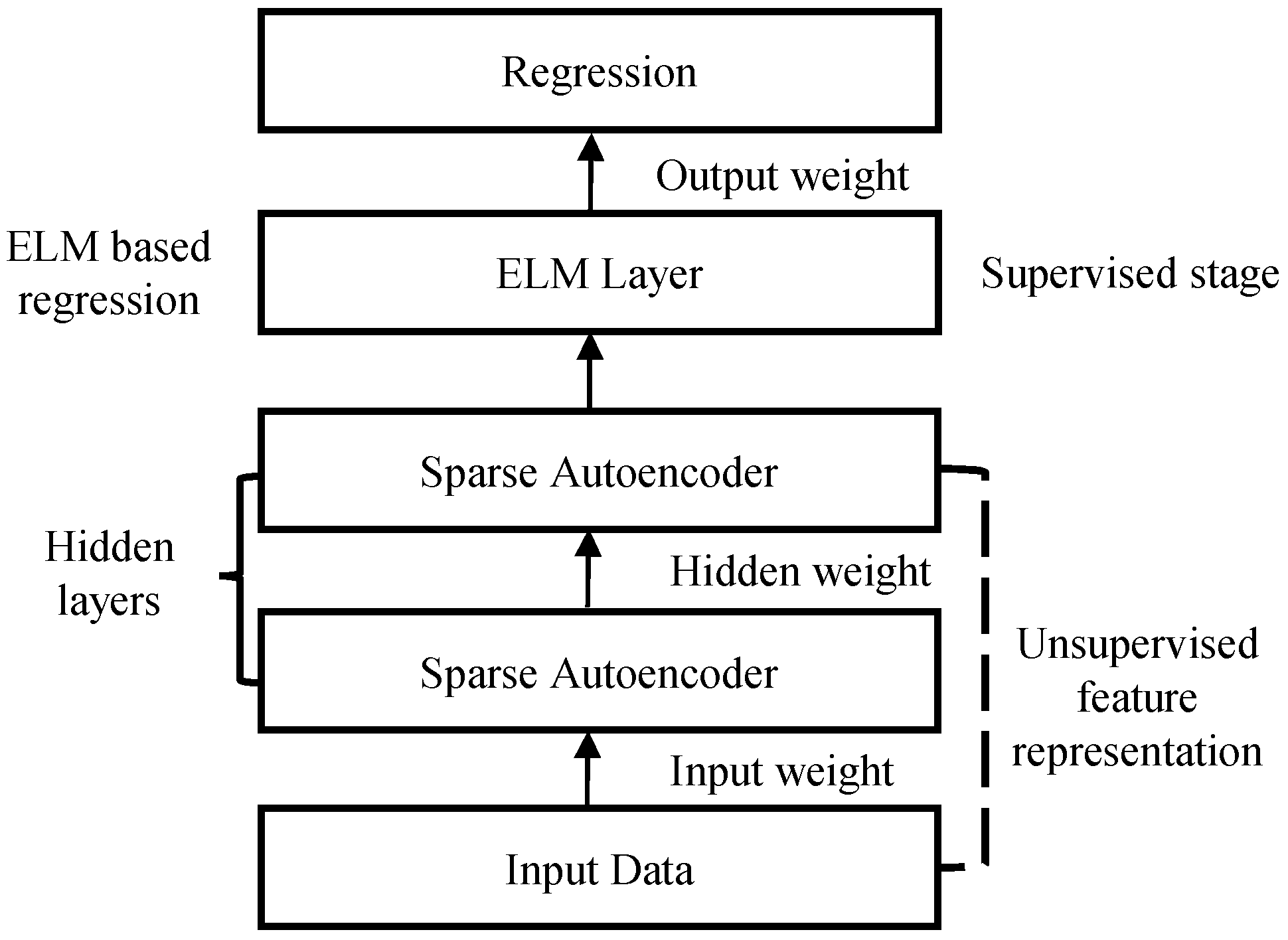
Spurred by DNNs, where the features are extracted using the multilayer framework with unsupervised initialization, Tang et al. [41] extended ELM and introduced H-ELM for multilayer perceptrons (MLPs). The entire structure of the H-ELM model is presented in Figure 1. The H-ELM framework has two steps, that is, unsupervised feature extraction, and supervised feature regression. In unsupervised feature extraction, high-level features are extracted using an ELM based autoencoder by analyzing every layer as an independent layer. The input data is introduced into the ELM feature space before feature extraction to make use of information amongst the training data. The output of the unsupervised feature extraction stage can then be used as the input to the supervised ELM regression stage [41] for the final result, based on the learning from the two stages.
5. Experimental Setup & Results
In this section, the experimental setup will be explained first. Next, we will present the performance evaluation criteria. Finally, the experimental results will be exhibited, accompanied by a short dissertation on the main findings.
5.1. Datasets
Our goal is to prove that the proposed solution can achieve comparable, if not better performance, than recently proposed deep learning methods. Hence, we needed to deploy an experimental setup that allowed a comparison with that available in the literature. To this end, we followed [27] and used UK-DALE [29] as our source dataset, so that we could perform a sound quantitative comparison between the proposed approach and that available in the literature. Each submeter in UK-DALE sampled once every 6 s. All houses recorded aggregate apparent mains power once every 6 s. Houses number 1, 2, and 5 also recorded active and reactive mains power once a second. In these houses, we downsampled 1 s active mains power to 6 s to align with the submetered data, and used this as the real aggregate data from these houses. We also aligned with the submetered data and used this as the real aggregate data from these houses by down sampling the 1 s active mains power to 6 s. We used this approach to make our results comparable with the state-of-the-art techniques. Any gaps in appliance data shorter than 3 min were assumed to be due to RF issues, and so were filled by forward-filling. Any gaps longer than 3 min were assumed to be due to the appliance and meter being switched off, and so were filled with zeros.
We used the five target appliances selected in [27] in all our experiments; namely the fridge, washing machine, dish washer, kettle, and microwave. These appliances were chosen because each is present in at least three houses in UK-DALE. This meant that for each appliance, we could train our nets on at least two houses and test on a different house. These five appliances consume a significant amount of energy, and represent a range of different power ‘signatures’ from the simple on/off of the kettle to the intricate pattern shown by the washing machine. In [27], the authors define an “appliance activation” to be the power drawn by a single appliance over one complete cycle of that appliance. We adopt the same terminology here.
In [27], the authors pointed out that artificial data had to be generated in order to regularize the training of the parameters (biases and weights) of their deep neural networks, having between 1 million and 150 million of trainable parameters. Consequently, large training datasets play a crucial role. Our approach was back-propagation free; therefore, there were fewer parameters to learn, which allowed us to use only real data during the ELM learning phase. This is a key feature of the proposed approach. For each house, we reserved the last week of data for testing and used the rest of the data for training, as in [27]. The specific houses used for training and testing are shown in Table 2.
5.2. Performance Evaluation Criteria
As described in [60], it is assumed that the most prevalent performance evaluation criteria used by non-intrusive load monitoring researchers are split into two categories. In the first one, they compare the observed aggregate power signal with the reconstructed signal after the decomposition. These metrics include:
where is the actual power of the appliance, is the estimated power after disaggregation, and is the number of examples.
The second category, on the contrary, defines how the disaggregated signal signs are assigned to each appliance, taking into account precision (P), recall (R), F-measure (F1), total energy correctly assigned (TECA), and Accuracy (A). These metrics are defined as follows:
where is the true positive that the appliance was working, is the false positive that the appliance was working, is the true negative, and is the false negative. is the number of positive cases in ground truth, and is the number of negative cases in ground truth. Moreover, is the actual power for the -th appliance at time , is the estimated power for -th appliance at time , and is the number of samples. The time period used for testing the efficiency of appliance recognition is one week. The number of appliances that can be simultaneously active, of course varies as time passes. Therefore, it is not constant during the period of time considered in the testing phase.
5.3. ELM Architectural Details
We implemented our neural nets in Python. We trained our ELMs on an NVIDIA GeForce GT 750 M GPU with 2 GB of GDDR5. On this GPU, our nets typically took 1 and 3 h to train per appliance for the shallow and hierarchical ELM architecture, respectively. We trained one ELM per given appliance. The output of the ELM was a window of the power demand of the target appliance. The input to every ELM was a window of aggregate power demand. The input window width was decided on an appliance-by-appliance basis. In particular, the duration depends on the power demand of the appliance, but the window width has to be selected to ensure that the majority of the appliance activations are captured. However, a drop in performance can be observed if the width is too large, as reported in [27], where for instance, the autoencoder for the fridge failed to learn anything useful with a window size of 1024 samples. The shallow ELM had the following structure: Input dimension determined by the appliance duration, fully connected layer with 4096 hidden nodes having Sigmoid activation function, and output dimension determined by the appliance duration. The H-ELM had the following structure: Input dimension determined by the appliance, four hidden non-linear layers with 2048 nodes having Sigmoid activation function, and output dimension determined by the appliance duration. Our approach was supervised, and the input windows were 128 input samples for the kettle, 256 samples for the microwave, 512 samples for the fridge, 768 samples for the washing machine, and 1536 samples for the dishwasher. No assumption was made on the number of appliances that can operate simultaneously. In this way, the proposed solution could work with all appliances (5 in the UK-DALE corpus) simultaneously.
5.4. Experimental Results and Discussion
For the sake of comparison, we reported results with combinatorial optimization (CO), the Factorial Hidden Markov Model (FHMM), long short-term memory (LSTM) recurrent neural networks, and autoencoder algorithms. The performance of these solutions is given as reported in [27]. It should be pointed out that there is a single LSTM per appliance in [27], and LSTMs have a number of trainable parameters that is around 1 million. There is also an autoencoder neural architecture per appliance, with a number of trainable parameters that range from 1 million to 150 million depending on the input size. The interested reader is referred to [27] for more details on both the LSTM and autoencoder training phase. The autoencoder acts as a denoiser, and it is therefore similar to our ELM-based solutions.
The disaggregation results for seen houses are shown in Table 3. The results for unseen houses during training are shown in Table 4. From the seen houses in Table 3, we observe that LSTM outperforms more conventional CO and FHMM on two-state appliances (kettle, fridge, and microwave), and it falls behind CO and FHMM on multi-state appliances (dishwasher and washing machine). The shallow ELM solution attains comparable performance with CO and FHMM, yet it is worse than the LSTM and autoencoder solutions. The proposed H-ELM instead outperforms CO, FHMM, LSTM, and the autoencoder for every appliance on F1 score, P score, accuracy, the proportion of total energy correctly assigned, and MAE, on both two-state and multi-state appliances.
It is also significant to verify the generalization capabilities on unseen houses during training. From the results reported in Table 4, we see that autoencoder outperforms CO and FHMM for every appliance on every metric, except the relative error in total energy. Instead, the H-ELM outperformed all of the other solutions, as expected. We have already demonstrated that H-ELMs are superior in performance than shallow ELMs, so we do not report ELM results for unseen houses.
Finally, we have demonstrated that ELMs can play a key role in energy disaggregation, attaining new state-of-the-art results. The importance of avoiding a cumbersome training phase can also be better appreciated by referring to a recent study about a training-less solution to non-intrusive load monitoring [61].
6. Conclusions
ELMs are a promising artificial neural network method introduced in [56] that have a high-speed learning capability, and have been employed in many tasks successfully. For instance, ELMs for wind speed forecasting were used in [62,63]. In [64], the authors apply ELMs to a state-of-charge estimation of a battery with success. ELMs were also suggested as an effective solution to guarantee the continuous flow of current supply in smart grids. In this paper, we have proposed to apply ELMs to NILM. ELMs, both in their shallow and hierarchical configurations, act as a non-linear signal enhancement system allowing us to recover the power load of the target appliance from the aggregated load. In this work, we have proposed to extend ELMs to the energy disaggregation problem, and we have reported top performance on the UK-DALE dataset. ELMs are much more straightforward to train than the deep models reported in [27], while attaining superior performance in both seen and unseen houses, and across appliances. The main advantage of ELMs over LSTMs and denoise autoencoders, is that there is no need to fine-tune the whole network by the iterative back-propagation algorithm, and this can quicken the learning speed and strengthen the generalization performance.
Finally, it is worth noting that the comparing various NILM approach can be still involved. However, many improvements have been made in recent years, and there are a lot of novel approaches, and diverse mathematical tools, that have still not been employed extensively. We believe that ELM shows great potential for NILM, and further improvement could be achieved through multi-task learning. We also believe that extreme learning machines could play a key role in the management of power consumption in industrial wireless sensor networks [65].
Author Contributions
V.M.S. conceived the main idea of the proposed work and lead the organization and writing of the paper. V.M.S. and G.R. were equally involved with setting up the experimental environment. G.R. was responsible for the experimental validation of the idea proposed in this work.
Funding
This research received no external funding.
Conflicts of Interest
The authors declare no conflict of interest.
References
- Uteley, J.; Shorrock, L. Domestic Energy Fact File 2008. Available online: http://www.bre.co.uk/page.jsp?id=879 (accessed on 8 July 2018).
- EIA Energy Consumption Report. Available online: https://www.eia.gov/totalenergy/data/annual/pdf/sec2.pdf (accessed on 8 July 2018).
- EU Energy Consumption. Available online: http://www.eea.europa.eu/data-and-maps/figures/final-energy-consumption-by-sector-eu-27 (accessed on 8 July 2018).
- EIA Residential Report. Available online: https://www.eia.gov/consumption/residential/index.php (accessed on 8 July 2018).
- Meyers, R.J.; Williams, E.D.; Matthews, H.S. Scoping the potential of monitoring and control technologies to reduce energy use in homes. Energy Build. 2010, 42, 563–569. [Google Scholar] [CrossRef]
- Darby, S. The Effectiveness of Feedback on Energy Consumption: A Review for DEFRA of the Literature on Metering. 2006. Available online: https://www.eci.ox.ac.uk/research/energy/downloads/smart-metering-report.pdf (accessed on 8 July 2018).
- Abrahamse, W.; Steg, L.; Vlek, C.; Rothengatter, T. A review of intervention studies aimed at household energy conservation. J. Environ. Psychol. 2005, 25, 273–291. [Google Scholar] [CrossRef]
- Yu, L.; Li, H.; Feng, X.; Duan, J. Nonintrusive appliance load monitoring for smart homes: recent advances and future issues. IEEE Instrum. Meas. Mag. 2016, 19, 56–62. [Google Scholar] [CrossRef]
- Soetedjo, A.; Nakhoda, Y.I.; Saleh, C. Embedded Fuzzy Logic Controller and Wireless Communication for Home Energy Management Systems. Electronics 2018, 7, 189. [Google Scholar] [CrossRef]
- Issi, F.; Kaplan, O. The Determination of Load Profiles and Power Consumptions of Home Appliances. Energies 2018, 11, 607. [Google Scholar] [CrossRef]
- Manivannan, M.; Najafi, B.; Rinaldi, F. Machine Learning-Based Short-Term Prediction of Air-Conditioning Load through Smart Meter Analytics. Energies 2017, 10, 1905. [Google Scholar] [CrossRef]
- Jain, R.K.; Smith, K.M.; Culligan, P.J.; Taylor, J.E. Forecasting energy consumption of multi-family residential buildings using support vector regression: Investigating the impact of temporal and spatial monitoring granularity on performance accuracy. Appl. Energy 2014, 123, 168–178. [Google Scholar] [CrossRef]
- Paterson, G.; Mumovic, D.; Das, P.; Kimpian, J. Energy use predictions with machine learning during architectural concept design. Sci. Technol. Built Environ. 2017, 23, 1036–1048. [Google Scholar] [CrossRef] [Green Version]
- Karatasou, S.; Santamouris, M.; Geros, V. Modeling and predicting building’s energy use with artificial neural networks: Methods and results. Energy Build. 2006, 38, 949–958. [Google Scholar] [CrossRef]
- Hart, G.W. Nonintrusive appliance load monitoring. Proc. IEEE 1992, 80, 1870–1891. [Google Scholar] [CrossRef]
- Zeifman, M.; Roth, K. Nonintrusive appliance load monitoring: Review and outlook. IEEE Trans. Consum. Electron. 2011, 57, 76–84. [Google Scholar] [CrossRef]
- Zoha, A.; Gluhak, A.; Imran, M.A.; Rajasegarar, S. Non-intrusive load monitoring approaches for disaggregated energy sensing: A survey. Sensors 2012, 12, 16838–16866. [Google Scholar] [CrossRef] [PubMed] [Green Version]
- Chang, H.-H.; Lian, K.-L.; Su, Y.-C.; Lee, W.-J. Power-spectrum-based wavelet transform for nonintrusive demand monitoring and load identification. IEEE Trans. Ind. Appl. 2014, 50, 2081–2089. [Google Scholar] [CrossRef]
- Haq, A.U.; Jacobsen, H.-A. Prospects of Appliance-Level Load Monitoring in Off-the-Shelf Energy Monitors: A Technical Review. Energies 2018, 11, 189. [Google Scholar] [CrossRef]
- Meehan, P.; McArdle, C.; Daniels, S. An Efficient, Scalable Time-Frequency Method for Tracking Energy Usage of Domestic Appliances Using a Two-Step Classification Algorithm. Energies 2014, 7, 7041–7066. [Google Scholar] [CrossRef] [Green Version]
- Kwak, Y.; Hwang, J.; Lee, T. Load Disaggregation via Pattern Recognition: A Feasibility Study of a Novel Method in Residential Building. Energies 2018, 11, 1008. [Google Scholar] [CrossRef]
- Norford, L.K.; Mabey, N. Non-Intrusive Electric Load Monitoring in Commercial Buildings. In Proceedings of the Eighth Symposium on Improving Building Systems in Hot and Humid Climates, Dallas, TX, USA, 13–14 May 1992; pp. 133–140. [Google Scholar]
- Zia, T.; Bruckner, D.; Zaidi, A.A. Hidden Markov Model Based Procedure for Identifying Household Electric Loads. In Proceedings of the 37th Annual Conference on IEEE Industrial Electronics Society, Melbourne, Australia, 7–10 November 2011; pp. 3218–3322. [Google Scholar]
- Onoda, T.; Rätsch, G.; Müller, K.R. Applying support vector machines and boosting to a non-intrusive monitoring system for household electric appliances with inverters. In Proceedings of the Second ICSC Symposium on Neural Computation, Berlin, Germany, 23–26 May 2000. [Google Scholar]
- Fomby, T.B.; Barber, T. K-Nearest Neighbors Algorithm: Prediction and Classification; Southern Methodist University: Dallas, TX, USA, 2008; pp. 1–5. [Google Scholar]
- Gomes, L.; Fernandes, F.; Sousa, T.; Silva, M.; Morais, H.; Vale, Z.; Ramos, C. Contextual intelligent load management with ANN adaptive learning module. In Proceedings of the 16th International Conference on Intelligent System Application to Power Systems (ISAP 2011), Hersonissos, Greece, 25–28 September 2011. [Google Scholar] [CrossRef]
- Kelly, J.; Knottenbelt, W. Neural NILM: Deep neural networks applied to energy disaggregation. In Proceedings of the 2nd ACM International Conference on Embedded Systems for Energy-Efficient Built Environments, Seoul, Korea, 4–5 November 2015; ACM: New York, NY, USA, 2015; pp. 55–64. [Google Scholar]
- Ruzzelli, A.G.; Nicolas, C.; Schoofs, A.; O’Hare, G.M. Real-time recognition and profiling of appliances through a single electricity sensor. In Proceedings of the 7th Annual IEEE Communications Society Conference on Sensor, Mesh and Ad Hoc Communications and Networks, Boston, MA, USA, 21–25 June 2010. [Google Scholar] [CrossRef]
- Nalmpantis, C.; Vrakas, D. Machine learning approaches for non-intrusive load monitoring: from qualitative to quantitative comparison. Artif. Intell. Rev. 2018. [Google Scholar] [CrossRef]
- Zeifman, M. Disaggregation of home energy display data using probabilistic approach. IEEE Trans. Consum. Electron. 2012, 58, 23–31. [Google Scholar] [CrossRef]
- Bengio, Y. Learning deep architectures for AI. Found Trends Mach. Found. Trends Mach. Learn. 2009, 2, 1–127. [Google Scholar] [CrossRef]
- Hinton, G.E.; Deng, L.; Yu, D.; Dahl, G.; Mohamed, A.-R.; Jaitly, N.; Senior, A.; Vanhoucke, V.; Nguyen, P.; Sainath, T.; et al. Deep neural networks for acoustic modeling in speech recognition: The shared views of four research groups. IEEE Signal Process Mag. 2012, 29, 82–97. [Google Scholar] [CrossRef]
- Siniscalchi, S.M.; Salerno, V.M. Adaptation to new microphones using artificial neural networks with trainable activation functions. IEEE Trans. Neural Netw. Learn. Syst. 2017, 28, 1959–1965. [Google Scholar] [CrossRef] [PubMed]
- LeCun, Y.; Bottou, L.; Bengio, Y.; Haffner, P. Gradient-based learning applied to document recognition. Proc. IEEE 1998, 86, 2278–2324. [Google Scholar] [CrossRef] [Green Version]
- Krizhevsky, A.; Sutskever, I.; Hinton, G.E. Imagenet classification with deep convolutional neural networks. In Proceedings of the 25th International Conference on Neural Information Processing Systems, Lake Tahoe, NV, USA, 3–6 December 2012; pp. 1097–1105. [Google Scholar]
- Hochreiter, S.; Schmidhuber, J. Long short-term memory. Neural Comput. 1997, 9, 1735–1780. [Google Scholar] [CrossRef] [PubMed]
- Mauch, L.; Yang, B. A new approach for supervised power disaggregation by using a deep recurrent LSTM network. In Proceedings of the 3rd IEEE Global Conference on Signal and Information Processing, Orlando, FL, USA, 14–16 December 2015; pp. 63–67. [Google Scholar]
- Zhang, C.; Zhong, M.; Wang, Z.; Goddard, N.; Sutton, C. Sequence-to-point learning with neural networks for nonintrusive load monitoring. In Proceedings of the AAAI-18: Thirty-Second AAAI Conference on Artificial Intelligence, New Orleans, LA, USA, 2–7 February 2018. [Google Scholar]
- Huang, G.-B. An insight into extreme learning machines: random neurons, random features and kernels. Cognit. Comput. 2014, 6, 376–390. [Google Scholar] [CrossRef]
- Huang, Z.; Yu, Y.; Gu, J.J.; Liu, H. An efficient method for traffic sign recognition based on extreme learning machine. IEEE Trans. Cybern. 2017, 47, 920–933. [Google Scholar] [CrossRef] [PubMed]
- Tang, J.; Deng, C.; Huang, G.-B. Extreme learning machine for multilayer perceptron. IEEE Trans. Neural Netw. Learn. Syst. 2016, 27, 809–821. [Google Scholar] [CrossRef] [PubMed]
- Sun, F.; Liu, C.; Huang, W.; Zhang, J. Object classification and grasp planning using visual and tactile sensing. IEEE Trans. Syst. Man Cybern. Syst. 2016, 46, 969–979. [Google Scholar] [CrossRef]
- Kasun, L.L.C.; Zhou, H.; Huang, G.-B.; Vong, C.M. Representational learning with ELMs for big data. IEEE Intell. Syst. 2013, 28, 31–34. [Google Scholar]
- Zhao, W.; Beach, T.H.; Rezgui, Y. Optimization of potable water distribution and wastewater collection networks: A systematic review and future research directions. IEEE Trans. Syst. Man Cybern. Syst. 2016, 46, 659–681. [Google Scholar] [CrossRef]
- Wang, D.; Bischof, L.; Lagerstrom, R.; Hilsenstein, V.; Hornabrook, A.; Hornabrook, G. Automated Opal Grading by Imaging and Statistical Learning. IEEE Trans. Syst. Man Cybern. Syst. 2016, 46, 185–201. [Google Scholar] [CrossRef]
- Liu, D.; Wei, Q.; Yan, P. Generalized policy iteration adaptive dynamic programming for discrete time nonlinear systems. IEEE Trans. Syst. Man Cybern. Syst. 2015, 45, 1577–1591. [Google Scholar] [CrossRef]
- Huang, G.-B.; Zhou, H.; Ding, X.; Zhang, R. Extreme learning machine for regression and multiclass classification. IEEE Trans. Syst. Man Cybern. Part B Cybern. 2012, 42, 513–529. [Google Scholar] [CrossRef] [PubMed]
- Kelly, J.; Knottenbelt, W. The UK-DALE dataset, domestic appliance-level electricity demand and whole-house demand from five UK homes. Sci. Data 2015, 2, 150007. [Google Scholar] [CrossRef] [PubMed]
- Kim, H.; Marwah, M.; Arlitt, M.; Lyon, G.; Han, J. Unsupervised disaggregation of low frequency power measurements. In Proceedings of the 2011 SIAM International Conference on Data Mining, Mesa, AZ, USA, 28–30 April 2011; pp. 747–758. [Google Scholar]
- Kolter, J.Z.; Johnson, M.J. Redd: A public data set for energy disaggregation research. In Proceedings of the Workshop on Data Mining Applications in Sustainability, San Diego, CA, USA, 21 August 2011. [Google Scholar]
- Kolter, J.Z.; Jaakkola, T. Approximate inference in additive factorial HMMs with application to energy disaggregation. In Proceedings of the 15th International Conference on Artificial Intelligence and Statistics (AISTATS), La Palma, Canary Islands, Spain, 21–23 April 2012; pp. 1472–1482. [Google Scholar]
- Parson, O.; Ghosh, S.; Weal, M.; Rogers, A. Using hidden Markov models for iterative non-intrusive appliance monitoring. In Proceedings of the Neural Information Processing Systems workshop on Machine Learning for Sustainability, Sierra Nevada, Spain, 16–17 December 2011. [Google Scholar]
- Parson, O.; Ghosh, S.; Weal, M. Rogers, Non-intrusive load monitoring using prior models of general appliance types. In Proceedings of the Twenty-Sixth AAAI Conference on Artificial Intelligence, Toronto, ON, Canada, 22–26 July 2012; AAAI Press: Palo Alto, CA, USA, 2012; pp. 356–362. [Google Scholar]
- Egarter, D.; Bhuvana, V.P.; Elmenreich, W. PALDi: online load disaggregation via particle filtering. IEEE Trans. Instrum. Meas. 2015, 64, 467–477. [Google Scholar] [CrossRef]
- Paradiso, F.; Paganelli, F.; Giuli, D.; Capobianco, S. Context-based energy disaggregation in smart homes. Future Internet 2016, 8, 4. [Google Scholar] [CrossRef]
- Aiad, M.; Lee, P.H. Unsupervised approach for load disaggregation with devices interactions. Energy Build. 2016, 116, 96–103. [Google Scholar] [CrossRef]
- Makonin, S.; Popowich, F.; Bajic, I.V.; Gill, B. ; Bartram, L. Exploiting HMM sparsity to perform online real- time nonintrusive load monitoring. IEEE Trans. Smart Grid 2016, 7, 2575–2585. [Google Scholar] [CrossRef]
- Lange, H.; Bergés, M. The neural energy decoder: energy disaggregation by combining binary subcomponents. In Proceedings of the NILM2016 3rd International Workshop on Non-Intrusive Load Monitoring, Vancouver Canada, 14–15 May 2016. [Google Scholar]
- Beck, A.; Teboulle, M. A fast iterative shrinkage-thresholding algorithm for linear inverse problems. SIAM J. Imaging Sci. 2009, 2, 183–202. [Google Scholar] [CrossRef]
- Bonfigli, R.; Squartini, S.; Fagiani, M.; Piazza, F. Unsupervised algorithms for non-intrusive load monitoring: An up-to-date overview. In Proceedings of the 2015 IEEE 15th International Conference on Environment and Electrical Engineering (EEEIC), Rome, Italy, 10–13 June 2015. [Google Scholar] [CrossRef]
- Zhao, B.; Stankovic, L.; Stankovic, V. On a Training-Less Solution for Non-Intrusive Appliance Load Monitoring Using Graph Signal Processing. IEEE Access 2016, 4, 1784–1799. [Google Scholar] [CrossRef]
- Zhou, J.; Sun, N.; Jia, B.; Peng, T. A Novel Decomposition-Optimization Model for Short-Term Wind Speed Forecasting. Energies 2018, 11, 1752. [Google Scholar] [CrossRef]
- Wang, R.; Li, J.; Wang, J.; Gao, C. Research and Application of a Hybrid Wind Energy Forecasting System Based on Data Processing and an Optimized Extreme Learning Machine. Energies 2018, 11, 1712. [Google Scholar] [CrossRef]
- Chin, C.S.; Gao, Z. State-of-Charge Estimation of Battery Pack under Varying Ambient Temperature Using an Adaptive Sequential Extreme Learning Machine. Energies 2018, 11, 711. [Google Scholar] [CrossRef]
- Collotta, M.; Pau, G.; Salerno, V.M.; Scatà, G. A fuzzy based algorithm to Manage Power Consumption in Industrial Wireless Sensor Networks. In Proceedings of the 2011 9th IEEE International Conference on Industrial Informatics, Lisbon, Portugal, 26–29 July 2011. [Google Scholar] [CrossRef]
Figure 1.
Hierarchical extreme learning machine (H-ELM) architecture.


Table 1.
A simulated example of the energy disaggregation problem.
| Timestamp (20 min) | Total Consumption | Oven | TV | Dishwasher | Laptop | Others |
|---|---|---|---|---|---|---|
| t0 | 540 | 0 | 130 | 390 | 20 | 0 |
| t1 | 540 | 0 | 130 | 390 | 20 | 0 |
| t2 | 600 | 80 | 0 | 390 | 50 | 80 |
| t3 | 500 | 80 | 120 | 300 | 50 | 50 |
| t4 | 800 | 450 | 0 | 300 | 50 | 0 |
| t5 | 800 | 450 | 0 | 300 | 50 | 0 |
| t6 | 750 | 450 | 0 | 300 | 0 | 0 |
| t7 | 830 | 450 | 80 | 300 | 0 | 0 |
| t8 | 750 | 450 | 0 | 300 | 0 | 0 |
| … | … | … | … | … | … | … |
Table 2.
Houses used for training and testing.
| Appliance | Training | Testing |
|---|---|---|
| Kettle | 1, 2, 3, 4 | 5 |
| Fridge | 1, 2, 4 | 5 |
| Washing Machine | 1, 5 | 2 |
| Microwave | 1, 2 | 5 |
| Dish washer | 1, 2 | 5 |
Table 3.
Disaggregation performance for seen houses during training.
| Technique | Appliance | F1 | P | R | A | RET | TECA | MAE |
|---|---|---|---|---|---|---|---|---|
| CO | Kettle | 0.31 | 0.45 | 0.25 | 0.99 | 0.43 | 0.93 | 65 |
| Dish Washer | 0.11 | 0.07 | 0.50 | 0.69 | 0.28 | 0.90 | 75 | |
| Fridge | 0.52 | 0.50 | 0.54 | 0.61 | 0.26 | 0.94 | 50 | |
| Microwave | 0.33 | 0.24 | 0.70 | 0.98 | 0.85 | 0.92 | 68 | |
| Washing Machine | 0.13 | 0.08 | 0.56 | 0.69 | 0.65 | 0.92 | 88 | |
| FHMM | Kettle | 0.28 | 0.30 | 0.28 | 0.99 | 0.57 | 0.91 | 82 |
| Dish Washer | 0.08 | 0.04 | 0.78 | 0.37 | 0.66 | 0.85 | 111 | |
| Fridge | 0.47 | 0.39 | 0.63 | 0.46 | 0.50 | 0.91 | 69 | |
| Microwave | 0.43 | 0.35 | 0.69 | 0.99 | 0.80 | 0.93 | 54 | |
| Washing Machine | 0.11 | 0.06 | 0.87 | 0.39 | 0.76 | 0.88 | 138 | |
| Autoencoder | Kettle | 0.48 | 1.00 | 0.39 | 0.99 | 0.02 | 0.98 | 16 |
| Dish Washer | 0.66 | 0.45 | 0.99 | 0.95 | –0.34 | 0.97 | 21 | |
| Fridge | 0.81 | 0.83 | 0.79 | 0.85 | –0.35 | 0.97 | 25 | |
| Microwave | 0.62 | 0.50 | 0.86 | 0.99 | –0.06 | 0.99 | 13 | |
| Washing Machine | 0.25 | 0.15 | 0.99 | 0.76 | 0.18 | 0.96 | 44 | |
| LSTM | Kettle | 0.71 | 0.91 | 0.63 | 1.00 | 0.36 | 0.98 | 23 |
| Dish Washer | 0.06 | 0.03 | 0.63 | 0.35 | 0.76 | 0.83 | 130 | |
| Fridge | 0.69 | 0.71 | 0.67 | 0.76 | –0.22 | 0.96 | 34 | |
| Microwave | 0.42 | 0.28 | 0.92 | 0.98 | 0.50 | 0.97 | 22 | |
| Washing Machine | 0.09 | 0.05 | 0.62 | 0.31 | 0.73 | 0.88 | 133 | |
| Shallow ELM | Kettle | 0.27 | 0.23 | 0.24 | 0.99 | 0.58 | 0.91 | 81 |
| Dish Washer | 0.09 | 0.06 | 0.81 | 0.33 | 0.62 | 0.85 | 112 | |
| Fridge | 0.42 | 0.23 | 0.67 | 0.47 | 0.48 | 0.92 | 68 | |
| Microwave | 0.41 | 0.45 | 0.71 | 0.98 | 0.81 | 0.90 | 52 | |
| Washing Machine | 0.15 | 0.12 | 0.82 | 0.42 | 0.72 | 0.82 | 137 | |
| H-ELM | Kettle | 0.72 | 1.00 | 0.70 | 1.00 | 0.01 | 0.98 | 15 |
| Dish Washer | 0.75 | 0.89 | 0.99 | 0.98 | –0.54 | 0.98 | 19 | |
| Fridge | 0.89 | 0.88 | 0.80 | 0.88 | –0.38 | 0.98 | 20 | |
| Microwave | 0.66 | 0.52 | 0.87 | 0.99 | –0.05 | 0.99 | 12 | |
| Washing Machine | 0.50 | 0.73 | 0.99 | 0.76 | 0.09 | 0.97 | 27 |
Table 4.
Disaggregation performance for unseen houses during training. This evaluation is essential to assess the generalization capability of the pattern recognition technique.
Table 4.
Disaggregation performance for unseen houses during training. This evaluation is essential to assess the generalization capability of the pattern recognition technique.
| Technique | Appliance | F1 | P | R | A | RET | TECA | MAE |
|---|---|---|---|---|---|---|---|---|
| CO | Kettle | 0.31 | 0.23 | 0.46 | 0.99 | 0.85 | 0.94 | 73 |
| Dish Washer | 0.11 | 0.06 | 0.67 | 0.64 | 0.62 | 0.94 | 74 | |
| Fridge | 0.35 | 0.30 | 0.41 | 0.45 | 0.37 | 0.94 | 73 | |
| Microwave | 0.05 | 0.03 | 0.35 | 0.98 | 0.97 | 0.93 | 89 | |
| Washing Machine | 0.10 | 0.06 | 0.48 | 0.88 | 0.73 | 0.93 | 39 | |
| FHMM | Kettle | 0.19 | 0.14 | 0.29 | 0.99 | 0.88 | 0.92 | 98 |
| Dish Washer | 0.05 | 0.03 | 0.49 | 0.33 | 0.75 | 0.91 | 110 | |
| Fridge | 0.55 | 0.40 | 0.86 | 0.50 | 0.57 | 0.94 | 67 | |
| Microwave | 0.01 | 0.01 | 0.34 | 0.91 | 0.99 | 0.84 | 195 | |
| Washing Machine | 0.08 | 0.04 | 0.64 | 0.79 | 0.86 | 0.88 | 67 | |
| Autoencoder | Kettle | 0.93 | 1.00 | 0.87 | 1.00 | 0.13 | 1.00 | 6 |
| Dish Washer | 0.44 | 0.29 | 0.99 | 0.92 | –0.33 | 0.98 | 24 | |
| Fridge | 0.87 | 0.85 | 0.88 | 0.90 | –0.38 | 0.98 | 26 | |
| Microwave | 0.26 | 0.15 | 0.94 | 0.99 | 0.73 | 0.99 | 9 | |
| Washing Machine | 0.13 | 0.07 | 1.00 | 0.82 | 0.48 | 0.96 | 24 | |
| LSTM | Kettle | 0.93 | 0.96 | 0.91 | 1.00 | 0.57 | 0.99 | 16 |
| Dish Washer | 0.08 | 0.04 | 0.87 | 0.30 | 0.87 | 0.86 | 168 | |
| Fridge | 0.74 | 0.71 | 0.77 | 0.81 | –0.25 | 0.97 | 36 | |
| Microwave | 0.13 | 0.07 | 0.99 | 0.98 | 0.88 | 0.98 | 20 | |
| Washing Machine | 0.03 | 0.01 | 0.73 | 0.23 | 0.91 | 0.81 | 109 | |
| H-ELM | Kettle | 0.95 | 1.00 | 0.92 | 1.00 | 0.10 | 1.00 | 4 |
| Dish Washer | 0.55 | 0.35 | 1.00 | 1.00 | –0.28 | 0.98 | 22 | |
| Fridge | 0.89 | 0.90 | 0.92 | 0.94 | –0.22 | 0.98 | 23 | |
| Microwave | 0.36 | 0.32 | 0.98 | 0.99 | 0.65 | 0.99 | 7 | |
| Washing Machine | 0.43 | 0.10 | 1.00 | 0.84 | 0.51 | 0.97 | 21 |
© 2018 by the authors. Licensee MDPI, Basel, Switzerland. This article is an open access article distributed under the terms and conditions of the Creative Commons Attribution (CC BY) license (http://creativecommons.org/licenses/by/4.0/).
Share and Cite
MDPI and ACS Style
Salerno, V.M.; Rabbeni, G. An Extreme Learning Machine Approach to Effective Energy Disaggregation. Electronics 2018, 7, 235. https://0-doi-org.brum.beds.ac.uk/10.3390/electronics7100235
AMA Style
Salerno VM, Rabbeni G. An Extreme Learning Machine Approach to Effective Energy Disaggregation. Electronics. 2018; 7(10):235. https://0-doi-org.brum.beds.ac.uk/10.3390/electronics7100235
Chicago/Turabian StyleSalerno, Valerio Mario, and Graziella Rabbeni. 2018. "An Extreme Learning Machine Approach to Effective Energy Disaggregation" Electronics 7, no. 10: 235. https://0-doi-org.brum.beds.ac.uk/10.3390/electronics7100235
Note that from the first issue of 2016, this journal uses article numbers instead of page numbers. See further details here.