Day Ahead Real Time Pricing and Critical Peak Pricing Based Power Scheduling for Smart Homes with Different Duty Cycles

Abstract

In this paper, we propose a demand side management (DSM) scheme in the residential area for electricity cost and peak to average ratio (PAR) alleviation with maximum users’ satisfaction. For this purpose, we implement state-of-the-art algorithms: enhanced differential evolution (EDE) and teacher learning-based optimization (TLBO). Furthermore, we propose a hybrid technique (HT) having the best features of both aforementioned algorithms. We consider a system model for single smart home as well as for a community (multiple homes) and each home consists of multiple appliances with different priorities. The priority is assigned (to each appliance) by electricity consumers and then the proposed scheme finds an optimal solution according to the assigned priorities. Day-ahead real time pricing (DA-RTP) and critical peak pricing (CPP) are used for electricity cost calculation. To validate our proposed scheme, simulations are carried out and results show that our proposed scheme efficiently achieves the aforementioned objectives. However, when we perform a comparison with existing schemes, HT outperforms other state-of-the-art schemes (TLBO and EDE) in terms of electricity cost and PAR reduction while minimizing the average waiting time.

1. Introduction

The dream of smart electric power system is become true in the past few decades with the emergence of smart grid (SG). SG provides the vision of integrating sensing and communication technologies for controlled power flow between the utility and a consumer [1]. Moreover, it revolutionized the traditional grid by enabling bi-directional communication in the electricity system. Additionally, the use of sensing and communication technologies and control mechanisms enabled real time monitoring and distribution of electricity at consumer level in more friendly way [2]. Furthermore, it has the ability of self healing, attack resistance and capable to store and generate all types of electricity in real time.

With the emergence of SG, it is very convenient for the utility to provide consumers electricity based on the time dependent prices which includes real time and day ahead pricing. By receiving information from the utility, consumer can adjust the operations of an appliance according to the pricing scheme [3]. Moreover, the advanced metering infrastructure (AMI) allows the consumers to store the information and make timely decisions. The stored data helps to optimally schedule the appliances for minimum electricity cost using the energy management controller (EMC). This is a programmable logic controller which allows the consumer to implement the demand response algorithms for controlling the operations of smart devices as per the requirements.

In the era of SG, demand side management (DSM) plays an important role to achieve a balanced load on the utility. Due to DSM strategies, it is possible for end consumers to minimize the electricity cost and PAR. However, customer participation is an important aspect to successfully implement the DSM strategies. Moreover, it is necessary to examine the behavior of consumers for predicting the habitual energy consumption pattern [1].

Furthermore, demand response (DR) programs are offered helping end users to reduce peak power demand in peak time slots. The DR consists of incentive and price-based programs. In the former, utility provides the monetary incentives to a consumer for minimizing the load over specific time intervals [2,3]. However, to achieve this objective, an agreement between the consumer and utility is necessary [4]. In the latter, electricity consumers are offered with time-varying prices according to the power consumption pattern. As, electricity price varies dynamically over the time period of day, week or month and every consumer wants to operate appliances at the lowest pricing hour. Thus price-based scheme motivates the consumer to schedule appliances from on-peak to off-peak hours [5].

Different pricing schemes are interchangeably used by the electricity market including critical peak pricing (CPP), time of use (ToU), real time pricing (RTP) and inclined block rate (IBR). In the implementation of CPP, it is very difficult to select a suitable critical day because CPP is a dynamic pricing signal which is based on ToU and RTP. Moreover, it augments a time invariant structure with high price during the period of system stress [6]. Moreover, the CPP is not economical as compared to RTP; however, it reduces the price risk associated with RTP by reflecting the short-term cost of critical periods. The price of CPP moments is double as compared to day ahead RTP (DA-RTP). In the proposed model, both pricing signals: CPP and DA-RTP are implemented for calculating the electricity cost.

Research community is striving hard to optimize the scheduling of appliances for efficient and cost effective electricity consumption. In this regard, various optimization strategies are proposed for instance in [7,8], an optimization-based model is used to shift the load from on-peak to off-peak hours. Authors used the concept of agents to manage the electricity load and generation. Moreover, the electric vehicles are used as mobile storage to provide electricity in ON-peak hours to achieve a flattened electric load curve. Similarly, Mitra et al. used the load shifting technique to decrease the PAR and electricity cost [9]. The authors used a modified form of the particle swarm optimization (PSO) for DSM to reduce the utility production cost and minimize the peak demand.

However, in the existing state of the art schemes [7,8,9], when consumer minimizes the electricity cost, the average waiting time increases resulting high discomfort. Moreover, the sudden shift of load from off-peak to on-peak hours results in the generation of peaks. To bring the balance between electricity consumption, peak demand and user satisfaction, a dire need of an efficient algorithm emerges which can satisfy the demands of the consumers.

To overcome the aforesaid issues, we have implemented two heuristic algorithms including TLBO and EDE, to solve the electricity cost and PAR minimization problem. We propose a hybrid technique (HT) by combining the best properties of TLBO and EDE. These algorithms are preferred over PSO and other heuristic techniques due to their self-organization, self-optimization, self-protection and self-healing abilities [10]. These algorithms are tested via simulations for a home energy management controller (HEMC) under DA-RTP and CPP. The results demonstrate that significant reduction in electricity cost and PAR is observed along with the considerable improvement in the user satisfaction. The key contributions of this work are:

• The reduction of electricity cost and minimization of PAR based on the consumer defined priorities for each appliance.
• A hybrid meta-heuristic technique is developed to optimize the schedule of shift-able appliances for achieving less electricity cost along with minimum waiting time for maximum user comfort.
• HT, TLBO and EDE are implemented for multiple homes to analyze the performance of each algorithm against for different number of appliances.
• Extensive simulations in MATLAB are performed to check the performance of HT, TLBO and EDE against electricity consumption cost, PAR, and waiting time.

The rest of the work is organized as follows: Section 2 describes the related work, the problem description is in Section 3 and Section 4 deals with problem formulation, system model in Section 5, Section 6 describes proposed solution. Simulation results and discussion in Section 7, Section 8 presents the feasible region and finally, Section 9 concludes the work.

2. Related Work

In the literature, many DSM-based load scheduling techniques are presented to reduce the electricity bill and PAR. A Home energy management system (HEMS) plays a crucial role in residential scheduling. In this regard, some of the related work is presented below.

Ahmed et al. in [11] focused on the DSM for plug-in hybrid electric vehicle (PHEV) charging at low voltage transformer. The primary objectives are to flatten the electricity load curve and fulfill the consumers’ requirement for PHEV charging in OFF-peak hours. A convex programming is used to solve this load management problem. Simulation results show that the proposed algorithm efficiently achieves the desired power load curve.

A distributed algorithm used to manage sparse load shifting for DSM [12]. Authors make the contribution in three forms: (i) remodel the DSM to improve sparsity, (ii) a bidirectional framework to seek the Nash equilibrium and (iii) Newton method used to accelerate the convergence of coordination updates on the supply side. The objective of this work includes the scheduling of home appliances for the purpose of cost reduction. This way the consumer helps to achieve maximum user comfort by implementing the sparse load shifting techniques.

Authors in [13] use stackelberg game theory approach for appliance scheduling; using this concept of game theory, a relationship is created between the energy supplier and the consumer. Authors solved the problem of multiple appliances by considering the demand side along with market and supply side. The authors also covered a new dimension for improving the utility companies’ profit. The authors propose a decision process for both demand and supply side as a multi-leader multi-follower stakelberg game.

In [14], the authors used a genetic algorithm (GA) in DSM and benefited with an overall reduction of 21.91%. The load is divided into three service areas: industrial, residential and commercial. The use of electricity in peak hours vary in every service area with the objective to minimize the power utilization during the peak hours.

Authors in [15] proposed a scheduling model for appliances. Dynamic prices are considered for shifting the load from on-peak to off-peak hours. In this scheme, an optimization model is proposed which minimizes the electricity cost for the consumer. Moreover, different pricing schemes are applied in this model to make it more realistic. Additionally, user comfort and social welfare are also incorporated in this model. However, PAR is not considered in this model.

Electricity consumption cost is minimized by appliance scheduling in [16]. They considered twenty-four appliances for scheduling with the aim of reducing energy consumption. Simulation result shows that BPSO performs well as compared to GA and WDO. However, user comfort is not considered in this work.

The authors in [17] proposed a model that calculates robust price for consumers using day ahead pricing (DAP). Moreover, convergent distribution algorithm is used to find a robust price for the consumer. This algorithm significantly reduced the electricity consumption cost and provided a reliable estimated production cost to the energy supplier. The DSM mainly focuses on calculating an optimal policy for monetary saving on the consumer side. The distributed robust algorithm has very little computational complexity and a significant monetary saving.

An electricity consumer can reduce its energy consumption cost by scheduling the appliances according to electricity tariff and controlling the charging and discharging of energy storage devices. Proximal decomposition algorithm (PDA) allowed a consumer to update its energy consumption pattern. Simulation results show that PDA minimizes the energy consumption cost and peak load of the system [18].

The authors of [19] proposed an optimization model to utilize the energy optimally in smart homes. This optimization model is based on multi-objective mixed integer nonlinear programming (MO-MINLP) technique. The proposed model minimizes the tradeoff between energy consumption cost and user comfort. The MO-MINLP based smart energy management system (EMS) tests different residential loads and checks its performance through different operating conditions. Simulations are conducted to verify the efficiency and robustness of the proposed model.

In [20], the authors reduced the peak demand by shifting the appliances. They considered the default scenario with finite delay requests and compressed demand scenarios. Recursive formulas are used to calculate the peak demand which show an efficient reduction in the peak demand for a finite number of devices. However, in the proposed scheme system complexity and computational time are increased. Authors presented an energy management model, which is based on co-evolutionary PSO. This optimization technique is used to schedule the “must-run” resistive load and the load associated with PHEV. The consumer defines monetary benefits of the energy usage [21]. Yang et al. proposed an improved form of PSO to schedule the appliances [22]. This work considers the CPP, ToU and demand response signals to minimize the cost and PAR. Authors also analyze the effect of energy management on distribution transformer. The proposed algorithm is also favorable for reducing the PAR and cost. An enhanced GA-based EMS is proposed in [23] to control home appliance power consumption. In this work, RTP signals are used to calculate the electricity cost.

It is observed from the literature, research community is working to find an optimal solution for energy management problems. In this regard, heuristics optimization algorithms are used in recent studies [8,9,14,16,17] due to their abilities of self-healing, self-adaptation and low computational complexity. Moreover, mathematical techniques are also implemented for energy management [11,19]; however, when size of the problem increases, high computational complexity is the limitation of mathematical techniques.

3. Problem Description

In SG, energy optimization is a challenging task due to randomness in consumers’ energy consumption pattern. Mathematical optimization techniques are not considered feasible due to their high computational complexity. To tackle aforementioned issues, heuristic techniques are widely adopted due to their self-adaptive behavior during exploration and exploitation of the search space. The DSM deals with the activities that modify the electricity consumption pattern to minimize the cost. Ahmed et al. in [11] devoted their efforts to maximize the user comfort via implementing the energy consumption threshold. In [12], the authors proposed a two-stage Stackelberg game theory approach, where power supplier is considered as the leader to maximize the monetary benefits. However, the cost factor and user comfort are not considered in this work.

The mathematical techniques i.e., MINLP and mixed integer linear programming (MILP) are beneficial for appliance scheduling, however, the computational complexity is high [24]. The heuristic algorithms: TLBO and EDE are flexible for specified constraints which are easy to implement and have less computational complexity. In this work, we have proposed a HT along with the implementation of TLBO and EDE to solve the optimization problem. These algorithms are chosen due to their decentralized control system, self-optimization, self-protection and self-organization. CPP and DA-RTP are investigated for the calculation of electricity cost. Simulation results illustrate that each heuristic algorithm reduces the electricity cost and PAR as compared to unscheduled consumption. Furthermore, the proposed scheme HT shows better performance as compared to its counter parts in terms of aforesaid objectives.

4. Problem Formulation

In the DSM plan, some of the major objectives are to reduce the electricity cost, maximize the user comfort and minimize the PAR to benefit the utility and consumer. These objectives are achieved by shifting the load from on-peak to off-peak hours and through the proper management of electricity consumption. In the proposed model, primary objectives are to minimize the cost and waiting time without compromising on PAR. Furthermore, we formulate our problem as multiple knapsack problem (MKP) as follows:

$$\begin{array}{c}min[C_i^t+W_i^t]\hfill \end{array}$$

(1)

• $C_i^t$ = Cost of ith appliance at time slot t
• $W_i^t$ = Waiting time of ith appliance at time slot t
• s.t.

  $$C_t^i=\sum _{t=1}^T\sum _{i=SA}(p_i^r.x_i^t.\psi i^t)$$

  (2)

Furthermore, Equation (2) is normalized in Equation (3) as [25]:

$$C_t^i=C_t^i/max(C_t^i).$$

(3)

We first consider the cost factor $C_t^i$ of the objective function. Whereas, the electricity consumption cost is calculated by considering three shiftable appliances (SA). In Equation (2), power rating is represented by $p_i^r$ where i shows an appliance, $x_i^t$ shows the status of ith appliance and $\psi (t)$ denotes the price of an electricity at time interval t. The cumulative power consumed by appliances is shown in Equation (4). In Equations (5) and (6) show that power capacity must be greater than or equal to the consumed energy. Different constraints for HEMC are shown in Equations (7)–(9).

$$P{C}_{total}=\sum _{t=1}^T\sum _{i=1}^n(p_i^t.x_i^t)$$

(4)

$$Capacity\ge P{C}_{total}$$

(5)

Capacity = total daily energy consumption.

$$Capacity-P{C}_{total}\ge 0$$

(6)

$$\sum _{t=1}^T{E}_t^{Unsch}=\sum _{t=1}^T{E}_t^{sch}$$

(7)

$$\sum _{t=1}^T{C}_t^{Unsch}\ge \sum _{t=1}^T{C}_t^{sch}$$

(8)

$$\sum _{t=1}^{T}lo{t}^{Unsch}=\sum _{t=1}^{T}lo{t}^{sch}$$

(9)

$$W_i^t=p{(t_a-t_a^{\prime })}^k$$

(10)

Furthermore, Equation (10) is normalized as [25]:

$$W_i^t=W_i^t/max(W_i^t)$$

(11)

Here, $t_a$ is the request time and $t_a^{\prime }$ is switch ON time for a given appliance.

In Equation (10) waiting cost is represented by $W_i^t$ and p is a parameter that varies with different time slot and the value of k is 2 [26].

$$Delay=(t_a-t_a^{\prime })$$

(12)

$$x_i^t=\left[t_s{t}_f\right]$$

(13)

$$0\le W_i^t\le 8$$

(14)

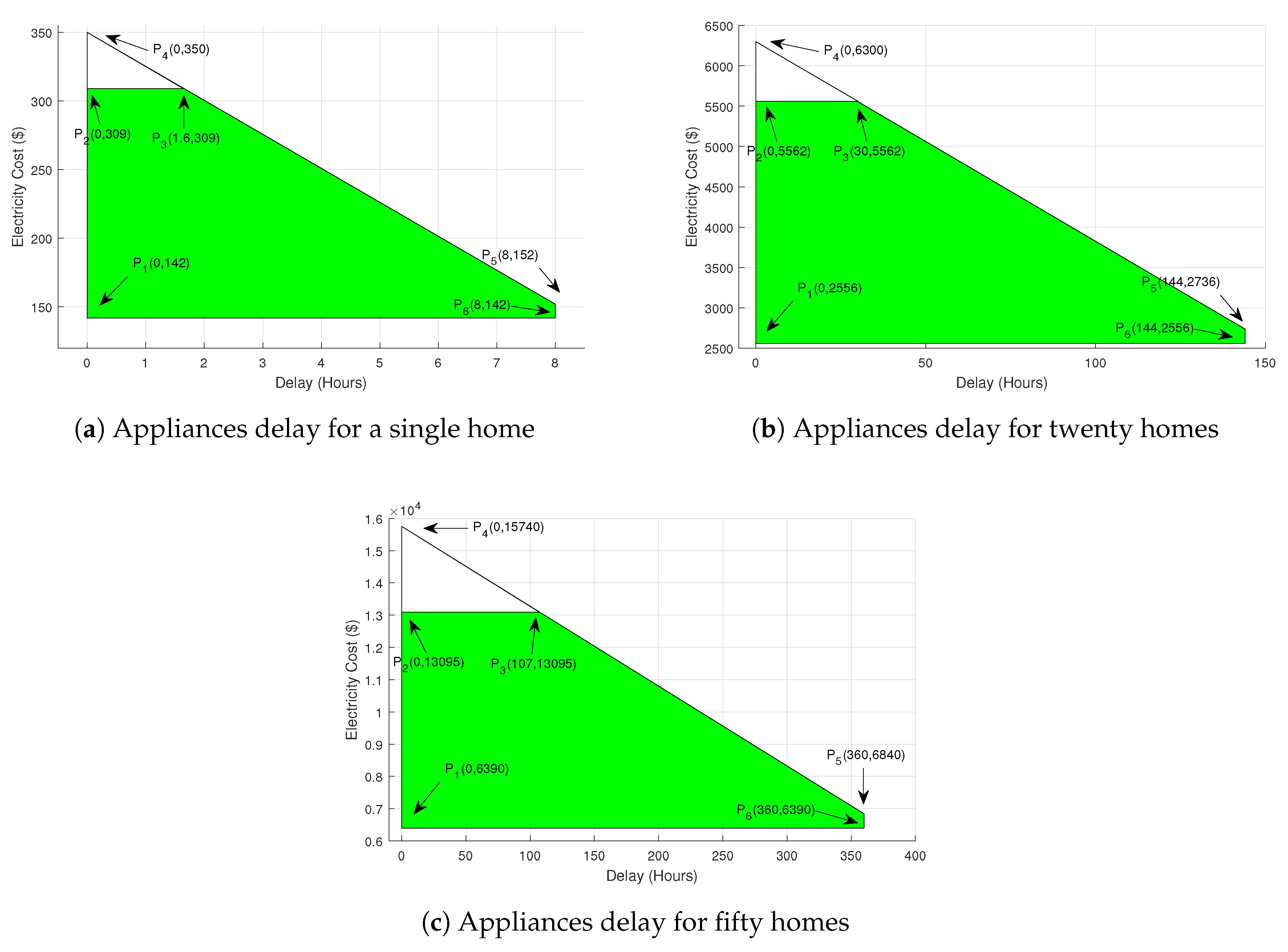
All these appliances must be scheduled from starting time ($t_s$) to finishing time ($t_f$) and maximum delay of 8 h is allowed. The total delay of an appliance can be calculated using Equation (12). Our major objectives are to minimize the cost and maximize the user comfort by minimizing the average waiting time without compromising on PAR. In Equation (18), mathematical expression for PAR is given as:

$$C_t^i=\sum _{t=1}^T\sum _{i=sa}(p_i^r.x_i^t.{\psi }_i^t)$$

(15)

$$Peak=\sum _{t=1}^T\sum _{iϵsa}({p_i}^r).(x_i^t)(\forall t=1\dots 24)$$

(16)

$$Average=1/T\sum _{t=1}^T\sum _{iϵsa}(p_i^r.x_i^t)$$

(17)

$$PAR=Peak/Average$$

(18)

5. System Model

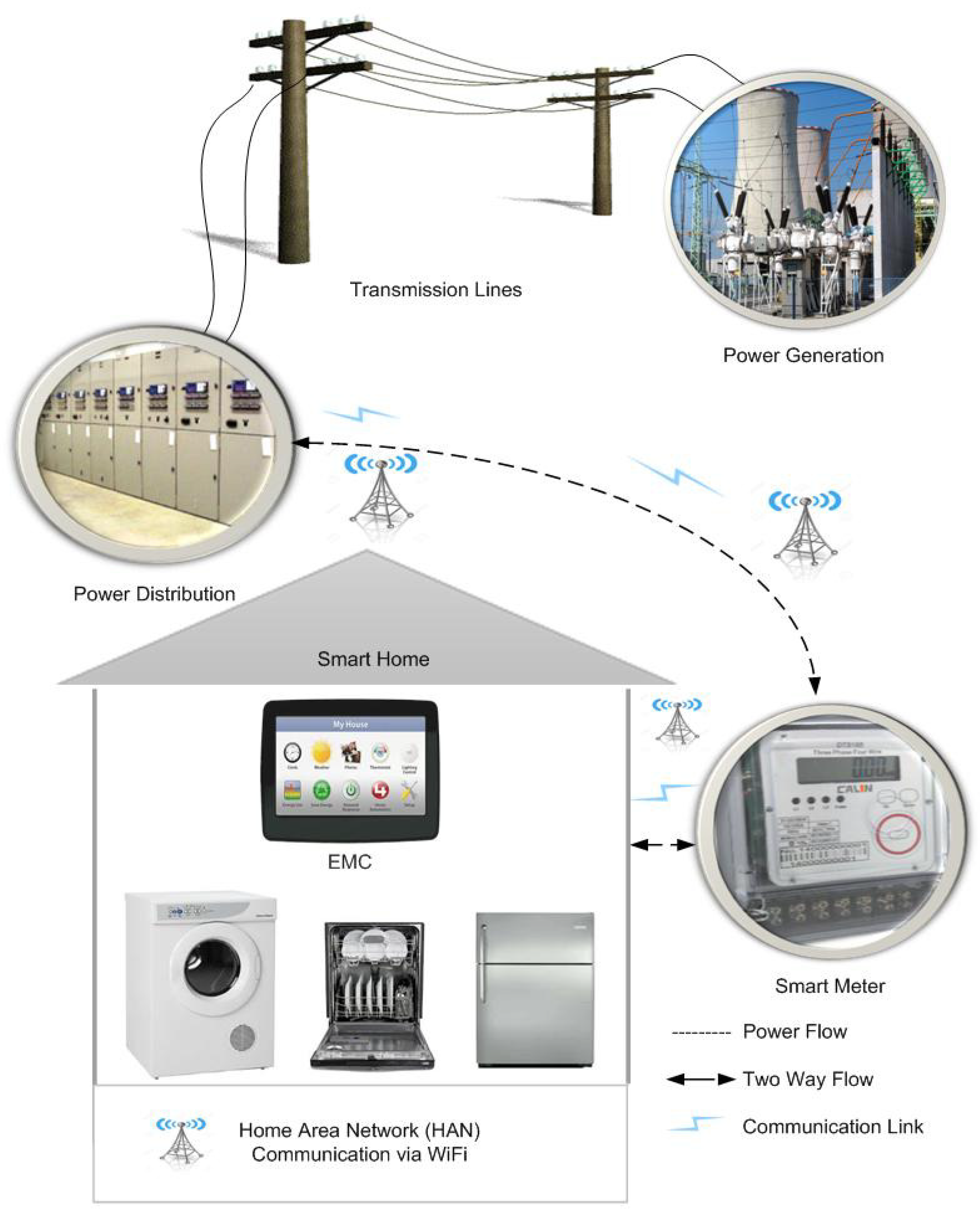
In our proposed model, a smart home consisting of various electrical appliances including washing machine, refrigerator, and cloth dryer etc. A smart meter is installed providing a two-way communication from smart home to the power distribution company. The similar communication takes place between power distribution and transmission. Finally, transmission is connected with power generation with a two way communication link. All appliances are capable to communicate with each other using home area network (HAN) [27,28,29]. The flow of power between the utility and SM is shown by the bold line in Figure 1 and this work is the extension of [5,30]. The communication between EMC, SM and utility is carried out using the wifi or wimax technology. The flow of information between the utility and EMC is bidirectional. We use the DA-RTP and CPP schemes to calculate the electricity cost of multiple homes (single, twenty and fifty homes).

5.1. Day-Ahead Real Time Pricing

Using RTP signals, the massive data flows between the utility and smart home, using DAP an efficient energy consumption scheme is proposed [31]. A wide scope of this strategy is used to tackle the load management problem. In [32], the basic objectives are to improve the system performance and user’s participation in DA-RTP and CPP. However, flat pricing refers to that method, where utility companies charge fix price for all periods. Authors consider flat pricing because price fluctuation is not suited for each consumer, so we optimized the price profile using DA-RTP option. Authors’ basic objective is to make the DA-RTP profile in such a way that the consumer will pay the minimum energy consumption cost by observing the user’s satisfaction.

A DA-RTP model is proposed to resolve the energy management issue between the provider and distribution company by offering optimal DA hourly prices using smart meter. The recent development in the smart metering technologies increases price responsive demands. Several utilities executes a variety of time-based pricing programs; however, most of the utilities used DA-RTP scheme.

In the case of DA-RTP, utilities need to provide planning tools to aid and evaluate the benefits of DA-RTP. The latest example of a system to assist building operator in responding to DA-RTP rates, is the ashere RTP software package which belongs to DA-RTP in the system memory. The basic concept of designing such controller is to help building operator to utilize DA-RTP in an efficient way.

To take advantages from DA-RTP scheme, we require more support system and services. The EMS is able to an automatic scheduling of electricity use under DA-RTP. In this process, EMS requires ongoing monitoring of condition and daily prediction of energy consumption pattern, real time calculation and decision control system. Electricity peak demand makes the power management system unpredictable and peak occurs very infrequently due to which only 20% of the utility side is constructed to handle these peak points.

5.2. Critical Peak Pricing

CPP provides timely information to the consumers about energy cost, specially, during high energy usage periods. This information helps to make more accurate decisions for the efficient utilization energy consumption [33,34]. The CPP provides more accurate information regarding the cost of energy to the consumer, especially, during high energy usage periods, for more accurate decision regarding the electricity consumption. While the price of electricity is higher in CPP events, the CPP rate offers low prices during all other times. This distinction provides a consumer with the opportunity to better assess and potentially reduce your overall annual energy cost.

CPP events mostly occur during an extreme heat wave in summer, extreme cool wave in winter, on Christmas or any other religious event. The CPP events mostly occurred up to four times per year. There is no range of minimum and maximum number of CPP events in a year.San Diego gas and electric (SDGE) has the capability to start CPP events only when it determines the need to call customers for temporary reductions in electricity demand. SDGE notifies to consumers 24 h before the occurrence of event.

6. Proposed Solution

Inspired by the performance of TLBO and EDE, we propose an HT that shifts electric load to OFF peak hours, unburdening ON peak hours. The explanation of the proposed solution is given below in the following subsections.

6.1. Teacher Learning Based Optimization

Evolutionary algorithms adjust their behaviour according to the independent variable that includes population size, crossover percentage and the number of generations. TLBO is inspired by evolutionary algorithms has two main components: learner and teacher. The first component the premature solution that learns from more mature solutions, called teacher [35]. The difference mean is computed as follows.

$$\mathrm{Difference}\mathrm{mean}=r_i(x_{j,kbest,i}-T_f.M_{j,i})$$

(19a)

$$T_f=round[1+Rand(0,1)2-1]$$

(19b)

$$x_{j,k,i}^{\prime }=x_{j,k,i}+(Differenc{e}_{.}{mean)}_{j,k,i}$$

(19c)

In above-mentioned formula, $x_{j,best,i}$ represents the results of best learner in subject j. In Equation (19a), random number is represented by $r_i$ and its value exists with 1 and 2. $T_f$ is a teaching factor whose value varies between 1 and 2 to get the best results. The value of $T_f$ is decided by the formula shown in Equation (19b). $T_f$ is not considered as the parameter of TLBO because its value is calculated randomly. In the above-mentioned expression, $x_{j,k,i}^{\prime }$ is the updated value of $x_{j,k,i}$. This value is accepted if it gives better function value. The second part of the algorithm is related to learner phase where knowledge if another student has more information compared to the current member. Consider a population of size n and two learner P and Q are randomly selected, such that $x_{total-p,i}\ne x_{total-q,i}$ of P and Q, respectively. This equation is used for the minimization problem.

$$x_{j,p,i}^{″}=x_{j,p,i}^{\prime }+r_i(x_{j,p,i}^{\prime }-x_{j,q,i}^{\prime }),if{x}_{total-p,i}^{\prime }\le x_{total-p,i}^{\prime }$$

(19d)

$$x_{j,p,i}^{″}=x_{j,p,i}^{\prime }+r_i(x_{j,q,i}^{\prime }-x_{j,p,i}^{\prime }),if{x}_{total-q,i}^{\prime }\le x_{total-q,i}^{\prime }$$

(19e)

Accept $x_{(j,p,i)}$ when it gives a better function value. All accepted values of the learner phase become the input of teacher phase in the next iteration.

6.2. Enhanced Differential Evolution

Performance of EDE is best compared to DE, the basic reason is that EDE has fewer control parameters as compared to DE. Two basic control parameters based on which DE performance is measured are: population size (NP) and mutant vector (F). The NP and termination criteria is defined in the first step, we choose target vector $x_{i,g}$ from ith vector of the population in current generation, thus we can write it as:

$$x_{i,g}=[x_{1,i,g},x_{2,i,g},x_{3,i,g},\dots ,x_{D,i,g}].$$

(20a)

Target vector is shown by $x_{i,g}$ in Equation (20a). The EDE begins with a population which is randomly initialized between the upper and lower limits within the constraints of search space. In the next step mutation is performed using three vectors $x_{r1,g}$, $x_{r2,g}$ and $x_{r3,g}$ which are selected randomly from target vector. Such that the indexes $r_{1,g}$, $r_{2,g}$ and $r_{3,g}$ are distinct integers. Add the base vector $x_{r1,g}$ to the weighted difference of the vectors $x_{r2,g}$ and $x_{r3,g}$, thus the resultant vector would be the mutant(donor) $v_{i,g+1}$; the mutant vector is presented in Equation (20b) and three groups of NP trial vector are generated by using Equations (20c)–(20e) [36].

$$v_{i,g+1}=x_{r1,g}+F.(x_{r2,g}-x_{r3,g})$$

(20b)

$$\begin{array}{c}\hfill \begin{array}{c}{u}_{j,i,g+1}=\left\{\begin{array}{c}(v_{j,i,g+1})\mathrm{if}\mathrm{randb}(\mathrm{j})\le 0.3\mathrm{or}(j=I_{r}and)\hfill \\ (v_{j,i,g+1})\mathrm{if}\mathrm{randb}(\mathrm{j})\ge 0.3\mathrm{and}(j=I_{r}and)\hfill \end{array}\right.\hfill \end{array}\end{array}$$

(20c)

$$\begin{array}{c}\hfill \begin{array}{c}{u}_{j,i,g+1}=\left\{\begin{array}{c}(v_{j,i,g+1})\mathrm{if}\mathrm{randb}(\mathrm{j})\le 0.6\mathrm{or}(j=I_{r}and)\hfill \\ (v_{j,i,g+1})\mathrm{if}\mathrm{randb}(\mathrm{j})\ge 0.6\mathrm{and}(j=I_{r}and)\hfill \end{array}\right.\hfill \end{array}\end{array}$$

(20d)

$$\begin{array}{c}\hfill \begin{array}{c}{u}_{j,i,g+1}=\left\{\begin{array}{c}(v_{j,i,g+1})\mathrm{if}\mathrm{randb}(\mathrm{j})\le 0.9\mathrm{or}(j=I_{r}and)\hfill \\ (v_{j,i,g+1})\mathrm{if}\mathrm{randb}(\mathrm{j})\ge 0.9\mathrm{and}(j=I_{r}and)\hfill \end{array}\right.\hfill \end{array}\end{array}$$

(20e)

First three groups of trial vectors are obtained using the crossover rate of 0.3, 0.6 and 0.9. Then only one group is selected for the comparison with old populating $x_{i,g}$ in the selection stage. This one group is considered to be the fittest one among three. When a group is selected, in learning period the proposed three groups of the trial vectors are evaluated in every iteration through counter assigned to each group. Finally, the group reaches maximum value, it uses the end of whole set of iteration after the learning period is finished. The best one vector is selected by using Equation (20f)

$$\begin{array}{c}\hfill \begin{array}{c}{x}_{i,g+1}=\left\{\begin{array}{c}(u_{i,g+1})\mathrm{if}(f(u_{i,g+1})\le f(x_{i,g}))\hfill \\ (x_{i,g})\mathrm{otherise}\hfill \end{array}\right.\hfill \end{array}\end{array}$$

(20f)

6.3. Hybrid Technique

We propose an HT that combines the best features of two evolutionary algorithms TLBO and EDE. TLBO is an efficient algorithm in local search, in contrast, EDE performs better for global search. TLBO works better in solution exploitation whereas EDE performs effectively in solution exploration. TLBO, by its nature, is non-parametric whereas EDE has faster convergence rate. Our proposed technique combines the best of the two worlds. Due to the hybridization of the best features of EDE and TLBO, HT shows better convergence rate as compared to EDE and TLBO. The HT procedure is presented in Algorithm 1.

Algorithm 1: HT

Input:  Population Size, crossover Rate, Mutation rate 1: Initialization of parameter 2: Generate population (P, Pop size) 3: Evaluate (P) 4: while (the termination condition is not met)   Teacher phase 5:   $X_{mean}$ = calculate mean vector(P) 6:   $X_{teacher}$ = bset solution(P) 7:   for i = 1...n 8:     TF = round (1+r) 9:     Update solution by selecting the best solution 10:     $X_{new}^i$ = $X_{new}^i$ + rand(0,1) [$X_{teacher}$-($T_f^i$ . $X_{mean}$)] 11:     Objective function 12:     If ($f(X_{new}^i)$ < $f(X^i)$) 13:       $X^i$ = $X_{new}^i$ 14:     end if   Student Phase 15:    Choose different learner $X^j$ s.t $j=i$ 16:     If ($f(X^i)$ < $f(X^j)$) 17:       $X_{new}^i$ = $X^i$ + rand(0,1) ($X^i$ − $X^j$) 18:     else 19:       $X_{new}^i$ = $X^i$ + rand(0,1) ($X^j$ − $X^i$) 20:     end if 21:     If ($f(X_{new}^i)$ < $f(X^i)$) 22:       $X^i$ = $X_{new}^i$ 23:     end if 24:   end for 25:     if (G < = 100) 26:       Perform crossover 27:       Find best member in teacher and learner phase in each itteration 28:       Compare these three crossover function and       Choose the member with least value of objective function 29:     else 30:       Crossover over the current population 31:       In first 100 generations, choose the member with the least value of objective function (the best) 32:     end if 33:     In the search range, run parameter verification 34:     Set G = G + 1 35: end while

7. Results and Discussion

The simulation results are presented in this section and simulations are performed in MATLAB 2017b. We evaluated the each algorithm and selected the best one which satisfies our objective function. To achieve our objectives, we consider three different types of appliances and implemented HT, TLBO [35] and EDE [36]. We assume that electricity price varies between 5 to 20 dollar/kWh. The detailed comparison is provided below.

7.1. Performance Comparison

Three appliances are considered in this work: cloth dryer, refrigerator and dishwasher. The clothes dryer is considered due to the facts that its duty cycles are shorter and has high energy consumption. We analyze the performance of each appliance with respect to cost and delay using two pricing schemes: DA-RTP and CPP. Each appliance has different requirement of energy consumption and time factor.

Table 1. Priorities of appliances.

Appliance	Time Factor	Operational Time (Hour)
Cloth Dryer	1.0 1.5	12
Refrigerator	1.0 1.5	24
Dishwasher	1.0 1.5	9

provides the description of execution time and priorities of the appliances.

• Cloth Dryer
  We consider cloth dryer for scheduling due to its higher flexibility. The performance of cloth dryer is presented in Figure 2a,b. Simulation results for cloth dryer are summarized in

  Table 2. Cloth dryer performance.

  Scheme	Priority	Monthly Cost ($)	Cost Reduction	Average Delay in Hours/Month
  HT	1.5	21.17	45%	3.72
  	1.0	11.76	60%	5.72
  TLBO	1.5	23.20	40%	3.25
  	1.0	15.47	60%	5.42
  EDE	1.5	25.76	33%	2.83
  	1.0	17.71	53%	4.63

  and

  Table 3. Cloth dryer performance (CPP).

  Scheme	Priority	Monthly Cost ($)	Cost Reductiom	Average Delay in Hours/Month
  HT	1.5	22	42%	4.34
  	1.0	14	65%	6.66
  TLBO	1.5	24	37%	4.00
  	1.0	16	58%	5.66
  EDE	1.5	31	28%	3.41
  	1.0	19	50%	5.41

  . In the case of HT, cost is 45% reduced as compared to the unscheduled cost with priority 1.5. By decreasing the appliance priority to 1.0, the cost is further reduced up to 60%. We compare EDE and TLBO with the unscheduled cost; results show that reduction in cost is 33% and 40% with priority 1.5 and show 53% and 60% reduction in the cost when priority is 1.0. However, EDE and TLBO avarage waiting time is 2.83 and 3.25 h, respectively when the priority is 1.0, which is less than the delay time of HT.
  In the second scenario, the same number of appliances is considered with CPP. It reduces the risk of high price in RTP. Simulation results for cost and average waiting time are shown in Figure 3a,b. When CPP signal is used, cloth dryer shows 42% and 65% reduction in cost using HT. TLBO and EDE show 37% and 28% decrease in cost, respectively with the priority of 1.5. When the priority of appliances is reduced to 1.0, TLBO and EDE show reduction in cost 58% and 50%, respectively.
• Refrigerator
  The execution cost and waiting time of refrigerator are illustrated in Figure 4a,b. Simulation results demonstrate that, HT with priority 1.5 reduces cost up to 33% with the average delay of 3.71 h. However, when priority of the refrigerator is 1.0, 62% of cost is reduced with an average delay of 7.71 h.
  Simulation results are summarized in

  Table 4. Refrigerator performance.

  Scheme	Priority	Monthly cost ($)	Cost reduction	Average Delay in Hours/Month
  HT	1.5	402	33%	3.71
  	1.0	225	62%	7.71
  TLBO	1.5	442	26%	3.22
  	1.0	292	51%	6.52
  EDE	1.5	524	12%	2.01
  	1.0	309	48%	5.01

  and

  Table 5. Refrigerator performance (CPP).

  Scheme	Priority	Monthly cost ($)	Cost reduction	Average Delay in Hours/Month
  HT	1.5	420	30%	6.77
  	1.0	252	58%	10.77
  TLBO	1.5	456	25%	6.53
  	1.0	348	41%	8.78
  EDE	1.5	528	11%	5.04
  	1.0	312	47%	8.00

  , which shows that when the priority of refrigerator is 1.5, the TLBO and EDE reduce cost 26% and 12%, respectively.
  If refrigerator is switched ON with the priority of 1.0 then TLBO and EDE reduce the cost up to 51% and 48%, respectively.
  From comparative analysis, it is observed that HT performs better as compared to TLBO and EDE in terms of cost. However, HT have maximum delay as compared to the other heuristic techniques. CPP plays a vital role in demand response electricity markets. Simulation results for cost and average waiting time with cpp are shown in Figure 5a,b, respectively. In RTP, high prices risk can be reduced by utilizing CPP. In the scenario of CPP, the refrigerator shows 30% and 58% reduction in the cost using HT. TLBO and EDE show 25% and 11% reduction in the cost, respectively, with the priority of 1.5.
• Dishwasher
  A dishwasher is an ideal appliance for DSM due to short duty cycles and high energy consumption. Figure 6a,b demonstrate the average waiting time and cost of dishwasher for one month. Simulation results for dishwasher are summarized in

  Table 6. Dishwasher performance.

  Scheme	Priority	Monthly cost ($)	Cost reductiom	Average Delay in Hours/Month
  HT	1.5	56	19%	1.72
  	1.0	36	48%	3.72
  TLBO	1.5	59	15%	1.65
  	1.0	42	40%	3.11
  EDE	1.5	63	10%	1.33
  	1.0	44	37%	2.35

  and

  Table 7. Dishwasher performance (CPP).

  Scheme	Priority	Monthly cost ($)	Cost reductiom	Average Delay in Hours/Month
  HT	1.5	60	14%	2.11
  	1.0	38	45%	4.11
  TLBO	1.5	65	07%	2.02
  	1.0	43	38%	3.77
  EDE	1.5	66	05%	1.45
  	1.0	44	36%	2.75

  . Two-time factors are used for dishwasher, where the large time factor means higher priority and it leads to shorter time. We use four heuristic techniques to find out the best time schedule for a dishwasher at the minimum cost. Simulation results illustrate that HT, TLBO, EDE show 19%, 15% and 10% reduction in cost, with the priority of 1.5. If dishwasher is switched ON at a priority of 1.0 then HT, TLBO, EDE achieve 48%, 40%, 37% reduction in the cost with average delay of 3.72, 3.11, 2.35. By comparing results, we find that the performance of HT is the best in terms of cost and waiting time. If we comparatively see the simulation results then HT shows maximum delay.
  We check the performance of optimization techniques on different appliances by using the CPP signal. Simulation results for dishwasher average waiting time and cost are shown in Figure 7a,b. Simulation results illustrate that HT, TLBO, EDE show 14%, 7%, 5% with an average delay of 2.11, 2.02 and 1.45 h respectively with the priority of 1.5. If priority of the appliance is reduced to 1.0, simulation results illustrate that HT, TLBO and EDE achieved 45%, 38% and 36% reduction in the cost with average delay of 4.11, 3.77 and 2.75 h respectively. HT obtained the best performance in terms of cost; however, the delay is maximized.

7.2. PAR

The best pattern of appliances scheduling is selected where consumer attains minimum cost and maximum user satisfaction for each month. Figure 8 illustrates the PAR using our implemented techniques and unscheduled electricity consumption. Simulation results show that HT achieves minimum peaks as compared to TLBO and EDE and unscheduled PAR using DA-RTP and CPP signals. HT reduces 60% PAR, while TLBO and EDE reduce 50% and 45% PAR, respectively using DA-RTP. In case of CPP, HT achieves minimum PAR, while TLBO and EDE reduce the PAR 48%, 44%, respectively.

7.3. Electricity Consumption

Electricity consumption of appliances depends on power rating and LOT. Figure 9a,b show the monthly electricity consumption schedule of three considered appliances. Simulation results demonstrate that HT reduces peaks as compared to TLBO and EDE. TLBO shows peaks in 2nd and 6th months with 86 kW and 77 kW, with DA-RTP. HT has maximum peak power consumption of 78 kW and 82 kW in 3rd and 7th months. However, HT shows minimum peaks as compared to TLBO and EDE.

Same appliances are considered in the case of CPP. CPP events occurred in 2nd and 6th month. In CPP energy consumption is maximum, different incentives are provided to the consumer to avoid the critical peak events. Simulation results for CPP are shown in Figure 9b. HT shows minimum peak 82 kW and 78 kW kw in 2nd and 6th month respectively. However TLBO and EDE show maximum peak of 92 kW in 2nd and 6th month respectively.

7.4. Scenario 1: Twenty Homes

In our previous section, we consider a single home, however, to tackle the scalability issue, now we implement our proposed scheme for 20 homes. In each home three appliances with different energy consumption stages are considered.

• Cloth Dryer
  We consider the cloth dryer along with both pricing signals (DA-RTP and CPP) and analyze the performance of cloth dryer on the basis of cost and delay of appliance. We measure the performance of cloth dryer for a year and calculate the average for a month. Simulations for cloths dryer energy consumption cost and delay of appliances are shown in Figure 10a,b. By utilizing the DA-RTP signal, optimization techniques HT, TLBO and EDE achieve 33%, 29% and 13% reduction in cost respectively with a priority of 1.5. If we decrease the priority to 1.0 then HT, TLBO and EDE show 65%, 55% and 42% reduction in cost respectively. In the same scenario HT, TLBO and EDE show an average delay of per month respectively with a priority of 1.5. When the priority of appliances is reduced to 1.0 then HT, TLBO and EDE show 114 h, 109 h and 92 h delay of appliances respectively.Simulation results show that there is a tradeoff between the delay of appliances and cost.
  We also conducted simulation by implemented the CPP signal. Simulations result are shown in Figure 11a,b. Simulation results show that HT, TLBO and EDE show 29%, 23% and 12% reduction in cost respectively with a priority of 1.5. When priority is reduced to 1.0 the performance of HT, TLBO and EDE show 60%, 49% and 39% reduction in cost respectively. In our scenario, the critical events occur twice in a year. If we consider the delay of appliances then HT, TLBO and EDE show 93 h, 75 h and 64 h respectively with a priority of 1.5. If the priority is reduced to 1.0 then average delay per month is 122 h, 188 h and 100 h respectively.
• Refrigerator
  We consider refrigerator as a SA because we schedule ice making stage and defrost stage of refrigerator. Scheduling is done for both pricing signal (DA-RTP and CPP). Simulations are shown in Figure 12a,b. When we utilized DA-RTP signal then HT, TLBO and EDE achieve 24%, 17% and 14% reduction in cost respectively with a priority of 1.5 respectively. When the priority of appliance is reduced to 1.0 then HT, TLBO and EDE show 48%, 38% and 35% reduction in cost respectively. In the same scenario HT, TLBO, EDE show an average delay of 217 h, 171 h and 166 h respectively with a priority of 1.0. If these algorithms are considered with a priority of 1.5 then HT, TLBO, EDE show 137 h, 124 h and 106 h respectively. The results show that there is a tradeoff between appliances delay and energy consumption cost.
  In the scenario of CPP, the performance of optimization techniques are different as compared to DA-RTP. Simulations for refrigerator energy consumption cost and delay of appliances are shown in Figure 13a,b. The performance of HT, TLBO and EDE show 24%, 16%, and 13% respectively. If we calculate the delay of refrigerator under the same priority of 1.5 then HT, TLBO and EDE show 145h, 136h, 110h, 90h respectively. when priority is reduced to 1.0 the performance of HT, TLBO and EDE show 47%, 36% and 34% respectively. By reducing the priority we can further save the energy consumption cost.
• Dishwasher
  We divided the energy consumption stages of dishwasher into three parts heated dry, main wash and final rinse. We schedule load among these energy consumption stages in such a way that the consumer will pay the minimum cost. Simulations for dishwasher energy consumption cost and delay of appliances are shown in Figure 14a,b. DA-RTP signal is utilized to find the energy consumption cost by using optimization technique HT, TLBO and EDE show 28%, 21%, 17% reduction in cost respectively with a priority of 1.5. When the priority is reduced to 1.0 then HT, TLBO and EDE show 54%, 48% and 44% reduction in cost respectively. If we consider the dishwasher delay then HT, TLBO and EDE show 35 h, 33 h and 27 h respectively with a priority of 1.5. when the priority of appliances is reduced to 1.0 then HT, TLBO and EDE show 75 h, 63 h and 44 h respectively. CPP signal is also utilized for dishwasher energy consumption scheduling, simulation results for CPP are shown in Figure 15a,b, which show that HT, TLBO and EDE show 43%, 41% and 34% reduction in cost respectively with a priority of 1.5. While priority is reduced to 1.0 the performance of HT, TLBO and EDE is increased up to 83%, 72% and 51%. In our scenario, the critical event occur twice in a year. If we consider the delay of dishwasher then HT, TLBO and EDE show 43 h, 41 h and 34 h respectively with a priority of 1.5. If the priority is reduced to 1.0 then average delay per month increase up to 83 h, 72 h and 51 h respectively.

7.5. Scenario 2: Fifty Homes

In this section, we uncover the results of 50 homes, because our proposed scheme is implemented on small community having 50 homes.

• Cloth Dryer
  The clothes dryer is one of the most energy consuming appliances in the residential sector, but a little work need to be done to schedule its energy consumption stages of clothes dryer in such a way that the consumer will pay the minimum cost. We consider both pricing signal (DA-RTP and CPP) and evaluate the performance of cloth dryer on the basis of cost and delay of appliances. We measure the performance of cloths dryer for a year and calculate the average for a month. Simulations for cloths dryer energy consumption cost and delay of appliances are shown in Figure 16a,b. By utilizing the DA-RTP signal, optimization techniques HT, TLBO and EDE show 45%, 37% and 31% reduction in cost respectively with a priority of 1.5. If we decrease the priority to 1.0 then HT, TLBO, EDE reduce cost up to 67%, 57% and 52% reduction in cost respectively. In the same scenario HT, TLBO and EDE show an average delay of 75 h, 65 h and 56 h per month respectively with a priority of 1.5. When the priority of appliances is reduced to 1.0 then HT, TLBO, EDE show delay of appliances 114 h, 109 h and 92 h respectively. Simulation results evaluation show that there is a tradeoff between the delay of appliances and cost.
  CPP signal is also implemented in our scenario and conducted the simulation, simulations are shown in Figure 17a,b. Results show that HT, TLBO and EDE obtained 43%, 34% and 25% reduction in cost respectively with a priority of 1.5. While priority is reduced to 1.0 the performance of HT, TLBO and EDE increase up till to 66%, 56% and 48% respectively. If we consider the delay of appliances then HT, TLBO and EDE show 93 h, 75 h and 64 h respectively with a priority of 1.5. If the priority is reduced to 1.0 then average delay per month is 122 h, 188 h and 100 h, respectively.
• Refrigerator Simulations of refrigerator with 50 homes are shown in Figure 18a,b. When we utilized DA-RTP signal then HT, TLBO and EDE show 28%, 21% and 20% reduction in cost respectively with a priority of 1.5 respectively. When the priority of appliance is reduced to 1.0 then HT, TLBO and EDE show 50%, 44% and 43% reduction in cost respectively. In the same scenario HT, TLBO and EDE show an average delay of 217 h, 171 h and 166 h respectively with a priority of 1.0. If these algorithms are considered with a priority of 1.5 then HT, TLBO and EDE show 137 h, 124 h and 106 h respectively. The results show that there is a tradeoff between appliances delay and energy consumption cost.
  When we implement the CPP, the performance of optimization technique is different as compared to DA-RTP. Simulations for Refrigerator energy consumption cost and delay of appliances are shown in Figure 19a,b. The performance of HT, TLBO and EDE show 25%, 18% and 15% reduction in cost respectively. In the case when priority is reduced to 1.0 the performance of HT, TLBO and EDE show 47%, 36% and 34% respectively. If we calculated the delay of refrigerator then HT, TLBO and EDE show 145 h, 136 h, 110 h respectively with a priority of 1.5. By reducing the priority we can further save the energy consumption cost.
• Dishwasher
  A dishwasher act as an integrated more permanent kitchen appliances. It has large load capacity as compared to other most of the home appliances. Simulations for dishwasher electricity cost and delay of an appliance are shown in Figure 20a,b. In DA-RTP signal HT, TLBO and EDE show 35%, 24% and 27% reduction in cost respectively with a priority of 1.5. When the priority is reduced to 1.0, The optimization techniques HT, TLBO and EDE show 62%, 49% and 51% reduction in cost respectively. If we consider the dishwasher delay then HT, TLBO and EDE show 35 h, 33 h and 27 h respectively with a priority of 1.5. HT, TLBO, EDE show 75 h, 63 h and 44 h respectively, with reduced priority 1.0.
  Simulation are also conducted for CPP and simulation results are shown in Figure 21a,b, which show that HT, TLBO and EDE show 31%, 21% and 20% reduction in cost respectively with a priority of 1.5. While priority is reduced to 1.0 the performance of HT, TLBO and EDE show 60%, 48% and 45%. If we consider the delay of appliances then HT, TLBO and EDE show 43 h, 41 h and 34 h respectively with a priority of 1.5. If the priority is reduced to 1.0 then average delay per month is 83 h, 72 h and 51 h respectively.

7.6. Performance Tradeoff

Results show a tradeoff between appliances delay and energy consumption cost. In all the scenario of single and multiple homes optimization techniques reduce the energy consumption cost and as well as appliances delay at minimum level. Appliances delay greatly effect by energy consumption cost and it cause a reduction in cost. Relationship between energy consumption cost and appliances delay are shown in Figure 22a.

Table 8. Performance Tradeoff.

Scheme	Monthly cost ($)	Cost reduction	Average Delay in Hours/Month
HT	21.17	45%	3.72
TLBO	23.20	40%	3.25
EDE	25.76	33%	2.83

shows a performance tradeoff between energy consumption cost and appliances delay. The electricity cost waiting time are minimized by existing optimization techniques such as TLBO. However HT performing well in terms of minimize energy consumption at the cost of maximum delay of the appliance.

8. Feasible Region

A area which contains logical and real possible solutions of any problems considered feasible region. The feasible regions of our work are expressed below.

8.1. Feasible Region for Energy Consumption Cost

Pictorial representation of feasible region is shown in Figure 23a. An area under these points $P_1$(0.17, 52), $P_2$(8.2, 500), $P_3$(10, 600), $P_4$(10, 500), $P_5$(10, 300) and $P_7$(0.17, 0.14) is a feasible region for power consumption. In the given region $P_3$(10, 600) is a maximum extreme where maximum cost can occur. A threshold for the given cost at point $P_2$ and $P_4$ are shown by a straight line, $P_2$(8.2, 500) and $P_4$(10, 500) represent the maximum cost at which appliance are used for a specific time slot. $P_3$(10, 600) and $P_5$(10, 300) show the maximum and minimum energy consumption cost when maximum load is being operated at a minimum and maximum cost. $P_2$(8.2, 500) show the maximum cost when energy consumption load is 8.1. The line connecting $P_4$ and $P_5$ represent that the consumer can reduce their energy consumption cost by shifting appliances from on peak hours to off-peak hours. Similarly, $P_2$(8.2, 500) and $P_4$(10, 500) depict same energy consumption cost.

Scalability issue is managed by considering twenty and fifty homes and calculate the electricity cost of appliances in term of power consumption. In this scenario, our objective function also remains same but the number of homes is increased. Pictorial representation of feasible region is shown in Figure 23b. Feasible region is actually the area enclosed by points $P_1$(3.4, 1040), $P_2$(164, 10,000), $P_3$(200, 12,000), $P_4$(200, 6000), $P_5$(164, 5000) and $P_6$(3.4, 280). The maximum energy consumption cost at any point must not exceed 5465. This is actually the threshold which is calculated for energy consumption cost. $P_1$(4440, 162) is the maximum energy consumption cost at minimum load and $P_6$(3.4, 280) is minimum energy consumption cost at minimum load. $P_2$(4440, 162) and $P_4$(4440, 200) represent the same energy consumption cost but the use of energy is different for different cost. $P_4$(200, 6000) and $P_5$(164, 5000) depict the same use of energy at minimum cost 78 dollar and maximum cost 222 dollar. We can say that as the use of energy consumption increased the cost of energy is also increased so these are directly proportional.

In the scenario of 50 homes, energy consumption cost is calculated by using the same objective function. Graphical view of feasible region is shown in Figure 23c. Feasible region is actually the area enclosed by points $P_1$(7, 650), $P_2$(380, 25,000), $P_3$(450, 29,500), $P_4$(450, 25,000), $P_5$(450, 13,500) and $P_6$(7, 26). $P_6$(7,26) and $P_1$(7,650) represent the minimum and maximum power consumption at a minimum and maximum cost and the maximum cost of an appliance can utilize is the $P_2$(380, 25,000). At point $P_2$(380, 25,000) and $P_4$(450, 25,000) energy, consumption cost is the same however different power is consumed. $P_4$ and $P_5$ show the same energy consumption cost however the electricity cost is different at both points.

8.2. Feasible Region for Delay of Appliances

There is an inverse relationship between the delay of an appliance and electricity cost. Feasible region for delay of appliances is shown in Figure 22a. This feasible region demonstrate the electricity cost for a year. Point $P_1$(0,142) shows that user cannot bear any delay for appliances and pays the minimum cost and $P_4$(0, 350) shows the minimum delay at maximum cost. $P_5$(8, 152) shows maximum delay at minimum cost and $P_6$(8, 142) shows the maximum delay at minimum cost and $P_3$(0, 309) and $P_4$(1.6, 309) shows the maximum threshold for the electricity cost. This demonstrates the minimum energy consumption cost paid by user by shifting appliance to low price hours.

Electricity cost and appliance’s delay are inverse to each other. Pictorial representation of feasible region is shown in Figure 22b. By increasing the cost, appliances delay are reduced at a minimum level and at zero delay consumer will pay maximum electricity cost. $P_1$(0, 2556) represents the zero delay and maximum cost. $P_4$(0, 6300) shows the zero delay at maximum cost. we find a Nash equilibrium between energy consumption cost and appliances delay in such a way that the consumer will pay the minimum energy consumption cost. $P_5$(144, 2736) shows the maximum delay at maximum cost and $P_6$(144, 2556) shows the maximum delay at minimum cost. We draw a threshold for electricity cost, which is not more than 5562 dollar. This shows that suitable appliances can save a reasonable amount of energy by compressing the energy demand and schedule an appliance in off peak hour.

A tradeoff exists between the electricity cost and the delay of an appliance. Pictorial representation of feasible region for a year is shown in Figure 22c. By increasing the delay of an appliance the consumer will pay the minimum energy consumption cost. $P_1$(0, 6390) represents the zero delay at minimum cost and $P_4$(0, 15,740) shows the minimum delay at maximum cost. $P_5$(360, 6840) and $P_6$(360, 6390) shows the maximum delay at maximum cost and maximum delay at minimum cost respectively. $P_2$(0, 13,095) and $P_3$(107, 13,095) show the threshold for electricity consumption cost. This shows that suitable appliances can save a reasonable amount of energy by compressing the energy demand and schedule an appliance to off peak hour.

9. Conclusions

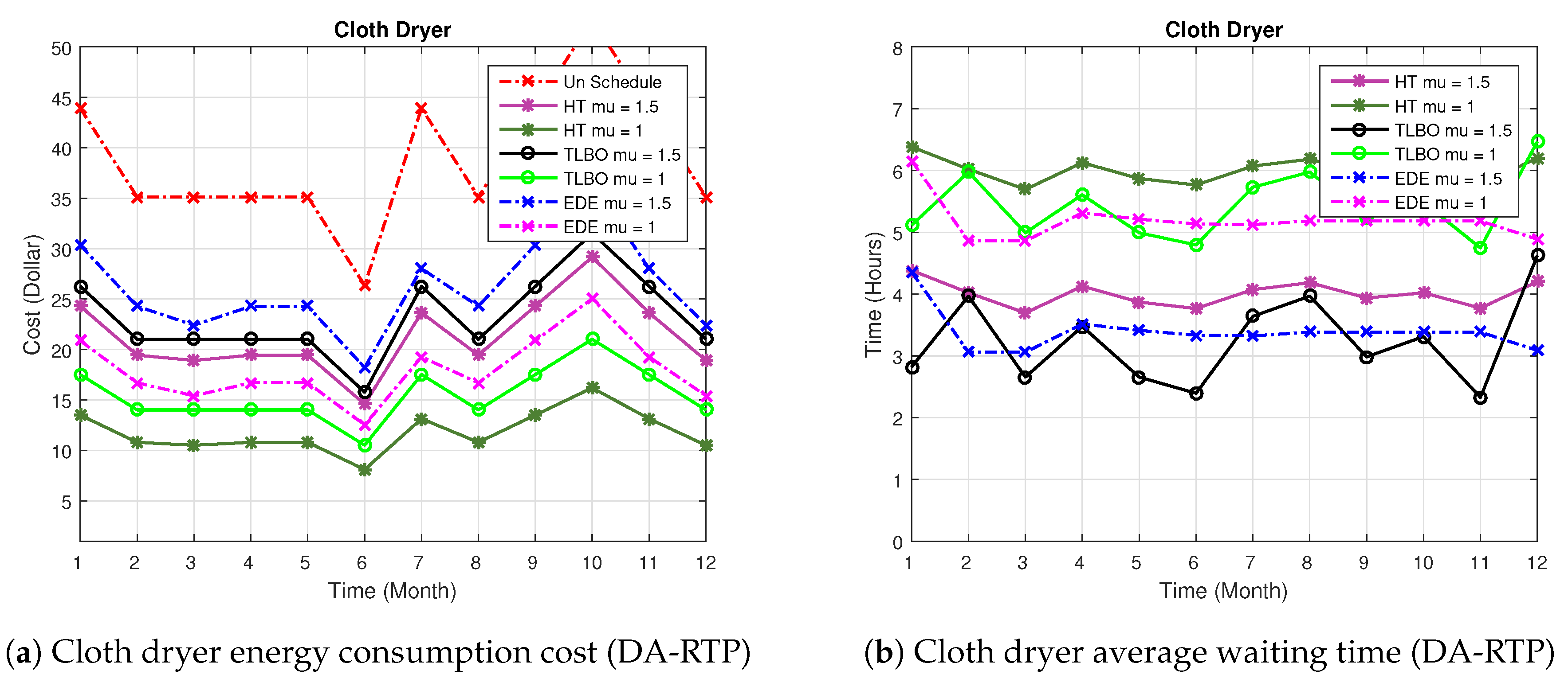
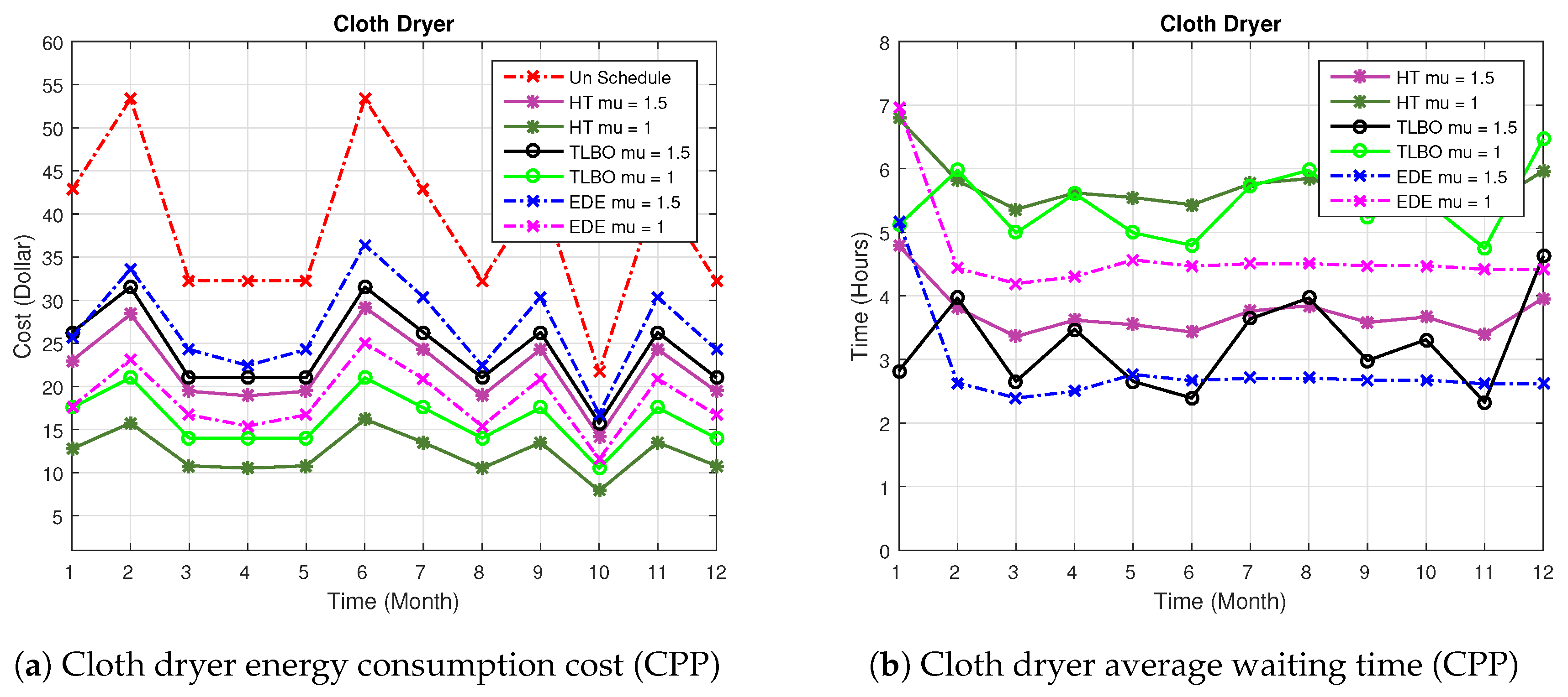
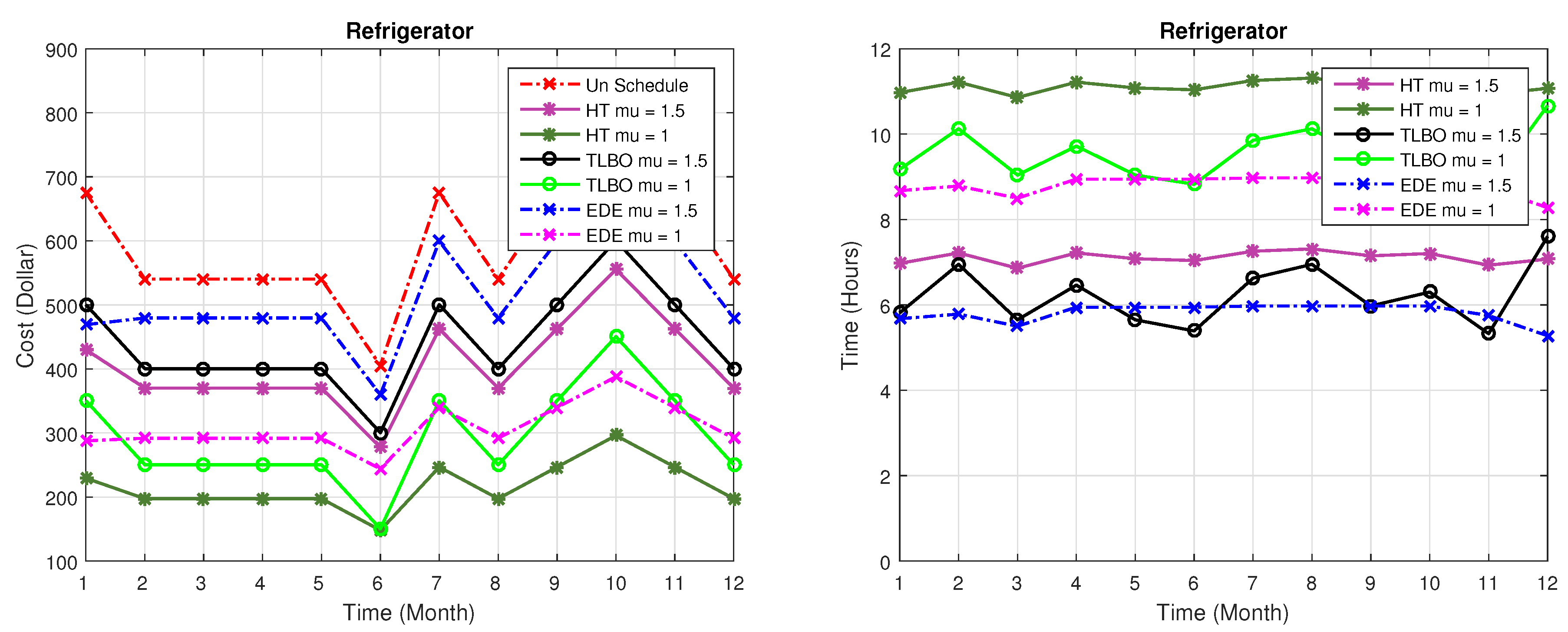
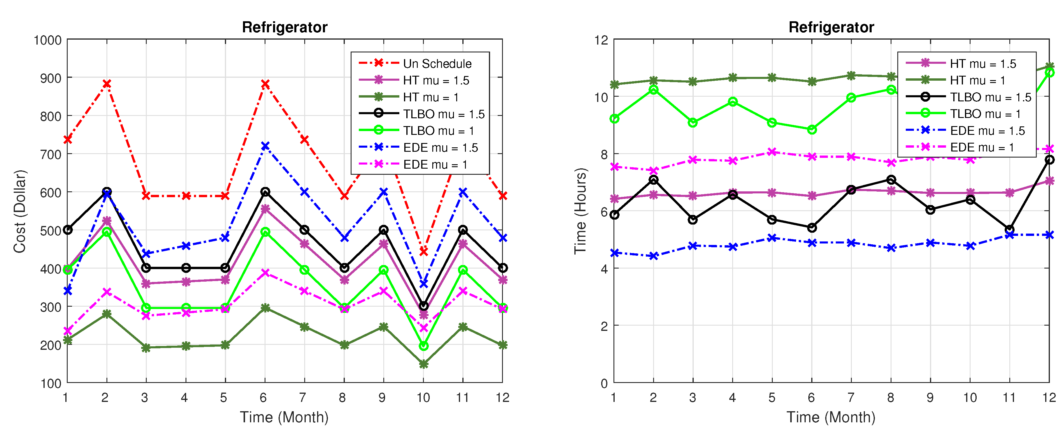
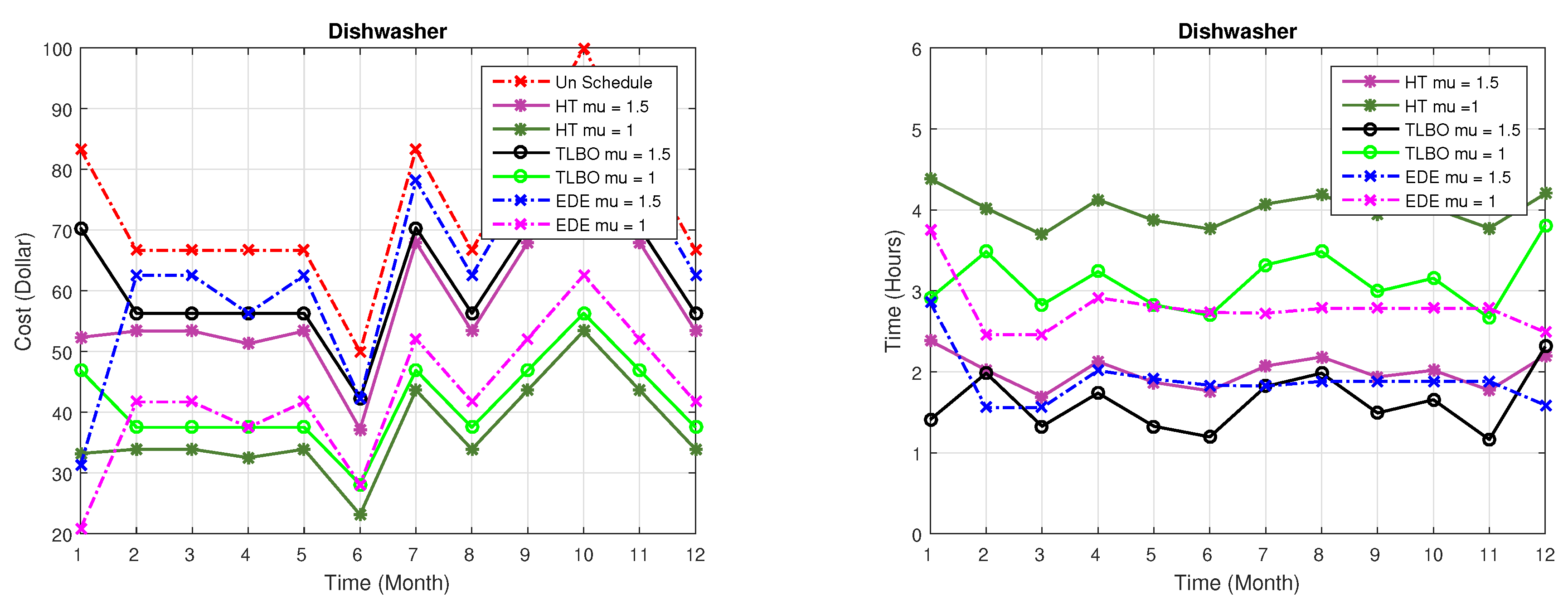
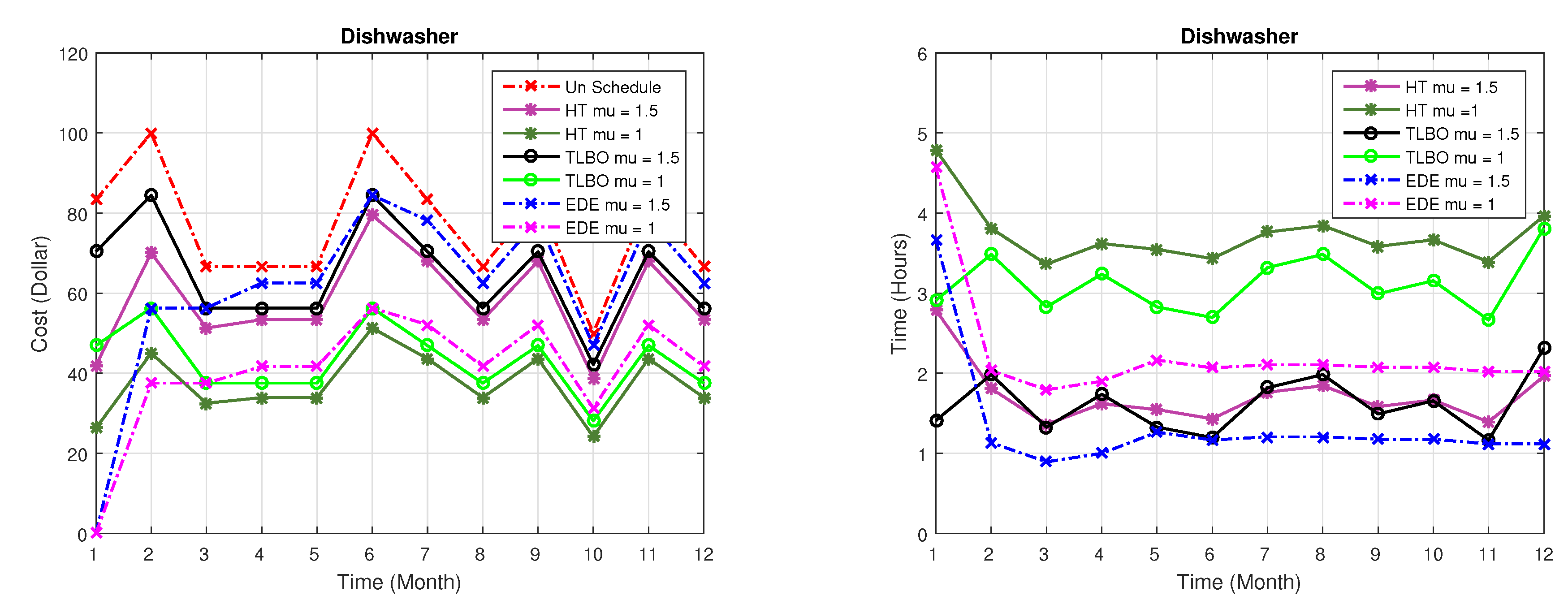
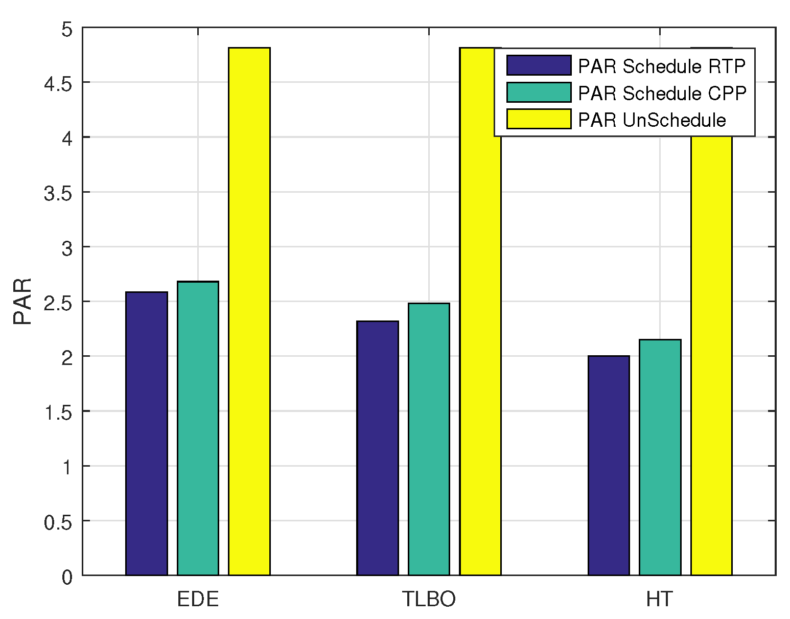
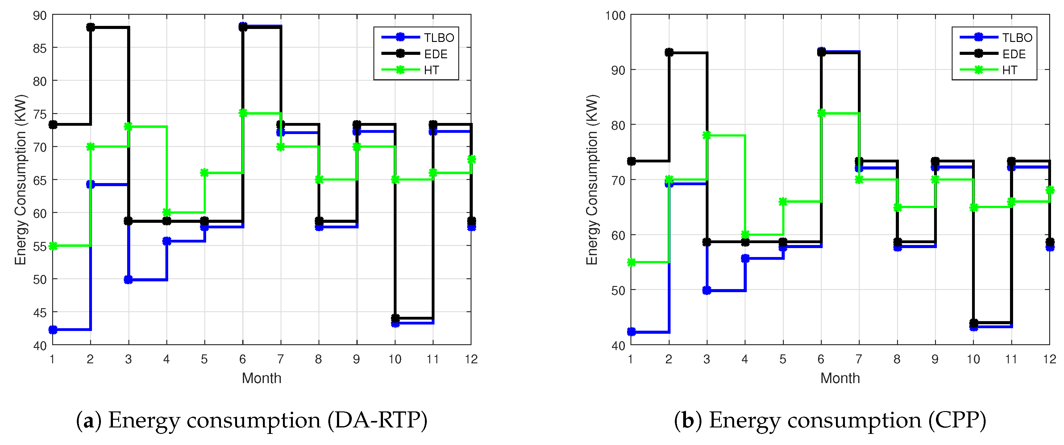
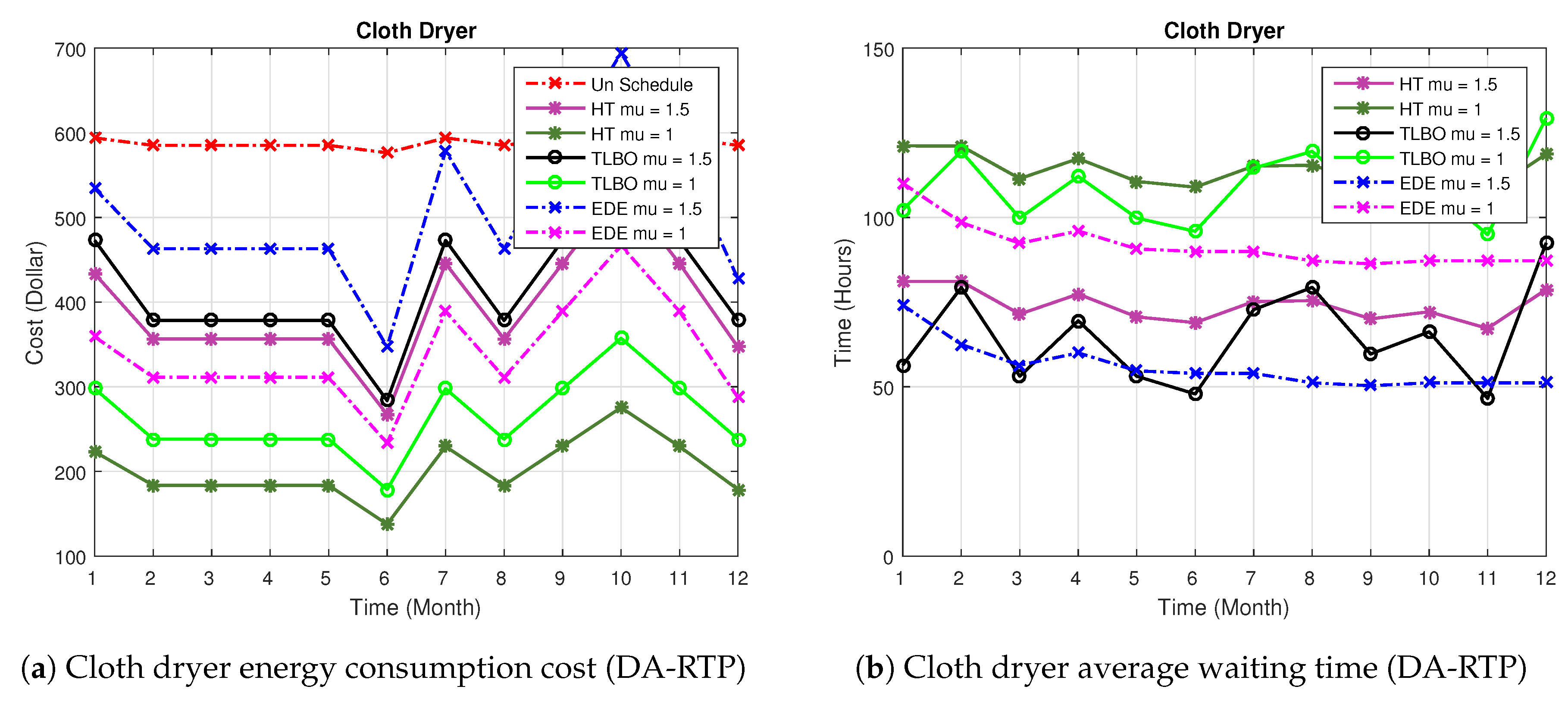
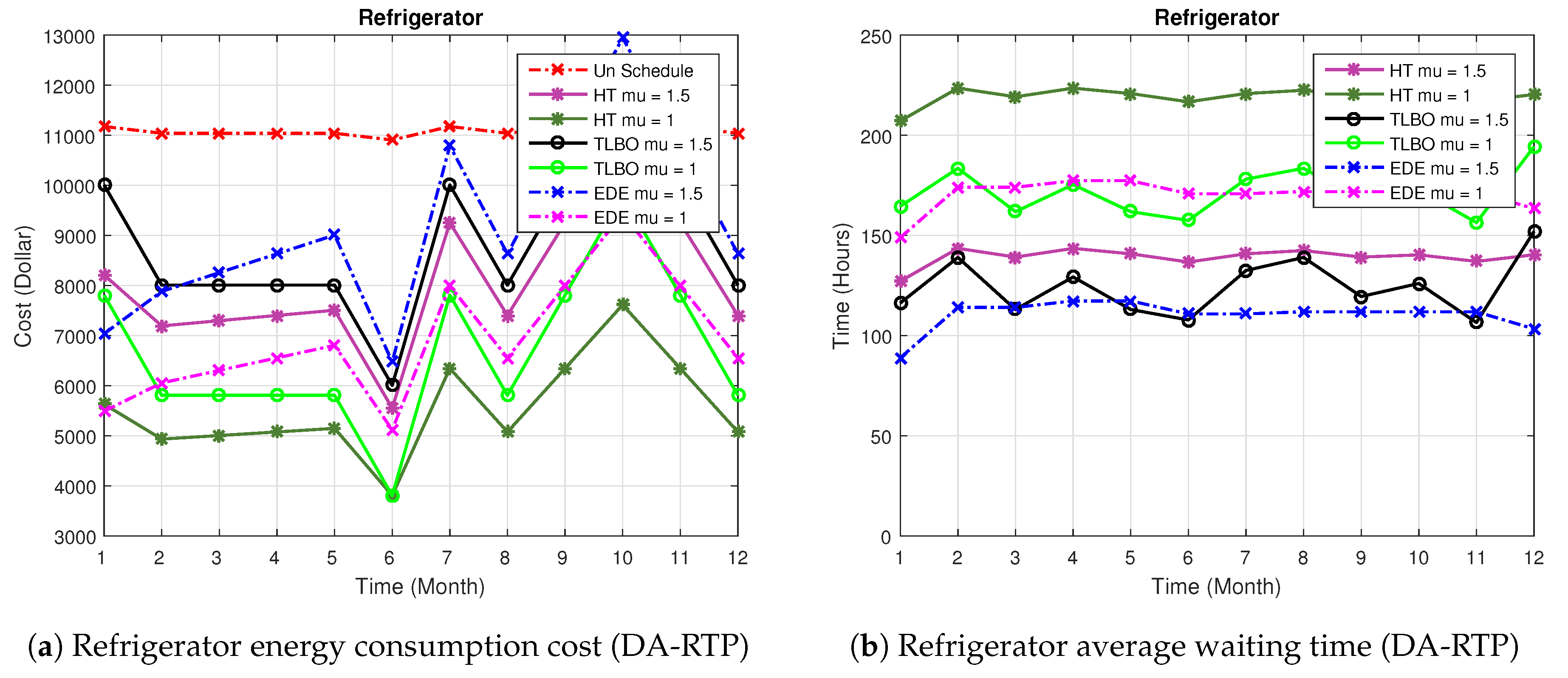
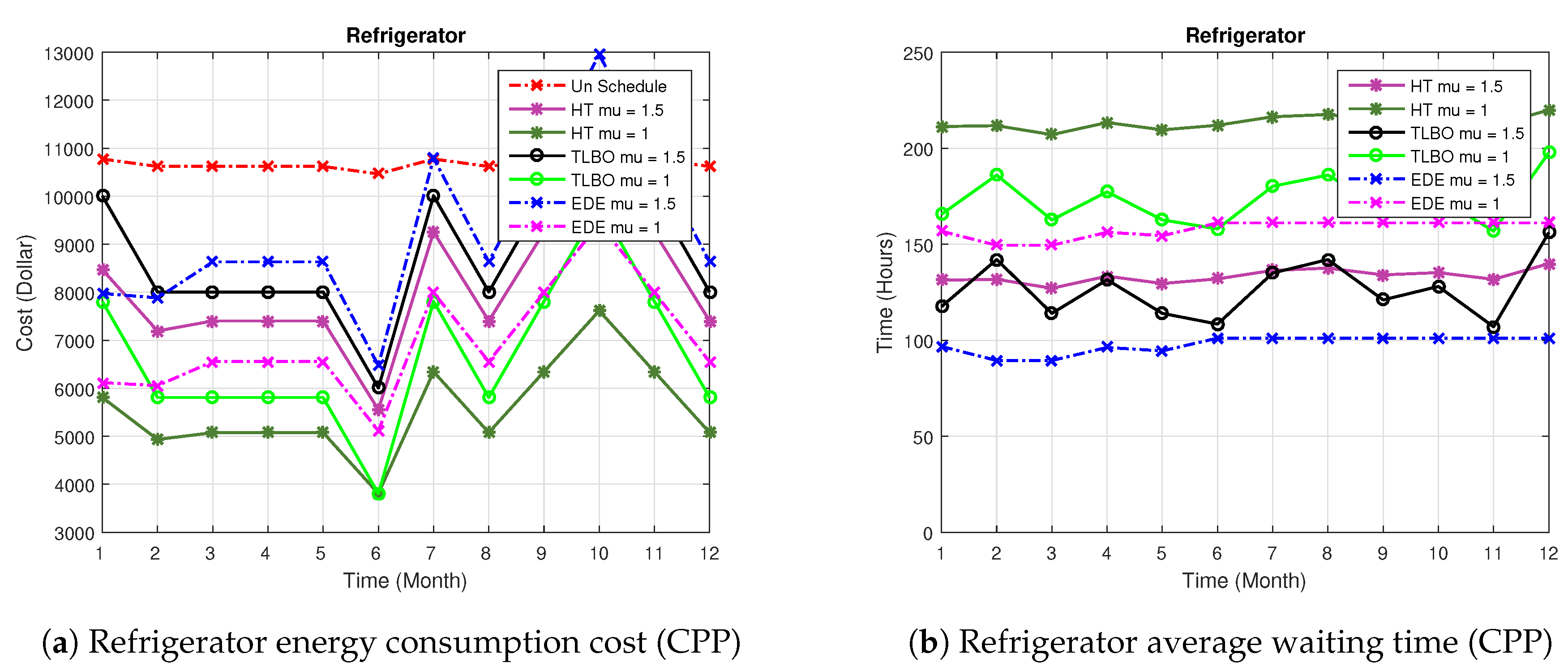
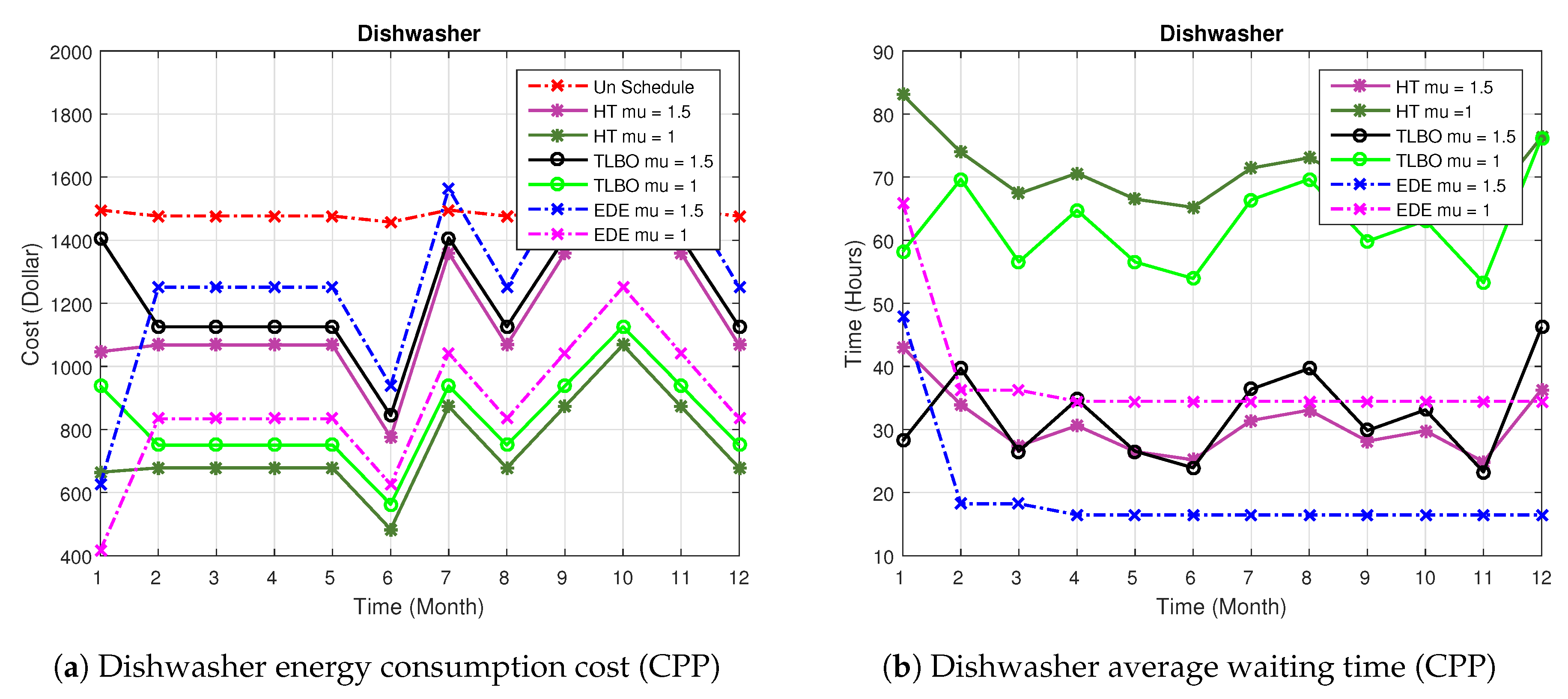
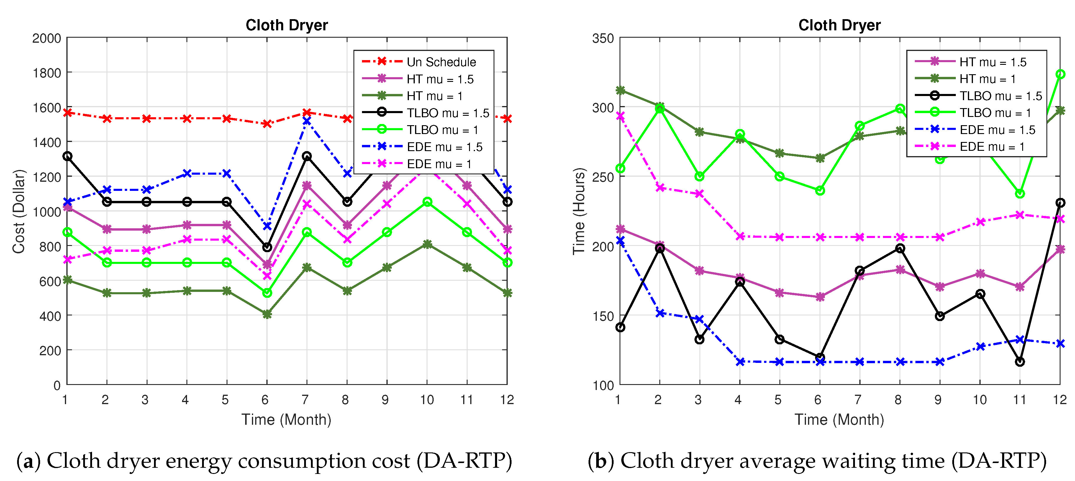
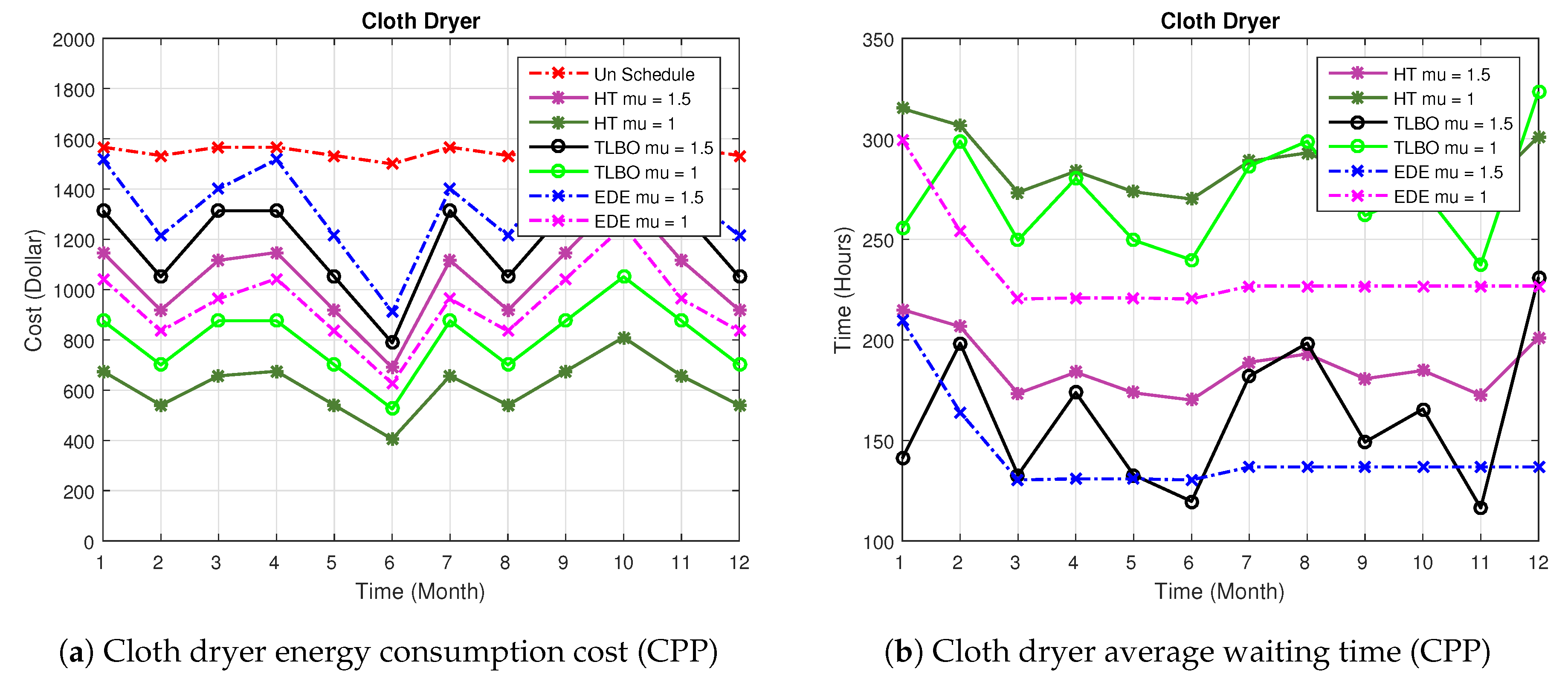
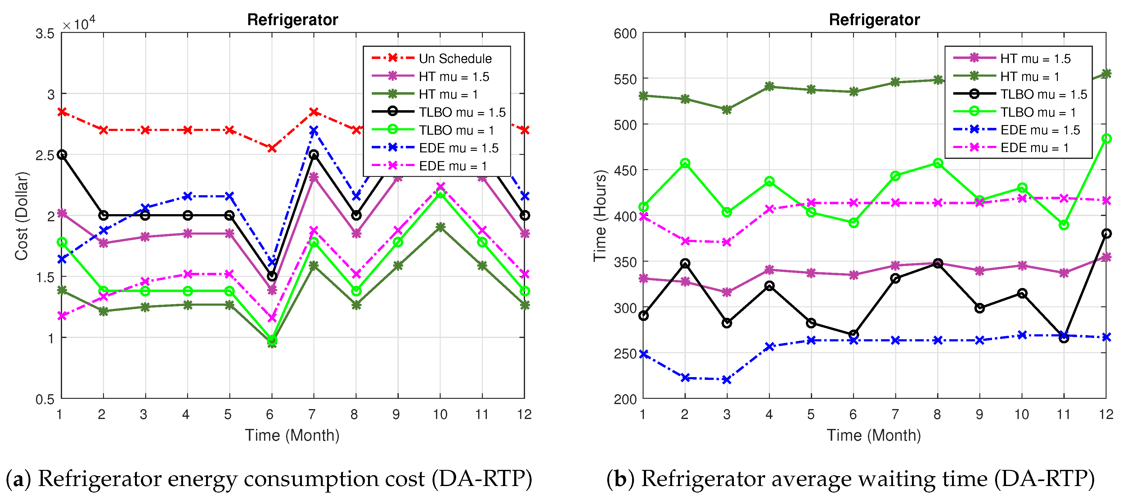
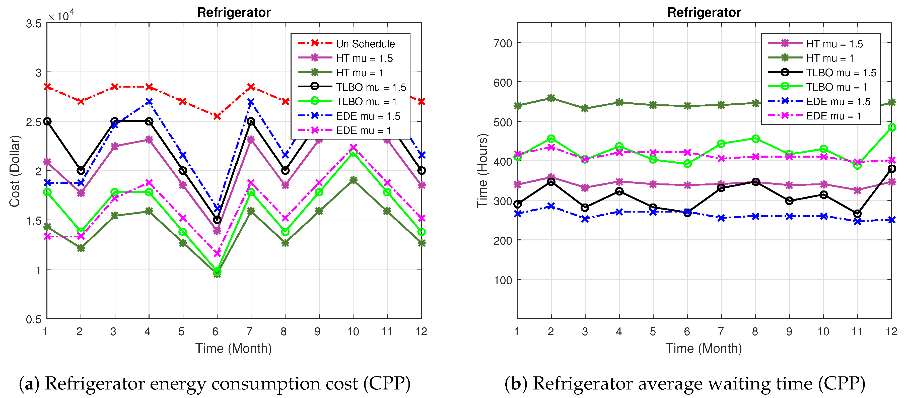
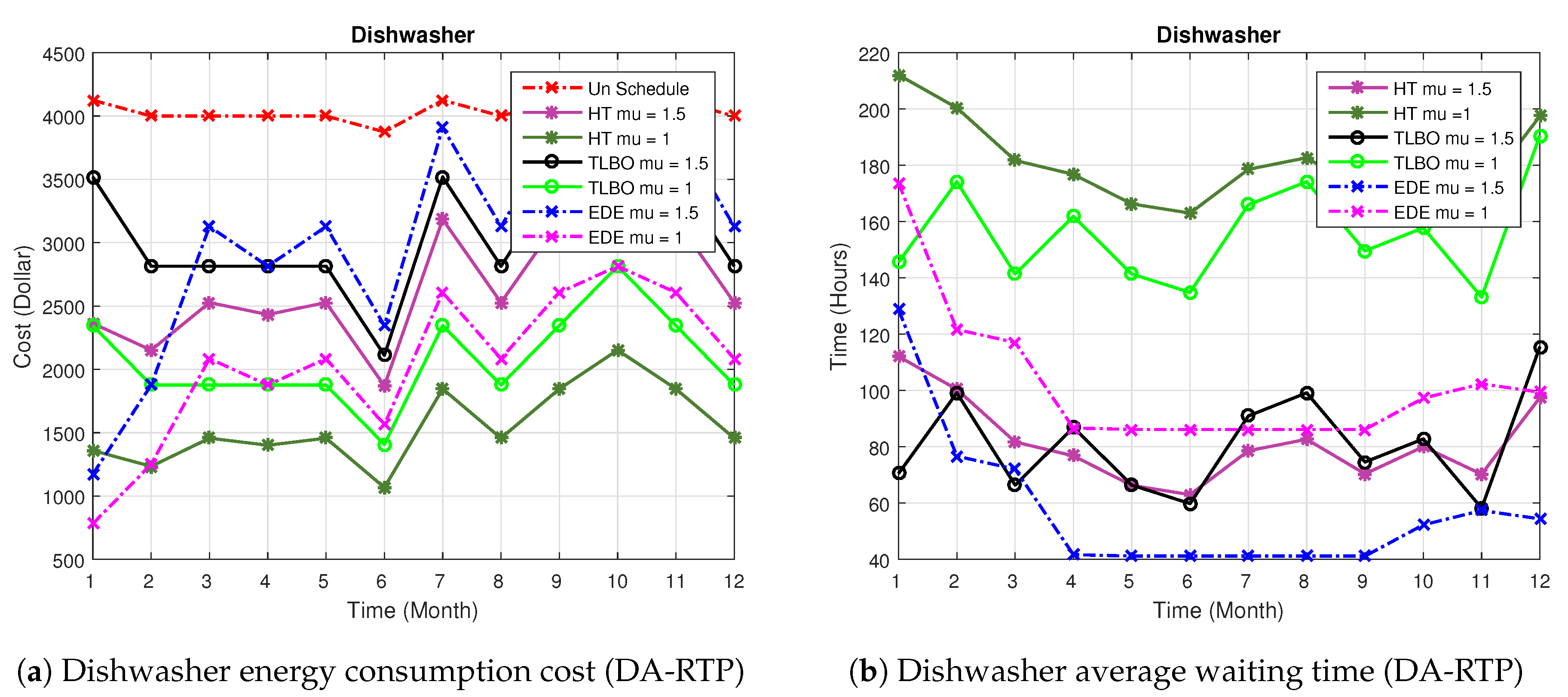
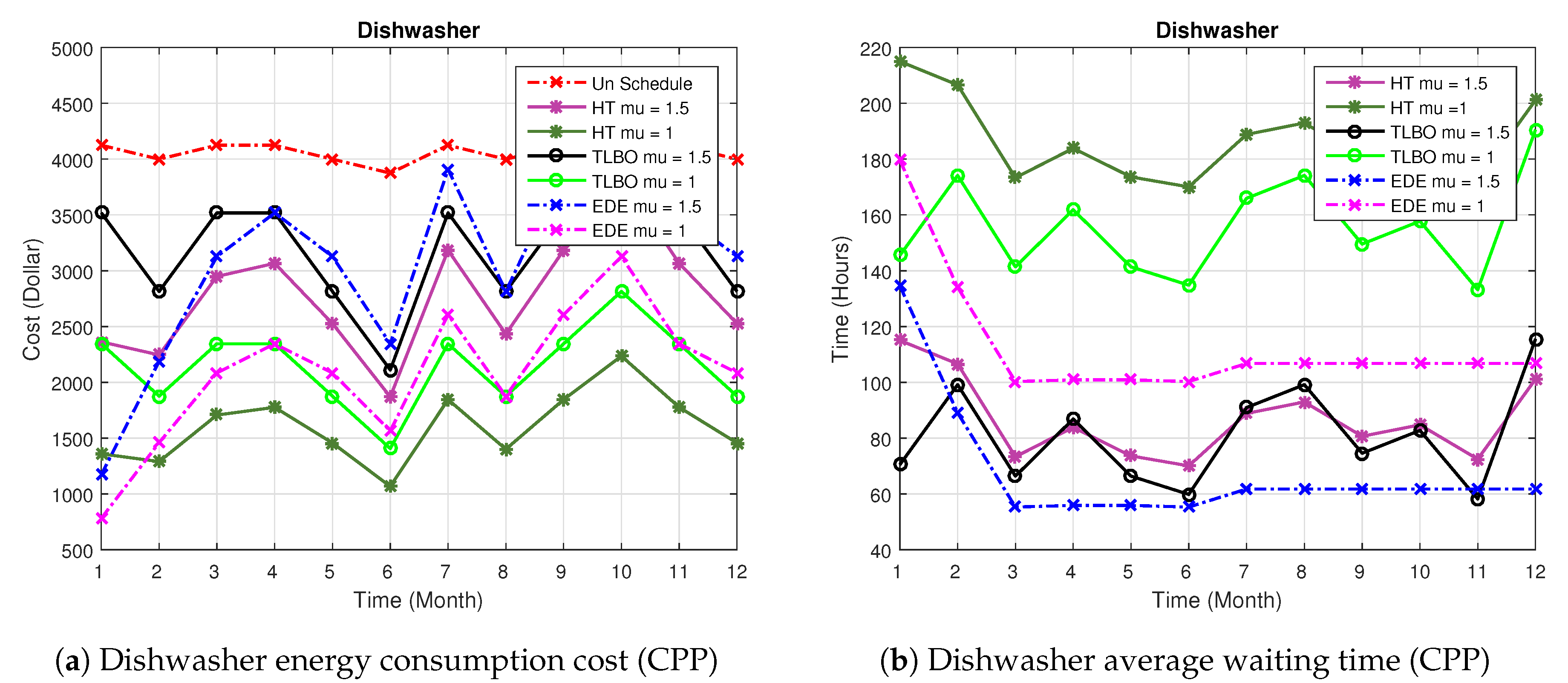
DSM has the potential to provide lot of advantages to the entire smart grid, particularly at distribution network level. In this work, we have proposed a DSM scheme for electricity cost and PAR minimization with maximum consumers’ satisfaction. For comparative analysis, existing algorithms TLBO and EDE are implemented in our optimization problem with the same parameters. We have tested the proposed scheme on multiple smart homes with the objective to schedule the smart appliances where consumer pays less electricity cost along with maximum satisfaction level and minimum PAR. To validate the proposed scheme, extensive simulations are conducted against the parameters of PAR, electricity expenses and average waiting time. It is evident from the results that proposed HT scheme outperforms existing techniques with minimum cost, waiting time and PAR. Moreover, the monthly electricity cost of HT, TLBO and EDE is reduced by 45%, 40% and 39%, respectively. Additionally, significant reduction is observed on average PAR which is 58%, 52% and 48% of HT, TLBO and EDE, respectively.

References

1. Howell, S.; Rezgui, Y.; Hippolyte, J.L.; Jayan, B.; Li, H. Towards the next generation of smart grids: Semantic and holonic multi-agent management of distributed energy resources. Renew. Sustain. Energy Rev. 2017, 77, 193–214. [Google Scholar] [CrossRef]
2. Pasetti, M.; Rinaldi, S.; Manerba, D. A Virtual Power Plant Architecture for the Demand-Side Management of Smart Prosumers. Appl. Sci. 2018, 8, 432. [Google Scholar] [CrossRef]
3. Gellings, C.W. The Concept of Demand-Side Management for Electric Utilities. Proc. IEEE 1985, 73, 1468–1470. [Google Scholar] [CrossRef]
4. Ghazvini, M.A.F.; Soares, J.; Abrishambaf, O.; Castro, R.; Vale, Z. Demand response implementation in smart households. Energy Build. 2017, 143, 129–148. [Google Scholar] [CrossRef]
5. Ahmed, A.; Manzoor, A.; Khan, A.; Zeb, A.; Madni, H.A.; Qasim, U.; Khan, Z.A.; Javaid, N. Performance Measurement of Energy Management Controller Using Heuristic Techniques. In Conference on Complex, Intelligent, and Software Intensive Systems; Springer: Cham, Switzerland, 2017; pp. 181–188. [Google Scholar]
6. Zhang, Q.; Wang, X.; Fu, M. Optimal implementation strategies for critical peak pricing. In Proceedings of the 2009 6th International Conference on the European Energy Market (EEM 2009), Leuven, Belgium, 27–29 May 2009; pp. 1–6. [Google Scholar]
7. Khan, A.R.; Mahmood, A.; Safdar, A.; Khan, Z.A.; Khan, N.A. Load forecasting, dynamic pricing and DSM in smart grid: A review. Renew. Sustain. Energy Rev. 2016, 54, 1311–1322. [Google Scholar] [CrossRef]
8. Aslam, S.; Iqbal, Z.; Javaid, N.; Khan, Z.A.; Aurangzeb, K.; Haider, S.I. Towards Efficient Energy Management of Smart Buildings Exploiting Heuristic Optimization with Real Time and Critical Peak Pricing Schemes. Energies 2017, 10, 2065. [Google Scholar] [CrossRef]
9. Mitra, K.; Dutta, G. Electricity Consumption Scheduling with Energy Storage, Home-Based Renewable Energy Production and A Customized Dynamic Pricing Scheme; No. WP 2016-11-01; Indian Institute of Management Ahmedabad, Research and Publication Department: Ahmedabad, India, 2016. [Google Scholar]
10. Gupta, I.; Anandini, G.N.; Gupta, M. An hour wise device scheduling approach for demand side management in smart grid using particle swarm optimization. In Proceedings of the 2016 National Power Systems Conference (NPSC), Bhubaneswar, India, 19–21 December 2016; pp. 1–6. [Google Scholar]
11. Ahmed, N.; Levorato, M.; Li, G.-P. Residential Consumer-Centric Demand Side Management. IEEE Trans. Smart Grid 2017. [Google Scholar] [CrossRef]
12. Li, C.; Yu, X.; Yu, W.; Chen, G.; Wang, J. Efficient computation for sparse load shifting in demand side management. IEEE Trans. Smart Grid 2017, 8, 250–261. [Google Scholar] [CrossRef]
13. Nguyen, H.K.; Song, J.B.; Han, Z. Distributed demand side management with energy storage in smart grid. IEEE Trans. Parallel Distrib. Syst. 2015, 26, 3346–3357. [Google Scholar] [CrossRef]
14. Bharathi, C.; Rekha, D.; Vijayakumar, V. Genetic Algorithm Based Demand Side Management for Smart Grid. Wirel. Pers. Commun. 2017, 93, 481–502. [Google Scholar] [CrossRef]
15. Arif, A.; Javed, F.; Arshad, N. Integrating renewables economic dispatch with demand side management in micro-grids: A genetic algorithm-based approach. Energy Effic. 2014, 7, 271–284. [Google Scholar] [CrossRef]
16. Pampara, G.; Engelbrecht, A.P.; Franken, N. Binary differential evolution. In Proceedings of the 2016 IEEE Congress on Evolutionary Computation (CEC 2006), Vancouver, BC, Canada, 16–21 July 2006; pp. 1873–1879. [Google Scholar]
17. Zazo, J.; Zazo, S.; Macua, S.V. Robust Worst-Case Analysis of Demand-Side Management in Smart Grids. IEEE Trans. Smart Grid 2017, 8, 662–673. [Google Scholar] [CrossRef]
18. Atzeni, I.; Ordóñez, L.G.; Scutari, G.; Palomar, D.P.; Fonollosa, J.R. Demand-side management via distributed energy generation and storage optimization. IEEE Trans. Smart Grid 2013, 4, 866–876. [Google Scholar] [CrossRef]
19. Moon, S.; Lee, J.-W. Multi-Residential Demand Response Scheduling with Multi-Class Appliances in Smart Grid. IEEE Trans. Smart Grid 2016. [Google Scholar] [CrossRef]
20. Vardakas, J.S.; Zorba, N.; Verikoukis, C.V. Power demand control scenarios for smart grid applications with finite number of appliances. Appl. Energy 2016, 162, 83–98. [Google Scholar] [CrossRef] [Green Version]
21. Brahman, F.; Honarmand, M.; Jadid, S. Optimal electrical and thermal energy management of a residential energy hub, integrating demand response and energy storage system. Energy Build. 2015, 90, 65–75. [Google Scholar] [CrossRef]
22. Pedrasa, M.A.A.; Spooner, T.D.; MacGill, I.F. Coordinated scheduling of residential distributed energy resources to optimize smart home energy services. IEEE Trans. Smart Grid 2010, 1, 134–143. [Google Scholar] [CrossRef]
23. Khomami, H.P.; Javidi, M.H. An efficient home energy management system for automated residential demand response. In Proceedings of the 2013 13th International Conference on Environment and Electrical Engineering (EEEIC), Wroclaw, Poland, 1–3 November 2013; pp. 307–312. [Google Scholar]
24. Bozchalui, M.C.; Hashmi, A.A.; Hassen, H.; Cañizares, C.A.; Bhattacharya, K. Optimal operation of residential energy hubs in smart grids. IEEE Trans. Smart Grid 2012, 3, 1755–1766. [Google Scholar] [CrossRef]
25. Hussain, H.M.; Javaid, N.; Iqbal, S.; Ul Hasan, Q.; Aurangzeb, K.; Alhussein, M. An Efficient Demand Side Management System with a New Optimized Home Energy Management Controller in Smart Grid. Energies 2018, 11, 190. [Google Scholar] [CrossRef]
26. Ma, K.; Yao, T.; Yang, J.; Guan, X. Residential power scheduling for demand response in smart grid. Int. J. Electr. Power Energy Syst. 2016, 78, 320–325. [Google Scholar] [CrossRef]
27. Depuru, S.S.S.R.; Wang, L.; Dev-abhaktuni, V. Smart meters for power grid: Challenges, issues, advantages and status. Renew. Sustain. Energy Rev. 2011, 15, 2736–2742. [Google Scholar] [CrossRef]
28. Man, K.L.; Yue, Y.; Lu, C.; Huang, Q. System design, analysis and optimization of Li-Fi based energy harvesting embedded systems for “Internet of Things” applications. In Proceedings of the International Conference on Internet of Things and Convergence, Jeju Island, Korea, 28–30 October 2015; pp. 189–192. [Google Scholar]
29. Huang, Q.; Li, X.; Shaurette, M.; Cox, R.F. Novel Sensor Network Architecture for Intelligent Building Environment Monitoring and Management. In Proceedings of the 2011 Computing in Civil Engineering, Miami, FL, USA, 19–22 June 2011; pp. 347–354. [Google Scholar]
30. Ahmed, A.; Rahim, M.H.; Feroze, F.; Zafar, A.; Fatima, I.; Aslam, S.; Javaid, N. Swarm Intelligence Based Home Energy Management Controller Under Dynamic Pricing Scheme. In Proceedings of the International Conference on Broadband and Wireless Computing, Communication and Applications, Barcelona, Spain, 8–10 November 2017; Springer: Cham, Switzerland, 2017; pp. 256–266. [Google Scholar]
31. Vardakas, J.S.; Zorba, N.; Verikoukis, C.V. A survey on demand response programs in smart grids: Pricing methods and optimization algorithms. IEEE Commun. Surv. Tutor. 2015, 17, 152–178. [Google Scholar] [CrossRef]
32. Li, Z.; Huang, H.; Zang, C.; Yu, H. Day-ahead real-time pricing strategy based on the price-time-type elasticity of demand. In Proceedings of the 2013 15th IEEE International Conference on Communication Technology (ICCT), Guilin, China, 17–19 November 2013; pp. 449–455. [Google Scholar]
33. Strengers, Y. Peak electricity demand and social practice theories: Reframing the role of change agents in the energy sector. Energy Policy 2012, 44, 226–234. [Google Scholar] [CrossRef]
34. Su, W.; Huang, A.Q. Proposing a electricity market framework for the Energy Internet. In Proceedings of the Power and Energy Society General Meeting (PES), Vancouver, BC, Canada, 21–25 July 2013; pp. 1–5. [Google Scholar]
35. Rao, R. Review of applications of TLBO algorithm and a tutorial for beginners to solve the unconstrained and constrained optimization problems. Decis. Sci. Lett. 2016, 5, 1–30. [Google Scholar]
36. Arafa, M.; Sallam, E.A.; Fahmy, M.M. An enhanced differential evolution optimization algorithm. In Proceedings of the 2014 Fourth International Conference on Digital Information and Communication Technology and It’s Applications (DICTAP), Bangkok, Thailand, 6–8 May 2014; pp. 216–225. [Google Scholar]
Figure 1. Components of DSM.
Energies 11 01464 g001
Figure 2. Electricity cost and waiting time of cloth dryer with (DA-RTP).
Energies 11 01464 g002
Figure 3. Electricity cost and waiting time of cloth dryer with (CPP).
Energies 11 01464 g003
Figure 4. Refrigerator waiting time and electricity cost with (DA-RTP).
Energies 11 01464 g004
Figure 5. Refrigerator energy consumption cost and waiting time with (CPP).
Energies 11 01464 g005
Figure 6. Dishwasher waiting time and electricity cost with (DA-RTP).
Energies 11 01464 g006
Figure 7. Dishwasher energy consumption cost and waiting time with (CPP) .
Energies 11 01464 g007
Figure 8. PAR.
Energies 11 01464 g008
Figure 9. Energy consumption profile.
Energies 11 01464 g009
Figure 10. Scenario 1: Cloth dryer behavior with (DA-RTP).
Energies 11 01464 g010
Figure 11. Scenario 1: Cloth dryer behavior with (CPP).
Energies 11 01464 g011
Figure 12. Scenario 1: Refrigerator behavior with (DA-RTP).
Energies 11 01464 g012
Figure 13. Scenario 1: Refrigerator behavior with (CPP).
Energies 11 01464 g013
Figure 14. Scenario 1: Dishwasher behavior with (DA-RTP).
Energies 11 01464 g014
Figure 15. Scenario 1: Dishwasher behavior with (CPP).
Energies 11 01464 g015
Figure 16. Scenario 2: Cloth dryer behavior with (DA-RTP).
Energies 11 01464 g016
Figure 17. Scenario 2: Cloth dryer behavior with (CPP).
Energies 11 01464 g017
Figure 18. Scenario 2: Refrigerator behavior with (DA-RTP).
Energies 11 01464 g018
Figure 19. Scenario 2: Refrigerator behavior with (CPP).
Energies 11 01464 g019
Figure 20. Scenario 2: Dishwasher behavior with (DA-RTP).
Energies 11 01464 g020
Figure 21. Scenario 2: Dishwasher behavior with (CPP).
Energies 11 01464 g021
Figure 22. Feasible region of waiting time.
Energies 11 01464 g022
Figure 23. Feasible region of energy consumption.
Energies 11 01464 g023