Methodology for Extracting Potential Customized Bus Routes Based on Bus Smart Card Data


School of Traffic and Transportation, Beijing Jiaotong University, Beijing 100044, China
*
Author to whom correspondence should be addressed.
Energies 2018, 11(9), 2224; https://0-doi-org.brum.beds.ac.uk/10.3390/en11092224
Submission received: 1 July 2018
/
Revised: 15 August 2018
/
Accepted: 22 August 2018
/
Published: 24 August 2018
Abstract
:To alleviate traffic congestion and traffic-related environmental pollution caused by the increasing numbers of private cars, public transport (PT) is highly recommended to travelers. However, there is an obvious contradiction between the diversification of travel demands and simplification of PT service. Customized bus (CB), as an innovative supplementary mode of PT service, aims to provide demand-responsive and direct transit service to travelers with similar travel demands. But how to obtain accurate travel demands? It is passive and limited to conducting online surveys, additionally inefficient and costly to investigate all the origin-destinations (ODs) aimlessly. This paper proposes a methodological framework of extracting potential CB routes from bus smart card data to provide references for CB planners to conduct purposeful and effective investigations. The framework consists of three processes: trip reconstruction, OD area division and CB route extraction. In the OD area division process, a novel two-step division model is built to divide bus stops into different areas. In the CB route extraction process, two spatial-temporal clustering procedures and one length constraint are implemented to cluster similar trips together. An improved density-based spatial clustering of application with noise (DBSCAN) algorithm is used to complete these procedures. In addition, a case study in Beijing is conducted to demonstrate the effectiveness of the proposed methodological framework and the resulting analysis provides useful references to CB planners in Beijing.
1. Introduction
With the rapid economic development, hyper-motorization and expanding urban areas have contributed to various traffic-related problems, including traffic congestion, degraded levels of transit, traffic fatalities and injuries, and serious environmental pollution. To effectively mitigate such adverse effects, an efficient, reliable, and reasonable-priced public transport (PT) system is urgently needed [1,2]. The traditional PT service as well as a series of related policies do solve these traffic-related problems more or less, whereas the more and more diverse and characteristic travel demands of travelers are increasingly not being satisfied. In recent years, the development of information and tele-communication technology provides the possibility to build an integrated information sharing platform for transit operators and users. A new innovative mode of public transport services, called customized bus (CB), has been launched and implemented successfully [3].
The most distinctive feature of CB is customization. Passengers specify travel requests with their origins, destinations, and desired pickup or delivery times through interactive online information platforms, such as the Internet, telephones and smartphone apps. Then, the CB operator aggregates similar travel demands and publishes candidate bus routes for users to reserve seats, so CB is a demand-responsive transit system. Users participate in various planning activities and have a great influence on the eventually launched CB routes. Different from conventional bus transport systems, the aim of which is to serve majority of the travelers, CB provides advanced, attractive, and user-oriented service to specific passenger groups with similar travel demands, especially commuters [4]. The CB service is an innovative transport service between conventional buses and taxis in terms of the degree of user participation in operational planning activities, the level of services, and operating cost. CB system generally provides direct and one person one seat transit services, which have no or very few immediate stops as well as multiple stops in the origin and destination areas. Meanwhile, it has the characteristics of fixed stops, fixed vehicles, fixed timetables, fixed prices, fixed passengers, yet flexible route segments. In view of these characteristics, the ticket price of customized buses is more expensive than that of conventional buses, but cheaper than taxis. With the advantages of traffic congestion reduction, traffic safety improvement, better travel experience, and environmental friendliness, the CB system is actively promoted and has become very popular in more and more cities around the world, such as Beijing and Lisbon [4,5,6].
Since customized buses are a new successful public transport mode, the existing regulations and models for conventional buses, e.g., [1,2,7], are not suitable for the CB system. Scientific and systematic methodologies for CB policy making, planning programming, operation and dispatch must be carried out. So far, scholars have conducted a great many studies of this burgeoning service. Liu, et al. provided a systematic analysis of CB practice, elaborated the steps and suggestions for planning and management and measured the operational performance compared with other travel modes [3,4]. Chang and Schonfeld compared this flexible route subscription bus system with fixed route conventional buses [8]. Potts, et al. provided a guide for planning and operating flexible transport services [9]. Vine, et al. used a general framework to forecast the market potential and impacts of carsharing systems [10]. Lorimier and El-Geneidy sought to find the determine factors affecting vehicle usage [11]. However all the aforementioned studies just concentrate on theoretical analysis rather than specific methods.
In 2017, Ma, et al. proposed a methodological framework, including large-scale travel demand data processing, CB line OD area division, CB line OD area pairing, and a line selection model, for CB network design [12], but the travel demands, the basis of network planning, used in the paper were collected through an online survey. This is a passive approach for both the planners and operators and it suffers the following problems: (1) The dataset is unilateral and limited as it only contains the travel demands of certain passengers who participate in the survey; (2) the accuracy and reliability of data cannot be guaranteed because of the arbitrariness and low threshold of participating in this survey; (3) it becomes changeless once the users submit their travel demands, which may result in the increase of invalid data; (4) it is very tedious, inefficient, and costly to plan CB routes by analyzing the survey data manually. Therefore, discovering similar travel demands and planning CB routes more reliably and cost-efficiently is a popular topic [13].
Traffic big data availability has brought significant changes to urban intelligent transportation systems. As an important component of traffic big data, bus smart card data (SCD) plays an irreplaceable role in urban public transport systems because of its wide coverage, high reliability, easy accessibility, and low cost [14]. In this paper, a “from point to line” framework for route extraction is proposed by analyzing trip characteristics based on the bus SCD. Specifically, this framework includes three parts. First, trips are reconstructed from the transaction records of the bus SCD. Then, all the bus stops are divided into several traffic areas by a two-step division model, in which the adopted radiuses are different according to the spatial distribution features of bus stops. Lastly, similar trips are gathered together to generate a large amount of trip flows, of which the regularity are further investigated to identify regular routes. The route length constraint must be satisfied at the same time to extract potential CB routes. Models of last two parts are described in detail and the framework is employed in a case study in Beijing. The result of this research provides a method of extracting potential CB routes and helps CB operators conduct purposeful and effective surveys or investigations.
The remainder of this paper is organized as follows: Section 2 first presents a general overview of the entire framework and emphasizes the two major processes conducted in this study. Section 3 then provides the details of methodology about how to divide origin-destination (OD) areas and extract CB routes using the reconstructed trips, followed by an experiment conducted in Beijing to illustrate the framework in Section 4. The paper concludes by summarizing the research of findings and suggesting directions for future research in Section 5.
2. Framework Description
This section explains the main ideas of the complete framework, including the purpose of each process. Generally speaking, the framework consists of three parts: trip reconstruction, origin-destination (OD) area division and CB route extraction. A flow chart of the framework is illustrated in Figure 1.
A perfect smart card transaction would contain user smart card ID, bus line ID, boarding and alighting stops and times, riding date, etc., but because of the charging purpose of Automatic Fare Collection (AFC) systems [14], the data directly produced from AFC is incomplete. The complete and essential information must be obtained using a number of appropriate methods from bus SCD records, bus GPS data and schedule tables if necessary, as well as some static databases, such as bus stop information and bus line information. Trips, including one or several transactions, must be reconstructed by identifying transfer behaviors from the successive transactions of each user. A series of studies have been done to process the data obtained from AFC system, to infer origin and destination locations, and to estimate transfer points. Chapleau and Chu proposed a multistep method to identify and revise incorrect or suspicious observations and provide suitable origin-destination travel data [15]. Trépanier et al. built a model to estimate the alighting location for passengers who only need to be validated when boarding [16]. Munizaga and Palma presented a methodology for building public transport OD matrices from SCD and GPS data [17]. The mentioned methods are really just the tip of the iceberg, please see Pelletier et al. [14] for a detailed literature review. Due to the various types of AFC systems, the bus SCD structures in different systems are not uniform, targeted method must be used depending on the specific data structure. In view of the existence of numerous related references, the process of trip reconstruction will not be elaborated too much in this paper.
The origin and destination locations of trips are all fixed bus stops, which are set for passengers boarding and alighting a bus, and very few bus stops indeed have only boarding or alighting passengers. Therefore, this paper holds the idea that the set of trip origins and the set of trip destinations share the same bus stop dataset. The dataset is created by merging the origin and destination stops together and removing duplicate bus stops. Due to the wide range of stop densities in different regions, it is unsuitable to divide these bus stops using a uniform radius which may result in undesirable division with several areas being too large or too small. Accordingly, a two-step division model is built. First, dividing all the stops into different areas using a relatively large radius. Then, a smaller radius is adopted to subdivide the oversize areas generated in the first step, that is areas having too many stops or too large coverage. The final areas obtained can be grouped into four categories: (1) origin area of CB routes; (2) destination area of CB routes; (3) origin and destination areas of CB routes; (4) nothing to do with CB routes. The OD area division lays the foundation for CB route extracting, together with which this process will be elaborated further in Section 3.
Customized buses, popularly known as a PT mode, serve specific passenger groups with similar travel demands, namely nearby origin stops, nearby destination stops, and close riding times. After area division, nearby origin and destination stops means trips with the same origin area and the same destination area. Close riding time, in addition, means that the riding time interval between two trips is within the acceptable waiting time for passengers. For trips in one day, clustering all similar trips together to get a large number of trip flows, each of which contains at least a certain number of travel demands. In consideration of the continuity of CB service, another clustering procedure for trip flows in a multiday period is then conducted to distinguish regular routes. These two successive clustering procedures all have the characteristic of considering three distance thresholds related to spatial and temporal dimensions, i.e., origin area, destination area, and riding time, instead of a single one. Finally, the minimum length of CB routes is limited according to the features of the CB system. At this point, the potential CB routes are obtained.
3. Methodology
The key research contents of this paper are twofold: OD area division and CB route extraction. The former builds a two-step division model solved by using the same clustering algorithm twice and the latter mainly includes two spatial-temporal clustering procedures: trip clustering and trip flow clustering, therefore the clustering algorithm is the core method of the whole study. This section will describe the methodology and procedures in detail.
3.1. DBSCAN Algorithm
For dividing origin-destination areas and extracting customized bus routes efficiently and effectively, clustering analysis is a key technology. The density-based spatial clustering of application with noise (DBSCAN) algorithm is designed to discover the clusters and the outliers of arbitrary shape [18]. The number of clusters does not need to be defined in DBSCAN algorithm and the result is robust with respect to the sequence of data. This density-based algorithm is therefore adopted in this paper.
The main idea of the DBSCAN algorithm is that for each point of a cluster, the neighborhood of a given radius has to contain at least a minimum number of points. Thus, two parameters need to be defined by the DBSCAN algorithm: distance threshold () and the minimum number of points (MinPts). If a sample record falls within the distance, this record will be included into an existing cluster. If the number of records in a final cluster is less than MinPts, then these records are marked as noise. With these two parameters, the DBSCAN algorithm calculates the connected relationship between samples iteratively, forming result clusters.
3.2. OD Area Division
Origin-destination areas are important components of bus routes and the division result directly influences the subsequent route planning. The previous section has pointed out that a two-step division model is built to balance the scope of areas in different regions. Each division step is completed by the DBSCAN algorithm and the difference between the two steps is the selected value of distance threshold.
In this process, when using DBSCAN algorithm, defines the density-reachable range of each stop and MinPts limits the minimum number of bus stops in one area. In reality, customized buses are allowed to have only one boarding stop if there are enough passengers starting their trips from this location, and also the alighting stop. Based on the fact that bus stops usually exist in pairs for opposite directions, the minimum number of stop MinPts is therefore set to two. In other words, an area must have at least two bus stops.
With the increase of distance, the number of areas decreases while the range of most areas enlarges. To determine the value of , a concept called “Stop Isolation (SI)” is put forward to characterize the alienation of one certain stop to surrounding stops. of one stop is calculated by averaging the distances between the object stop and every other stop located within a radius of around this stop. Moreover, is set to if the distance from the object stop to the nearest stop is greater than , as expressed in (1):
where denotes the stop set located within the radius of around stop i, denotes the distance between stop i and j, and n denotes the number of stops in . To balance the number and range variability of areas, this paper suggests that the more isolated the stop is, the larger the distance is. Absolutely, the distance must be in a reasonable interval and it can be calculated as (2):
where denote the maximum and minimum acceptable density-reachable range respectively, and is a positive correlation function with a value that falls between 0 and 1.
When the value of the two parameters are determined, the two-step division process is as follows:
- Step 1:
- Input the bus stop dataset created by merging the unique origin and destination stops together.
- Step 2:
- Randomly select one stop that is flagged as unvisited from the dataset. If the stop belongs to a certain cluster, flag this stop as visited and put the neighborhood of it into the same cluster. Otherwise, flag this stop as visited and form a new cluster for it. Then put the neighborhood of this stop into the new cluster.
- Step 3:
- Repeat step 2 until all the stops in the dataset are flagged as visited and then go to step 4.
- Step 4:
- For each cluster, if there is only one stop, delete this cluster. Otherwise, the cluster is confirmed.
- Step 5:
- Pick out clusters containing a huge number of stops. Reset all the stops in these clusters and create a subset of the stop dataset. Regard the subset as a new stop dataset and repeat step 1 to step 3.
- Step 6:
- Output all the confirmed clusters and the process ends.
3.3. CB Route Extracting
3.3.1. Trip Clustering
As the trip info has been constructed, multiple trip flows can be further identified through clustering trips with similar spatial and temporal characters together. An improved DBSCAN algorithm is chosen to be used for this purpose.
Operating customized buses may cost a lot for the transit authority and the direct revenue is fare paid by passengers. There must be a certain number or proportion of transit riders to keep the buses running. That is MinPts, the minimum number of trips in one cluster.
Unlike the ordinary DBSCAN algorithm used in the OD area division process, the distance threshold in the trip clustering procedure extends from one spatial distance to three distance attributes related to spatial and temporal dimensions, which are origin distance, destination distance, and riding time interval. Only when the three attributes meet their respective constraints at the same time can the trips be judged within distance. There are two alternative time points, boarding time and alighting time, to represent the riding time of one trip. Considering the boarding time is more controllable by passenger while the alighting time must satisfy the scheduled time, riding time in this section, as well as in the following, is referred to as the alighting time of one trip.
So far, the two parameters of improved DBSCAN algorithm are illustrated. The extension of distance influences the step of finding neighborhoods of trips. Symbols , , are employed to notate origin stop, destination stop, and riding time of trip k respectively. Thus, the spatial-temporal neighborhood of trip k, denoted by is a set of trips expressed by (3):
where D is the trip dataset, and denote the density-reachable range of origin and destination stops of trip k respectively, denotes acceptable waiting time for passengers, and calculates the Euclidean distance of two spatial points.
Once the OD area division has been conducted, the two spatial distance constraints in (3) are replaced to logical judgments, i.e., whether the origin stops of trip k and trip p are in the same area and also the destination stops, like (4):
where denotes the serial number of origin area of trip k and denotes that of the destination area. The process for retrieving the neighborhood trip k is shown in Figure 2.
Like trips, the generated trip flows also have three attributes: origin area, destination area, and riding time. Here, the riding time of a trip flow is the average time of all the trips belonging to this trip flow.
3.3.2. Trip Flow Clustering
Trip flows in one day can be successfully identified using the above procedure, but the regularities of these trip flows are still unknown. During a multiday period, the frequency of a certain trip flow is an important indicator to judge whether or not to open a CB route on the trajectory of this trip flow.
Supposing all the trip flows in a multiday period make up a trip flow dataset. Clustering similar trip flows in the dataset together, then one cluster represents a certain trip flow or a regular route and the number of trip flows in the cluster means its frequency.
To achieve this goal, the improved DBSCAN algorithm is reasonably applied again with MinPts equals to the minimum days in a multiday period made to be considered as “regularity”. Similar to the trip clustering procedure, distance threshold in this procedure involves three attributes: origin distance, destination distance, and riding time interval. On the basis of OD area division, the origin and destination distances are also replaced by 0–1 judgements of whether in the same area. The specific steps are not elaborated repeatedly here. As a result, regular routes are extracted.
3.3.3. Length Limitation
Route length, as well as frequency, is another effective indicator to estimate the feasibility of a CB route. If the travel distance is short, traditional buses can satisfy the travel demands of transit riders with lower expenses, the slightly more frequent stops and longer transfer time are more likely to be accepted by passengers in this condition. On the contrary, if the travel distance is long, customized bus becomes a better choice with the advantages of no transfers, fewer stops, fewer travel time, more comfort, economical to private car and so on. The length of potential CB route therefore should not be too short. To calculate the route length, this paper first confirms the cluster center of each area. As shown in (5), the longitude and latitude of cluster center of area m, denoted by and , are passenger weighted average value of stops in the area:
where , denote the longitude and latitude of stop i belonging to area m, respectively, denotes the passenger volume of stop i, and n is the total number of stops in area m. The Euclidean distance from the cluster center of origin area to the cluster center of destination area, given by (6), is defined as the CB route length.
where denotes the length of route r, area o and area d are the origin and destination areas of route r, respectively. should not be less than minimum route length constraint as (7):
where is the minimum CB route length. After the three procedures, respectively meeting the requirements of number of passengers, regularity, and route length, potential customized bus routes are extracted.
4. Experiment
Beijing transit began to use a smart card system in May 2006 and the highly discounted fares played a key role in the rapid popularization of smart cards. More than 90% of the transit riders paid their trips with their smart cards in 2010 [19]. Due to the high reliability and generality of smart cards, this paper applies the methodology of extracting CB routes in Beijing as a case study.
4.1. Data Description
Customized buses, in general, render services to travelers on weekdays. This paper regards five working days in one week as a cycle. The bus smart card data, containing more than 36.7 million transactions, is collected during a typical travel week, Monday 12 October to Friday 16 October 2015. Figure 3 shows the daily temporal frequency distribution of transactions by the riding time. It visibly presents two peak hours in the morning about 7:00–9:00 and in the afternoon about 17:00–19:00 respectively. More than half of the transactions happened in the two peak hours and these transactions are applied as valid data to conduct the following analysis.
4.2. Methodology Used in Beijing
4.2.1. Trip Reconstruction
From 28 December 2014, the flat fare structure of buses was abolished and all the buses were switched to distance-related fare buses in Beijing. Passengers were forced to swipe their smart cards when boarding and alighting with a severe penalty if they did not comply. The collected transactions in this AFC system contains all the stop numbers and times of boarding and alighting, so it is relatively easy and reliable to reconstruct trips. An example of trip reconstruction is shown in Figure 4. It is important to note that the filed names listed in both smart card data (SCD) and stop information base (SIB) are partial information of the databases and are all transferred to comprehensible names.
As shown in Figure 4, for one person in one day, matching line ID, boarding, and alighting stop numbers in SCD and SIB can construct detailed transactions. The 2010 Beijing 4th Comprehensive Transport Survey revealed that the average transfer time and in-vehicle travel time are 25.4 min and 40 min, respectively [20]. In consideration of the lack of subway smart car data and the low-probability of two trips happening within 60 min during peak hours, a fixed 60 min interval is used in this study to link several transactions into a trip. In other words, if the time interval of two consecutive transactions, boarding time of latter transaction and the alighting time of previous transaction, is greater than 60 min, a new trip is generated; time interval less than 60 min is taken to represent a transfer activity. The daily number of trips within the five days are shown in Table 1.
4.2.2. OD Area Division
Each trip has an origin stop and a destination stop. After trip reconstruction, about 16.2 million OD pairs are collected. According to the coordinates, this study forms a fixed bus stop dataset containing 9676 bus stops by putting all the origin and destination stops together and eliminating duplicates.
As previously mentioned in Section 3.2, the DBSCAN algorithm is used and the value of MinPts in this process is two. The distances are limited to 500 m–1000 m in the first step and 300 m–500 m in the second step. As for SI, this paper chooses the demarcation of the two steps, namely 500 m as the measurement. To calculate the 500 m-Stop Isolation, take the stop A and stop B in Figure 5 for examples.
In Figure 5a, there are four stops around stop A within the radius of 500 m. The average distance from stop A to these four stops is 355 m. So the 500 m-SI of stop A is 0.355 km. In Figure 5b, the shortest distance between stop B and other stops is larger than 500 m, the 500 m-SI of stop B is therefore set to 0.5 km. Sorting the 500 m-Stop Isolation of all stops in ascending order, the values increase approximately linearly as shown in Figure 6, and the value of R-squared is 0.95.
So is formulated as a linear function and the range of 500 m-SI serves as a divisor to ensure falls between 0 and 1 as in (8):
Then according to (2), the distance in two steps are respectively calculated in kilometers using (9) and (10):
The 9676 bus stops are divided into 1043 areas through the two-step division model. The result is shown in Figure 7. In this figure, the points represent the bus stops located in Beijing which are considered to be divided in this paper. Each color represents an area and points in different colors belong to different areas.
4.2.3. CB Route Extracting
Numbering the OD areas divided in the previous procedure, the origin and destination stops of trips then can be characterized by the area numbers. For simplicity and efficiency, trips with the same origin and destination area numbers are not considered. This is because the trip distances are too short, which violates the length constraint of CB route. As for riding time interval, this paper sets 30 min as passengers acceptable waiting time, i.e., = 30 min.
The standard of recruiting passengers for a new CB route in Beijing requires the number of enrollment to reach 100 [21]. According to this rule, this paper sets the value of MinPts as 100 in trip clustering procedure. If there are more than 100 trips having the same origin areas, same destination areas, and close riding times, clustering these trips together then form a trip flow. Trips not belonging to any cluster are regarded as noise. Daily numbers of non-noise trips and trip flows can be seen in Table 1.
Gathering these 12,875 trip flows together, regular routes can be identified through the improved DBSCAN algorithm. Trip flows belonging to the same cluster must have the same origin and destination areas, and have riding times between them within 30 min. The value of MinPts can be set to any value from one to five according to the definition of regularity. In this case study, regularity is considered to be every day, which means MinPts is set to 5. After clustering, 1474 regular routes are identified. As for the minimum length of a CB route, this paper sets the value of to 8 km as suggested by Ma et al. [12]. Finally, 249 potential customized bus routes are extracted, which are possible to be recommended putting into operation after further investigation.
4.3. Discussion
In this section, the implications of method results within the context of Beijing are explored to gain enlightenment for planning considerations of CB systems and verify the effectiveness of the proposed method. The CB routes are divided into three classes for discussion.
4.3.1. Routes in Urban and Inner Suburban Areas
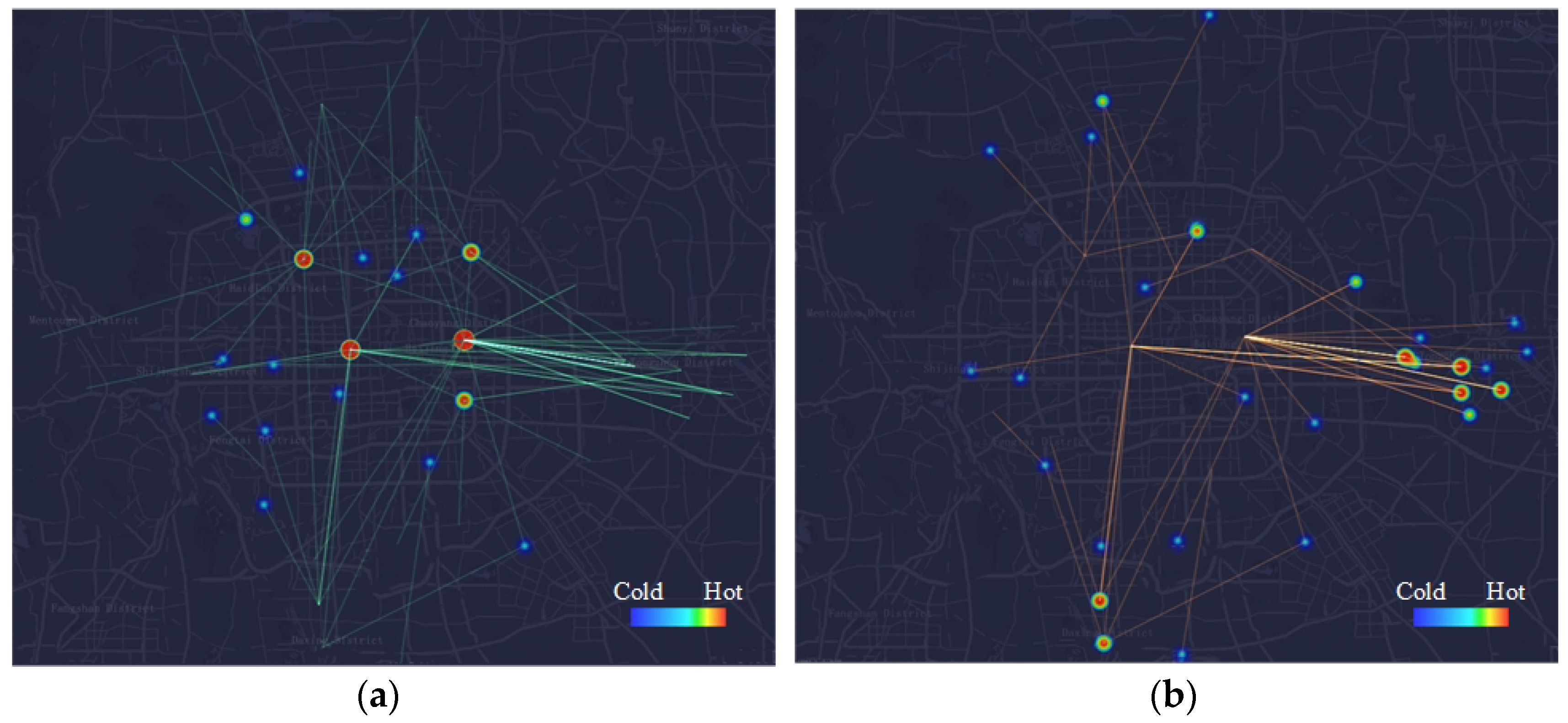
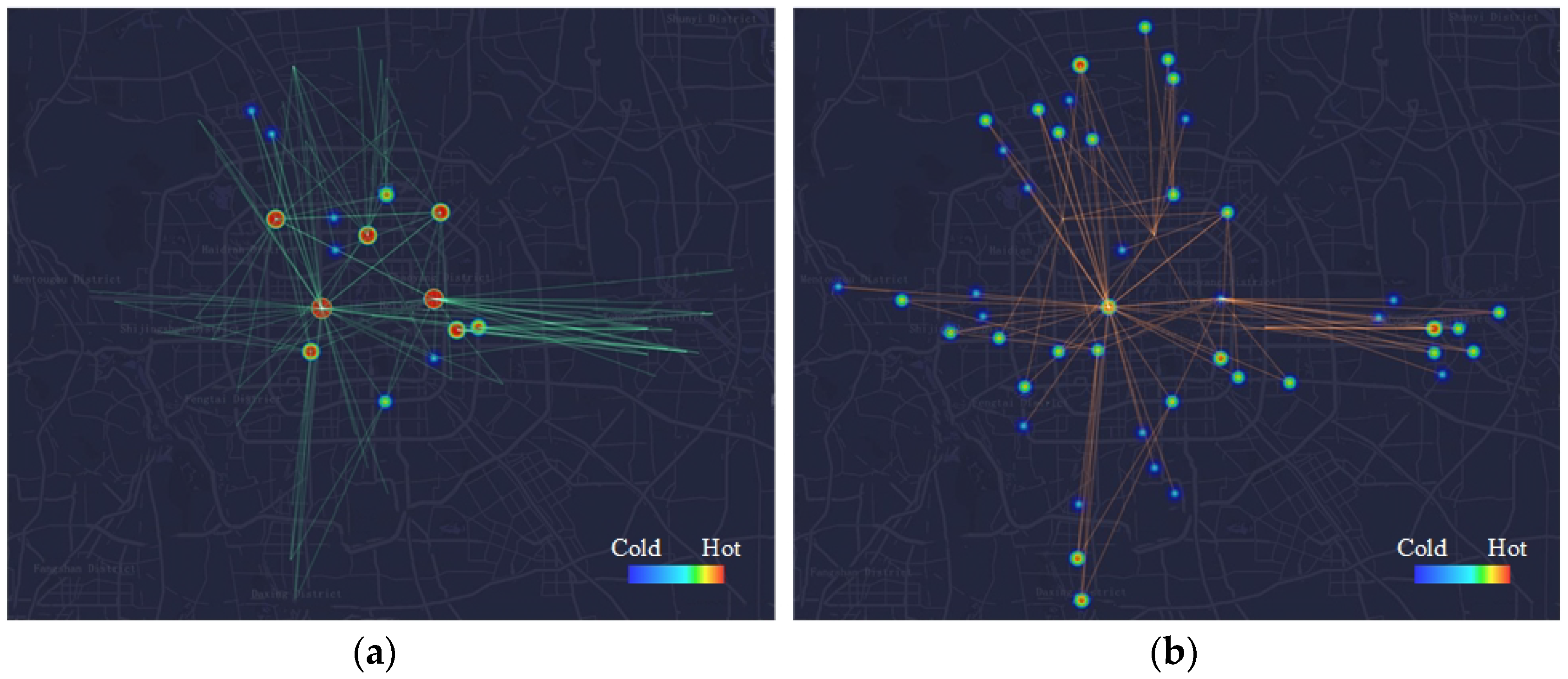
The current CB network of Beijing is distributed in urban and inner suburban areas, including Dongcheng, Xicheng, Haidian, Chaoyang, Fengtai, Shijingshan districts, and some large residential areas in inner suburbs such as Tiantongyuan, Huilongguan, Guanzhuang, and Huangcun. To evaluate the method proposed in this paper, potential CB routes extracted in these areas are brought out to compare with the current scheme, which contains routes recruiting passengers as well as routes having been operated by 29 March 2018. Figure 8 and Figure 9 show the CB routes of current scheme and potential scheme. In the figures, the green lines and yellow lines represent CB routes in morning peak hours and afternoon peak hours respectively. The thermodynamic circles are destination areas of the routes and the hotter the circle is, the more passengers it attracts. The comparative results of the number, total length, and average length of current and potential routes are presented specifically in Table 2. The coverage rate is represented by the proportion of the intersection of the current scheme and the potential scheme to the current scheme.
Compared with the current scheme, the total number of routes and the total length of operating routes extracted in potential scheme are greater. Thus, the potential scheme can serve more passengers and may have higher level of passenger service rate. In addition, the average length of potential scheme is slightly shorter than that of current scheme. The coverage rate reaches about 80 percent, demonstrating that the potential CB routes contains most of the current routes and the potential scheme generated by using the method of this paper is basically consistent with the current scheme.
It can be seen from Figure 8 and Figure 9 that in addition to Guomao, Jinrongjie, Zhongguancun, and Wangjing, Anzhen and Guanganmen also attract a large number of passengers in the morning peak hours. Meanwhile, the destination areas in the afternoon peak hours are relatively scattered. Routes from Guomao to Tongzhou, from Jinrongjie to Huilongguan, and Huangcun has the largest number of passengers. Note that both, the number of passengers to Jinrongjie in the afternoon peak hours, mainly from Guomao, is considerable. This is because Jinrongjie is an old prosperous living as well as shopping and business region. In general, the methodology proposed in this paper is feasible and effective for extracting CB routes.
4.3.2. Connections between Outer Suburban and Urban Areas
Another small group of clients CB serves is passengers who take round trips between outer suburban and urban areas. Because the distances of these routes are long, even some more than 50 km, travelling comfort becomes more important to passengers. The function of this class of CB service is somewhat similar to suburban lines of traditional buses with the advantages of providing door-to-door and one person one seat services. In this paper, 51 potential CB routes connecting outer suburban and urban areas are extracted using the method proposed in this paper, in which 28 are in the morning peak hours and 23 in the afternoon peak hours. As shown in Figure 10, the green arrow and the yellow arrow represent routes in morning peak hours and afternoon peak hours respectively. The arrow direction indicates travel direction.
It is easy to see the trip characteristics of these long distance travel passengers, basically travelling to urban areas in the morning and returning to outer suburban areas in the afternoon. Because people living in outer suburban, especially in large residential areas, need to take roundtrips for commuting in workdays, it is not hard to understand this phenomenon. Among the outer suburban areas, Yanjiao, Longquan, and Liangxiang towns are the three areas with the most passengers taking roundtrips between outer suburban and urban areas.
4.3.3. Routes in Outer Suburban Areas
According to this method, eight potential CB routes in Yanqing and Changping districts are extracted which meet the requirements of passenger number, regularity, and route length. But there is no known research showing whether the customized bus system is feasible in towns. Further investigation is needed to evidence the practicability of CB routes in towns.
5. Conclusions
The purpose of this study was to extract potential CB routes and then provide references for CB operators to conduct purposeful and effective investigation activities when planning CB network. A whole methodological framework, containing trip reconstruction, OD area division, and CB route extraction processes, was presented to achieve this goal based on bus smart card data. The proposed method introduced the idea of “from point to line” into the framework and concentrated on the “point” division and “line” clustering. In the OD area division process, a two-step division model was built in view of the uneven distribution of bus stops, which was characterized by the concept of “stop isolation” proposed in this paper. The DBSCAN algorithm was utilized twice to successfully divide the bus stops into different areas. In the CB route extraction process, identifying and clustering similar trips together was the core idea. The potential CB routes must satisfy three requirements: the number of passengers, regularity, and route length. An improved DBSCAN algorithm was used, in which the distance threshold extended from one spatial distance to three distance attributes related to spatial and temporal dimensions.
Taking Beijing as a case study, the results showed that the potential CB scheme planned using the proposed methodology had nearly 80% coincidence with the current CB scheme, thus proving the framework presented in this paper was feasible and reasonable. Besides, the potential CB scheme has more routes and longer total route distance than the current scheme. The result analysis of the case study provided references to the CB operator when planning CB network in Beijing. However it should be considered whether the parameter values are available for other cities when planning CB networks using the method introduced in this paper. Furthermore, as a personalized and exclusive service, the CB system needs to have the guarantee of passenger volume and market competitive advantages. In future research, the comparison with other public transport modes should be quantified to decide if a certain new CB route is necessary to open. Finally, only the areas and directions of potential CB routes are determined is this paper. If a certain route is planned to be operated, the specific boarding and alighting stops of the route must be confirmed.
Author Contributions
Data curation, J.L. and J.M.; Formal analysis, Q.O.; Investigation, J.L. and Q.O.; Methodology, J.L.; Supervision, Y.L.; Writing—original draft, J.L.; Writing—review & editing, Y.L. and J.M.
Funding
This research was funded by the National Key Technologies Research & Development Program under grant 2017YFC0804900.
Conflicts of Interest
The authors declare no conflict of interest.
References
- Ceder, A. Public Transit Planning and Operation: Theory, Modeling and Practice; Elsevier: Oxford, UK, 2007. [Google Scholar]
- Ceder, A. Public Transit Planning and Operation: Modeling, Practice and Behavior, 2nd ed.; CRC Press: Boca Raton, FL, USA, 2016. [Google Scholar]
- Liu, T.; Ceder, A.; Bologna, R.; Cabantous, B. Commuting by Customized Bus: A Comparative Analysis with Private Car and Conventional Public Transport in Two Cities. J. Public Transp. 2016, 19, 55–74. [Google Scholar] [CrossRef] [Green Version]
- Liu, T.; Ceder, A. Analysis of a new public transport service concept: Customized bus in China. Transp. Policy 2015, 39, 63–76. [Google Scholar] [CrossRef]
- Eiró, T.; Martínez, L.M.; Viegas, J.M. Configuration of Innovative Minibus Service in the Lisbon, Portugal, Municipality Spatial-Temporal Assessment. Transp. Res. Rec. 2011, 2217, 238–242. [Google Scholar] [CrossRef]
- Martínez, L.M.; Viegas, J.M.; Eiró, T. Formulating a New Express Minibus Service Design Problem as a Clustering Problem. Transp. Sci. 2015, 49, 85–98. [Google Scholar] [CrossRef]
- Guihaire, V.; Hao, J.K. Transit network design and scheduling: A global review. Transp. Res. Part A Policy Pract. 2008, 42, 1251–1273. [Google Scholar] [CrossRef] [Green Version]
- Chang, S.K.; Schonfeld, P.M. Optimization Models for Comparing Conventional and Subscription Bus Feeder Services. Transp. Sci. 1991, 25, 281–298. [Google Scholar] [CrossRef]
- Potts, J.F.; Marshall, M.A.; Crockett, E.C.; Washington, J. A Guide for Planning and Operating Flexible Public Transportation Services; TCRP Report; Rep. 140; Transportation Research Board: Washington, DC, USA, 2010. [Google Scholar]
- Vine, S.L.; Lee-Gosselin, M.; Sivakumar, A.; Polak, J. A new approach to predict the market and impacts of round-trip and point-to-point carsharing systems: Case study of London. Transp. Res. Part D Transp. Environ. 2014, 32, 218–229. [Google Scholar] [CrossRef]
- De Lorimier, A.; El-Geneidy, A.M. Understanding the Factors Affecting Vehicle Usage and Availability in Carsharing Networks: A Case Study of Communauto Carsharing System from Montréal, Canada. Int. J. Sustain. Transp. 2013, 7, 35–51. [Google Scholar] [CrossRef]
- Ma, J.H.; Yang, Y.; Guan, W.; Wang, F.; Liu, T.; Tu, W.Y.; Song, C.Y. Large Scale Demand Driven Design of a Customized Bus Network: A Methodological Framework and Beijing Case Study. J. Adv. Transp. 2017, 2017, 3865701. [Google Scholar] [CrossRef]
- Lyu, Y.; Chow, C.Y.; Lee, V.C.S.; Li, Y.H.; Zeng, J. T2CBS: Mining taxi trajectories for customized bus systems. In Proceedings of the IEEE INFOCOM WKSHPS, San Francisco, CA, USA, 10–14 April 2016; pp. 441–446. [Google Scholar]
- Pelletier, M.P.; Trépanier, M.; Morency, C. Smart card data use in public transit: A literature review. Transp. Res. Part C Emerg. Technol. 2011, 19, 557–568. [Google Scholar] [CrossRef]
- Chapleau, R.; Chu, K.K.A. Modeling Transit Travel Patterns from Location-Stamped Smart Card Data Using a Disaggregate Approach. In Proceedings of the 11th World Conference on Transport Research, Berkeley, CA, USA, 24–28 June 2007. [Google Scholar]
- Trépanier, M.; Tranchant, N.; Chapleau, R. Individual Trip Destination Estimation in a Transit Smart Card Automated Fare Collection System. J. Intell. Transp. Syst. 2007, 11, 1–14. [Google Scholar] [CrossRef]
- Munizaga, M.A.; Palma, C. Estimation of a disaggregate multimodal public transport Origin–Destination matrix from passive smartcard data from Santiago, Chile. Transp. Res. Part C Emerg. Technol. 2012, 24, 9–18. [Google Scholar] [CrossRef]
- Ester, M.; Kriegel, H.P.; Sander, J.; Xu, X. A density-based algorithm for discovering clusters in large spatial databases with noise. In KDD-96; AAAI Press: Portland, OR, USA, 1996; pp. 226–231. [Google Scholar]
- Beijing Transportation Smart Card Usage Survey; Beijing Transportation Research Center: Beijing, China, 2010.
- The 4th Comprehensive Transport Survey Summary Report; Beijing Transportation Research Center: Beijing, China, January 2012.
- Beijing Public Transport. Available online: http://dingzhi.bjbus.com/ (accessed on 29 March 2018).
Figure 1.
Flow chart of the framework.

Figure 2.
Process for retrieving the neighborhood of trip k.

Figure 3.
Daily temporal frequency distribution of transactions.

Figure 4.
Example of trip reconstruction.

Figure 5.
Examples of calculating 500 m-Stop Isolation. (a) Situation of stop A; (b) Situation of stop B.
Figure 5.
Examples of calculating 500 m-Stop Isolation. (a) Situation of stop A; (b) Situation of stop B.

Figure 6.
Sorted 500 m-Stop Isolation of stops (solid line) and the increase curve (dotted line).

Figure 7.
Result of OD area division (points in the same color means stops in one area).

Figure 8.
CB routes of the current scheme. (a) Morning peak hours; (b) Afternoon peak hours.

Figure 9.
CB routes of the potential scheme. (a) Morning peak hours; (b) Afternoon peak hours.

Figure 10.
Potential CB routes between outer suburban and urban areas.


Table 1.
Bus smart card data statistics.
| Date | Number of Trips | Number of Non-Noise Trips | Number of Trip Flows |
|---|---|---|---|
| 12 October | 3,061,963 | 1,498,210 | 2415 |
| 13 October | 3,445,015 | 1,678,388 | 2855 |
| 14 October | 3,409,252 | 1,656,289 | 2788 |
| 15 October | 3,381,776 | 1,637,186 | 2722 |
| 16 October | 2,867,636 | 1,362,541 | 2095 |
Table 2.
Beijing CB network contrast.
| Indicator | Current Scheme | Potential Scheme | Coverage Rate | |
|---|---|---|---|---|
| Morning Peak Hour | Number of Routes | 89 | 108 | 79.78% |
| Total Length (km) | 1378.045 | 1455.673 | 77.08% | |
| Average Length (km) | 15.484 | 13.478 | — | |
| Afternoon Peak Hour | Number of Routes | 60 | 82 | 85.00% |
| Total Length (km) | 916.723 | 1045.696 | 84.81% | |
| Average Length (km) | 15.279 | 12.752 | — | |
| Day Peak Hour | Number of Routes | 149 | 190 | 81.88% |
| Total Length (km) | 2294.768 | 2501.369 | 80.17% | |
| Average Length (km) | 15.401 | 13.165 | — | |
© 2018 by the authors. Licensee MDPI, Basel, Switzerland. This article is an open access article distributed under the terms and conditions of the Creative Commons Attribution (CC BY) license (http://creativecommons.org/licenses/by/4.0/).
Share and Cite
MDPI and ACS Style
Li, J.; Lv, Y.; Ma, J.; Ouyang, Q. Methodology for Extracting Potential Customized Bus Routes Based on Bus Smart Card Data. Energies 2018, 11, 2224. https://0-doi-org.brum.beds.ac.uk/10.3390/en11092224
AMA Style
Li J, Lv Y, Ma J, Ouyang Q. Methodology for Extracting Potential Customized Bus Routes Based on Bus Smart Card Data. Energies. 2018; 11(9):2224. https://0-doi-org.brum.beds.ac.uk/10.3390/en11092224
Chicago/Turabian StyleLi, Jing, Yongbo Lv, Jihui Ma, and Qi Ouyang. 2018. "Methodology for Extracting Potential Customized Bus Routes Based on Bus Smart Card Data" Energies 11, no. 9: 2224. https://0-doi-org.brum.beds.ac.uk/10.3390/en11092224
Note that from the first issue of 2016, this journal uses article numbers instead of page numbers. See further details here.