Complete Procedure for the Economic, Financial and Cost-Competitiveness of Photovoltaic Systems with Self-Consumption

Abstract

Nowadays, the integration of photovoltaic (PV) systems into the grid involves new and competitive ways to realize this. Thus, it is necessary to define procedures that not only include energy calculations but also incorporate economic and funding feasibility features. According to the literature review, there are numerous tools that are available to carry out a profitability analysis of a photovoltaic system. However, certain shortcomings have been identified, either in the definition of the economic and financial scenarios or in the results obtained, as they do not provide all the necessary information, do not use all the most common economic criteria, or in some cases the complexity and training requirements for their correct implementation may discourage their use. Therefore, in this paper a complete procedure that can be used as a preliminary decision tool prior to the design of an in-depth PV self-consumption system is proposed. Realistic input data makes it possible to not only obtain results for common economic and financial feasibility criteria (Net Present Value, Internal Rate of Return, Discounted Pay-Back Time and Net Cash Balance), but it also allow for a cost-competitiveness evaluation based on the Levelised Cost of Electricity (LCOE). The novel concept of the direct cost of PV self-consumed electricity is also introduced.

1. Introduction

In recent years, we have witnessed exponential growth in installed photovoltaic power around the world, and expectations are even more promising for the near future [1]. These figures position this technology as the leading driver not only of the renewable energy sector, but also as the main alternative for energy transitions [2,3].

This positioning has been possible mainly due to the strong drop in PV installation prices that this technology has experienced, where a decrease of around 80% has been detected in the last decade [4,5]. These figures, translated into unitary energy generation price, mean that currently, electricity produced from PV plants has become competitive with other energy sources [6,7,8,9]. Also, these significant changes in accumulated power have been possible because of the distributed generation characteristics of PV, which makes this technology accessible to standard homeowners under the recent self-consumption paradigm, and therefore convenient for small investors.

It is widely known that traditionally, PV systems have been differentiated as grid-connected and stand-alone. In the first case, the purpose is solely to inject energy into the grid and receive a proportional disbursement, while in the second case, the purpose is to provide electricity, with the help of a battery, to facilities isolated from the grid. Nowadays, this classification has become obsolete since photovoltaic technology has entered a new implementation paradigm, not based on location characteristics (isolated or not from the grid), but dependent on economic variables and generation-consumption profiles and their integration with the closest grid [10].

In this expansionist environment and new ways of integrating the PV technology into the grid, it is necessary to develop models that not only simulate the energy calculations, but that also incorporate tools for the evaluation of economic feasibility and for the funding analysis of the PV systems under these new approaches.

To evaluate the feasibility of a photovoltaic project, a technical, economic and financial analysis of the project must be carried out. For the economic evaluation, the classic criteria such as the Net Present Value (NPV), the Internal Rate of Return (IRR) or the Discounted Pay Back Time (DPBT) are normally used, whereas for the financial analysis, the Net Cash Balance criterion is applied.

A project may be feasible from the economic point of view and not from the financial perspective, i.e., the results obtained from the classic criteria may be positive, thus, encouraging investment from an economic perspective even though the cumulative annual cash balance may have some negative years, which means that from a finance point of view, there are several years of negative balance, which translates into potential bankruptcy of the project. This situation changes the parameters for financing a project, i.e., debt and equity need to be considered in order to achieve financial viability and acceptance of the project; otherwise, the project may be profitable but unaffordable [11].

There are already several studies in the scientific literature regarding the assessment of the economic feasibility of PV self-consumption systems, where the classic criteria are applied. In [12,13], an economic analysis of PV self-consumption systems is carried out using the Net Present Value criterion, whereas in [14] the profitability evaluation is done based on the Internal Rate of Return. In [15], photovoltaic systems in residential sectors without subsides are evaluated by assessing their profitability by means of the NPV and the DPBT. The NPV is once again the criterion selected for a techno-economic model focused on German households with PV systems plus battery storage from a domestic perspective [16]. In [17], small scale PV installations were analyzed in a representative selection of countries, including Australia, Brazil, China, Germany, Italy, Spain, United Kingdom, the United States of America, among others, in order to identify the systems with the best investment opportunities considering the new regulations for self-consumption. The methods used in [17] to evaluate economic feasibility are NPV, IRR, DPBP, and the Profitability Index (PI). These criteria were also applied in the economic assessment of self-consumption PV systems and large PV plants in [18,19,20], where the Levelised Cost of Electricity (LCOE) was also used.

Despite the large number of studies that include one of the aforementioned criteria, or a selection of them, it is not common for all of them to be applied at the same time in a single study. In addition, there is a lack of studies in the literature regarding the feasibility analysis of the funding of PV systems, assessed through the Net Cash Balance criterion, which may counteract or cancel the positive values of the economic criteria when the financial perspective of these projects is negative.

Many of the manuscripts found in the literature make use of dedicated PV simulation tools, which besides the energy assessment, incorporate features for the evaluation of the economic feasibility of a PV project, and sometimes, also their funding viability, e.g., RETScreen and PVSyst for which a license must be purchased. In [21], the techno-economic feasibility analysis of photovoltaic systems is carried out using the RETScreen tool for the evaluation of renewable energy technologies, which calculates a number of different criteria such as NPV, IRR, Simple Payback, Benefit-Cost Ratio (BCR) and the Energy Production Cost. In [22], the techno-economic feasibility of a 45kW grid-connected photovoltaic power plant in Iran is discussed using the professional tool PVSyst. In [23], a feasibility analysis of a 5 MW solar photovoltaic power plant for a higher educational institute campus in India to become self-sufficient in terms of energy requirements was undertaken, where the technical and financial viability of the proposed plant was done using PVSyst.

However, despite the appropriateness of using these commercial tools for the economic and financial assessment, they have some limitations in the methodology they use, such as not considering the tax issues (e.g., PVSyst), or not carrying out the feasibility analysis of the funding (Net Cash Balance) in the case of RETscreen. Neither of these tools provides the option for mixed funding simulation, i.e., equity capital (e.g., common stocks and preferred stocks) and debt (e.g., long-term loans, bonds and mortgage loans), that are normally used to fund capital investments.

There are also online financial tools that allow us to obtain an initial glimpse of the PV system’s feasibility, but the results obtained are very limited for making a proper decision on the feasibility of PV projects [24]. For example, the economic and financial parameters used as inputs are very scarce and they do not provide information regarding the Net Cash Balance criterion. Besides, they do not take percentages of self-consumption into account, so although these tools are simple, this is at the cost of losing essential preliminary information.

The objectives of this study were made in response to these weaknesses, and aims to properly address them.

In a methodical literature search, the authors found only one tool that provides a detailed economic feasibility and funding analysis. This is the NREL System Advisor Model (SAM) free distribution tool. In the reference mentioned above [23], the technical and financial viability of the proposed plant was also performed using SAM. However, as a drawback, the proper use of this tool requires extensive technical and economic knowledge on the part of the user, which makes it unattractive for someone who only needs a preliminary decision tool. Therefore, another objective of this study was to implement an economic and financial procedure in an easy-to-use tool.

Based on this context, the main purpose of this paper is to present a procedure which jointly evaluates the economic and funding feasibility of PV self-consumption systems, without the need for specialized tools, which require extensive prior technical and economic knowledge. This procedure also includes all the parameters to be taken into account in this type of analysis that are not considered in other existing tools, such as mixed funding, income tax, different types of self-consumption, distinct prices applicable to the electricity injected into the grid or self-consumed, tax depreciation or self-consumption index, among others. In order to develop and facilitate the use of the methodology proposed hereafter, the mathematical modelling of this procedure is supported by a MATLAB-based tool, which provides preliminary, quick results to future owners, investors, or entities interested in developing PV self-consumption systems.

As previously mentioned, the need to design a general procedure that can be used as a preliminary decision tool prior to the in-depth design of a photovoltaic system with self-consumption has been detected. Through the realistic definition of technical, economic and finance parameters, it will allow the user to not only obtain results related to the economic feasibility through the most widespread economic criteria (Net Present Value, Internal Rate of Return, Profitability Index, Discounted Pay- Back Time and Modified Profitability Index), but it will also allow the evaluation of its funding feasibility through the Net Cash Balance. In addition, this procedure will make it possible to assess the cost competitiveness of PV installations based on the Levelised Cost of Electricity. Moreover, if the type of self-consumption of the PV system being evaluated is direct, the tool as a novel concept, calculates the cost of direct self-consumption PV electricity (C_s) dependent on the self-consumption index (SCI).

Therefore, the main aim in this work is to propose a procedure for the evaluation of the economic and funding feasibility of PV self-consumption systems. First of all, the procedure of the economic and funding evaluation is described in detail in Section 2. This is followed by a brief description of the tool developed in Section 3. Subsequently, Section 4 shows the results of the application of this procedure to a general example in a realistic, random location, including a comparison with one of the commercial tools available in the market. In addition, a complete sensitivity analysis is included of the NPV, IRR, PI, LCOE and C_s, which is also required in the event of possible variations in most influencing parameters such as the global irradiation in the optimum inclined plane (H_OPT), SCI, nominal discount rate (d), unitary cost of a PV system (C_u), income tax rates (T), life cycle (N) or operation and maintenance costs. Finally, the most relevant conclusions are presented.

The procedure described in this paper overcomes the abovementioned drawbacks detected in the literature, showing a more complete methodology and including some novel concepts such as the cost of direct self-consumption PV electricity (Cs). The tool that implements the mathematical procedure is important because although it is somewhat complex, the solution is transparent to the end user and it offers, as a result, information that is useful and relevant to the design of the system.

2. Methodology

The developed tool provides information regarding the economic and funding feasibility of a PV self-consumption project. All the complex mathematical procedures described below has been implemented in the tool, completely transparent to the end-user, so they do not need to have advanced knowledge in these concepts.

In this paper, the economic feasibility analysis is based on the Net Present Value, Internal Rate of Return, Profitability Index, Modified Profitability Index and Discounted Pay-Back Time. Criteria such as NPV, IRR, PI and PIM address the profitability, while DPBT aims to measure investment liquidity. The funding feasibility analysis is conducted by means of the Net Cash Balance. The model used to estimate the cost of generating electricity from the photovoltaic system is based on the Levelised Cost of Electricity. The economic feasibility models have already been introduced in previous works [25,26,27], however, this innovative model incorporates the option of self-consumption under different types, in addition to the calculation of the cost of direct PV self-consumed electricity, and the feasibility analysis of the financing by means of the Net Cash Balance concept.

2.1. Net Present Value

The Net Present Value of a project is defined as the difference between the present values of the cash inflows (CI, in €) and cash outflows (CO, in €) generated by the investment over the lifetime of the project (N) [25,28]. Mathematically, it can be written as follows:

$$\mathrm{NPV}=PW\left[CI\left(N\right)\right]-PW\left[CO\left(N\right)\right]$$

(1)

PW[CI(N)](€) is the present worth (value) of the cash inflows over the lifetime of the project. Regarding this parameter, cash inflows are partly obtained by means of the annual PV electricity generated that is used for self-consumption (E_PVs, in kWh) and consequently saved, instead of buying it from the grid at a given price (p_s, in €/kWh). Additionally, cash inflows are obtained by the annual electricity generation (E_PVg, in kWh), partly fed into the grid, which may be compensated at a different price (p_g, in €/kWh). Bearing in mind all these considerations, the present worth of the cash inflows from a PV system PW[CI(N)] may be written as:

$$PW\left[CI\left(N\right)\right]=p_s{E}_{PVs}\left(1-T\right)\frac{K_s\left(1-K_s^N\right)}{1-K_s}+p_g{E}_{PVg}\left(1-T\right)\frac{K_g\left(1-K_g^N\right)}{1-K_g}$$

(2)

where the factors K_s and K_g are just a parameter used to simplify the previous equation and they are obtained from the following expressions: K_s = (1 + rp_s)·(1 − r_d)/(1 + d) and K_g = (1 + rp_g)·(1 − r_d)/(1 + d) [29,30].

rp_s (%) and rp_g (%) stand for the annual escalation rate of the electricity price that is self-consumed and injected into it, respectively, while factor r_d (%) is the annual degradation rate of the efficiency of the PV modules. The variable T is the tax income rate (%) applicable to the income whereas d is referred to as the nominal discount rate (%).

As noted above, Equation (2) is defined for the most general case. However, if the annual electricity generated by the photovoltaic system is completely used for self-consumption, this equation can be simplified by eliminating the second term:

$$PW\left[CI\left(N\right)\right]=p_s{E}_{PVs}\left(1-T\right)\frac{K_s\left(1-K_s^N\right)}{1-K_s}$$

(3)

Likewise, if the annual PV generated electricity is entirely sold to the grid, Equation (2) is simplified:

$$PW[CI\left(N\right)]=p_g{E}_{PVg}\left(1-T\right)\frac{K_g\left(1-K_g^N\right)}{1-K_g}$$

(4)

The second term of the NPV equation stands for the present worth of the cash outflows from the PV system PW[CO(N)] (€) and it is calculated by adding the initial investment cost of the PV system (PV_I) plus the present worth of its operation and maintenance cost (PW[PV_OM(N)]) and subtracting the present worth of the tax depreciation PW[DEP(N_d)] during the system life cycle (N):

$$PW\left[CO\left(N\right)\right]=P{V}_I+PW\left[P{V}_{OM}\left(N\right)\right]-PW\left[DEP\left(N_d\right)\right]T$$

(5)

where the initial investment (PV_I) is calculated by the unitary cost of the PV system times the installed nominal power PV_I = C_u·P.

When analyzing the cash outflow equation, the present worth of the operation and maintenance cost during the life cycle of the system can be expressed as:

$$PW\left[P{V}_{OM}\left(N\right)\right]=P{V}_{OM}\left(1-T\right)\frac{K_p\left(1-K_p^N\right)}{1-K_p}$$

(6)

In the previous equation, (PV_OM, €) stands for the annual operation and maintenance expenditure which is assumed to be constant over the life cycle of the system, with the exception of an annual escalation rate (r_OM, in %) included in the factor K_P = (1 + r_OM)/(1 + d).

Finally, in those scenarios where there is a deductible tax depreciation, its impact is considered through the following expression of its present worth of tax depreciation PW[DEP(N_d)].

$$PW\left[DEP\left(N_d\right)\right]={\displaystyle \sum }_{n=1}^{N_d}\frac{DE{P}_n}{{\left(1+d\right)}^n}$$

(7)

In this equation, DEP_n (€) represents the tax depreciation corresponding to year n and N_d is the period of time over which an investment is amortized for tax purposes. Although the method used in the tax depreciation may differ from country to country, readers should refer to national tax laws. For example, if the tax depreciation is assumed to be linear and constant over a given period of time, the present worth of the tax depreciation can be estimated using the following equation:

$$PW\left[DEP\left(N_d\right)\right]=DE{P}_y\frac{q\left(1-q^{N_d}\right)}{\left(1-q\right)}$$

(8)

where DEP_y (€) is the fixed annual tax depreciation for the PV system and q = 1/(1 + d).

One criteria that indicates the project’s feasibility is when the calculated NPV is positive after using a sustainable discount rate. On the other hand, a negative NPV indicates that the project should not be considered.

2.2. Internal Rate of Return

The Internal Rate of Return (IRR) of an investment project is the value of the discount rate d that leads to NPV = 0. Furthermore, the IRR for a given project can be defined as the real interest rate of the initial investment that the project is lent during its useful life to achieve the same profitability [31]. Therefore, IRR is the value of d that satisfies:

$$0=PW\left[CI\left(N\right)\right]-PW\left[CO\left(N\right)\right]$$

(9)

This equation leads to the calculation of a “gross” Internal Rate of Return. However, since most projects use financial mechanisms, the net Internal Rate of Return (IRR_n) provides a more realistic assessment. In order to obtain IRR_n, the Weighted Average Cost of Capital (WACC), i.e., the cost of financing to the investor, is subtracted from the gross IRR as shown in equation 10:

$$\mathrm{IRRn}=\mathrm{IRR}-\mathrm{WACC}$$

(10)

Under this criterion, a project should be accepted when the IRR is greater than the company’s cost of capital and the project with an IRR lower than the WACC must be rejected, otherwise, the cost of financing will be greater than the return on investment. Therefore, the expected return must be greater than that required for a project to be economically feasible [27,32].

2.3. Discounted Pay-Back Time

The Discounted Pay-Back Time (DPBT, in years) is the number of years required for the sum of the cash flows generated by the project to cover the initial investment cost and it is an indicator of liquidity and risk. It is calculated with the formulae:

$$P{V}_I=PW\left[CI\left(DPBT\right)\right]-PW\left[CO\left(DPBT\right)\right]$$

(11)

$$P{V}_I=PW\left[CI\left(DPBT\right)\right]-PW\left[P{V}_{OM}\left(DPBT\right)\right]+PW\left[DEP\left(N_d\right)\right]T$$

(12)

where PW[CI(DPBT)] (€) is the present worth of the cash inflows generated over DPBT and PW[PV_OM(DPBT)] (€) is the present worth of the operation and maintenance cost over DPBT.

If N_d is greater than DPBT, the depreciation term in the previous equation should be rewritten as follows:

$$P{V}_I=PW\left[CI\left(DPBT\right)\right]-PW\left[P{V}_{OM}\left(DPBT\right)\right]+PW\left[DEP\left(DPBT\right)\right]T$$

(13)

where PW[DEP(DPBT)] (€) is the present worth of the tax depreciation over DPBT.

The acceptability of the investment is determined by the payback period required by the investor. Therefore, the investment should be accepted when the DPBT is less than the return on investment period required by the investor, otherwise the project must be rejected.

2.4. Profitability Index and Modified Profitability Index

The Profitability Index (PI) of an investment project is defined as the ratio between the present worth of the cash inflow and the present worth of the operation and maintenance cost during the lifetime of the PV system plus the present worth of the tax depreciation PW[DEP(N_d)], over the initial investment cost (PV_I).

$$\mathrm{PI}=\frac{PW\left[CI\left(N\right)\right]-PW\left[P{V}_{OM}\left(N\right)\right]+PW\left[DEP\left(N_d\right)\right]·T}{P{V}_I}$$

(14)

The use of this criterion to assess the profitability implies that the project is feasible when PI is greater than one, so if several projects are to be evaluated, the one with the highest PI should be preferable.

The Modified Profitability Index of an investment project is defined as the ratio between the Net Present Value and the initial investment cost (PV_I).

$$\mathrm{PIM}=\frac{\mathrm{NPV}}{P{V}_I}$$

(15)

If this criterion is used, the project is profitable when PIM is positive, while negative values of this parameter represent unprofitable investments.

2.5. Levelised Cost of Electricity

The Levelised Cost of Electricity is defined as the constant and theoretical cost of PV electricity production over its entire lifecycle, expressed in €/kWh. Additionally, LCOE enables the comparison of costs of the electricity generated by different technologies. Consequently, the use of LCOE is increasingly adopted as a metric by many solar stakeholders. The Levelised Cost of Electricity of a PV system can be expressed as:

$$\mathrm{LCOE}=\frac{PW\left[CO\left(N\right)\right]}{E_{PV}·{\sum }_{n=1}^N\frac{{\left(1-r_d\right)}^n}{{\left(1+d\right)}^n}}$$

(16)

2.6. Cost of Direct PV Self-Consumed Electricity

In a PV self-consumption system, C_S is defined as the unitary cost of direct PV self-consumed electricity over its entire lifetime, expressed in €/kWh. We refer to direct PV self-consumption, where there is no remuneration for surplus electricity. The estimation of Cs can be calculated as:

$${\mathrm{C}}_{\mathrm{S}}=\frac{\mathrm{LCOE}\cdot E_{PV}\cdot {\sum }_{n=1}^N\frac{{\left(1-r_d\right)}^n}{{\left(1+d\right)}^n}}{E_{PVs}\cdot {\sum }_{n=1}^N\frac{1}{{\left(1+d\right)}^n}}$$

(17)

E_PV (kWh/year) is the annual PV electricity generated and E_PVs (kWh/year) corresponds to the annual PV electricity that is directly self-consumed.

2.7. Weighted Average Cost of Capital

The calculation of the WACC is done following the procedure introduced in previous works [25,32]. The project investment is usually financed by means of debt or equity capital. In the case where the initial investment PV_I is financed through a loan (PV_l)—debt—and the remainder by means of the issue of stocks (PV_s)—equity capital—then PV_IN = PV_l + PV_s.

In order to consider all possible scenarios, a subsidy for the initial investment cost (PV_IS) is also included for the cases where a certain energy policy includes these sorts of supporting mechanisms. In those cases where a subsidy in the form of grants or rebates, among others, is applicable, the amount to be financed through a loan and issue of stocks would be: PV_I − PV_IS = PV_l + PV_s. Hence, the initial investment cost may be expressed as:

$$\begin{array}{l}P{V}_I=\left(P{V}_l\frac{i_l\left(1-T\right)}{1-{\left(1+i_l\left(1-T\right)\right)}^{-N_l}}\frac{q\left(1-q^{N_l}\right)}{1-q}\right)+\\ \left(d_{s}P{V}_s\frac{q\left(1-q^N\right)}{1-q}+P{V}_s{p}^N\right)+\left(\frac{P{V}_{IS}}{N_{IS}}T\frac{q\left(1-q^{N_{IS}}\right)}{1-q}\right)\end{array}$$

(18)

The first term in brackets of Equation (18) is related to the loan (PV_l), i.e., the amount of the initial investment that is borrowed at an annual interest (i_l) to be repaid in N_l years. A possible tax rate (T) influence is also included.

The second term of the equation 18 corresponds to the equity share (PV_s), with an annual retribution in the form of dividends (d_s) as a return on equity. This amount must be paid in full at the end of the project life cycle (N years).

The last term of the previous equation represents the investment subsidy (PV_IS) in those scenarios where it is applicable. It should be noted that PV_IS is also taxable for a specific period of time during which the investment subsidy is amortized (N_IS, years) and that the amount of the subsidized investment is non-repayable.

The left-hand side of Equation (18) only equals its right-hand side if the selected value of d is equal to the WACC of the investment, that is, how much the chosen financing costs.

2.8. Net Cash Balance

The Net Cash Balance is performed annually and is obtained from the difference between cash inflows and outflows related to the project. The investment will be feasible from the financial point of view provided that all annual accumulated Net Cash Balances are positive. Net Cash Balance can be written as:

$$\begin{array}{l}T{S}_n=\left(p_s{E}_{PVs}{\left(1+\Delta p_s\right)}^n+p_g{E}_{PVg}{\left(1+\Delta p_g\right)}^n\right)·\left(\left(1-T\right){\left(1-r_d\right)}^n\right)-\\ -\left(P{V}_{OM}\left(1-T\right){\left(1+r_{O\&M}\right)}^n\right)+DE{P}_{y}T·a_1-\\ -P{V}_l·\frac{i_l\left(1-T\right)}{1-{\left(1+i_l\left(1-T\right)\right)}^{-N_l}}·a_2-d_s·P{V}_s-P{V}_s·a_3-\frac{P{V}_{IS}}{N_{IS}}T·a_4\end{array}$$

(19)

where a₁ = 1 if n ≤ N_d or a₁ = 0 if n >N_d; a₂ = 1 if n ≤ N_l or a₂ = 0 if n > N_l; a₃ = 1 if n = N or a₃ = 0 if n ≠ N and a₄ = 1 if n ≤ N_IS or a₄ = 0 if n > N_IS.

3. Description of the Tool Developed to Facilitate the Procedure

The techno-economic analysis of a PV system is a tool, based on MATLAB®, developed by the IDEA Solar Research group of the University of Jaen, with the purpose of facilitating the economic and funding feasibility assessment of a PV project. It also includes the estimation of costs of the electricity generated, based on the Levelised Cost of Electricity, which it is useful for determining its competitiveness. A remarkable feature is the inclusion of self-consumption in this analysis.

This tool will help the user to visualise not only the most common feasibility economic criteria of a project such as the Net Present Value, Internal Rate of Return, Profitability Index, Modified Profitability Index and the Discounted Pay-Back Time, as described in the methodology, but it will also provide information regarding its funding feasibility in terms of the Net Cash Balance. Additionally, the Weight Average Cost of Capital is calculated and can be used as a nominal discount rate.

In the direct self-consumption analysis, where surplus energy is not remunerated, the cost of direct PV self-consumed electricity (C_S) is estimated and also the self-sufficiency index (SSI), which indicates the percentage of electricity consumed at home that it is provided by the PV system

In order to expand and complement the information offered, a graphical sensitivity analysis section is included. In this feature, the impact that certain input variables may have on IRR, NPV, PI, LCOE and C_s is provided. The variations in global irradiation on the optimal inclined plane (H_OPT), SCI, nominal discount rate (d), unitary cost of a PV system (C_u), income tax rates (T), life cycle (N) and annual operation and maintenance cost (C_O&M) are the most influential inputs chosen, and which may be the most critical for the economic assessment of a PV system.

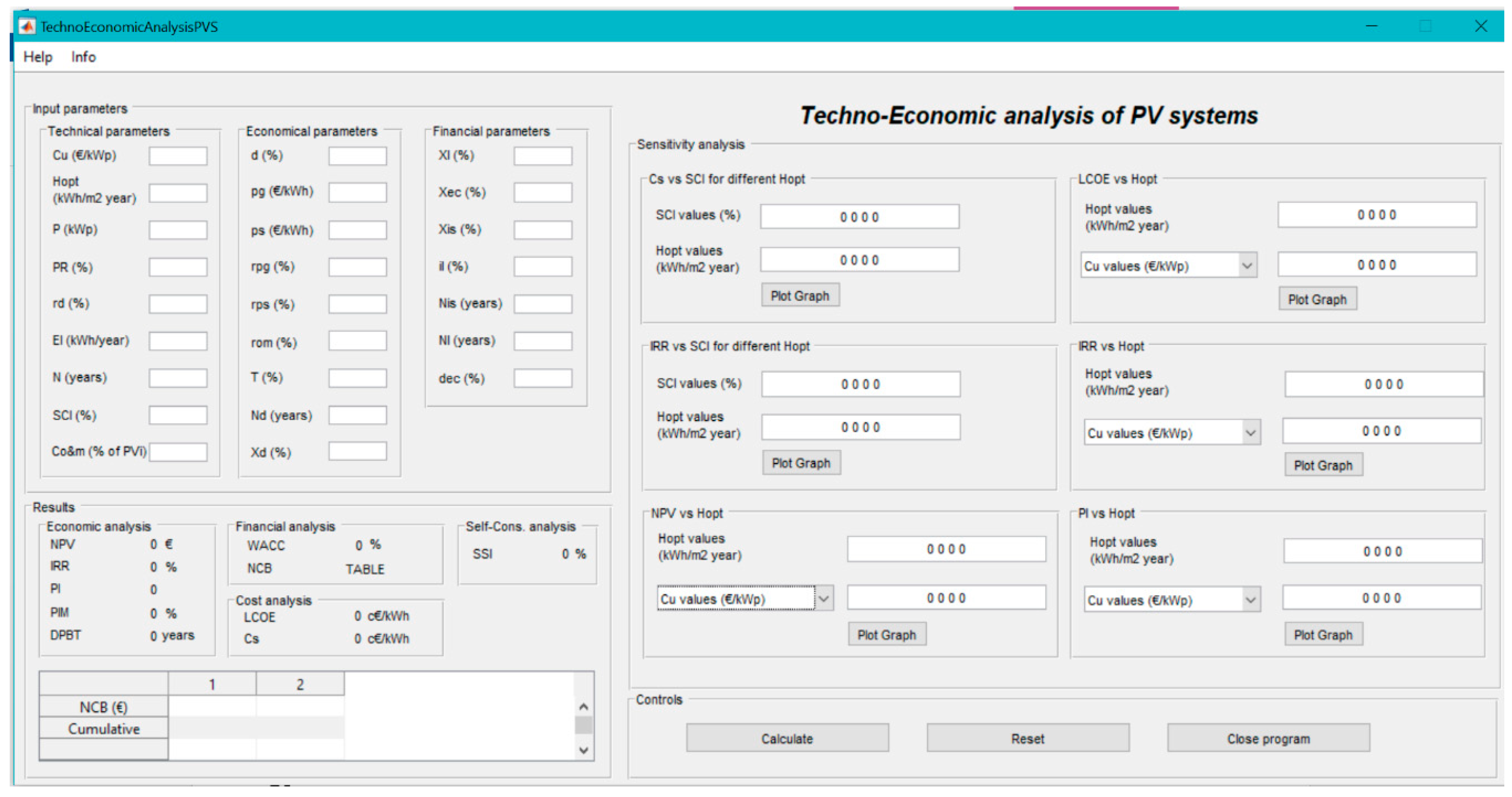
The main home screen of the tool is shown in Figure 1, where the 3 main aspects of this tool are shown, i.e., input parameters, results and sensitivity analysis.

The Result section of the main screen shows not only the resulting data from the economic, cost and self-consumption calculations, but it also provides a table which shows the NCB during the entire lifetime of the installation, which enables the user to identify possible lack of liquidity scenarios and make decisions based not only on economic feasibility, but also on the feasibility of the funding of the PV systems.

The Sensitivity section offers the users a visual comparison of the effect that the variation in certain parameters may have on the results. There are 6 different analyses available in the tool: (1) C_S as a function of the SCI for variations of H_OPT;( 2) LCOE as a function of H_OPT for variations of: C_u, d, C_O&M, N or T; (3) IRR as a function of SCI for variations of H_OPT; (4) IRR as a function of H_OPT for variations of: C_u, d, C_O&M, N or T; (5) NPV as a function of H_OPT for variations of: C_u, d, C_O&M, N or T and (6) PI as a function of H_OPT for variations of: C_u, d, C_O&M, N or T.

In order to plot the graphs, two vectors of the aforementioned data must be entered. Once the graph is created, users can zoom it, write on it, save it and select the different plotted points so that they can fully understand the results of the analysis.

This tool is freely offered by the University of Jaén to any professionals in the sector, investors or prospective PV system owners who are interested in it (https://drive.google.com/drive/folders/130LzYTP5xXXFGvf70Zisf1cbI8s27WiK?usp=sharing). In case there is any problem with the link, any interested user can also contact the corresponding author by e-mail to obtain the most updated version of the tool.

4. Results

An example of application is included in this paper to assess the validity of the proposed methodology. A residential photovoltaic system located in Madrid (Spain) was chosen, although any other location in the world for which the necessary data are available for simulation could have been also selected. In this example, a direct PV self-consumption system in which excess energy is injected into the grid without any remuneration has been chosen.

The input parameters needed to perform the procedure for this example (see

Table 1. Parameters defined for the study case in Madrid (Spain).

INPUT PARAMETERS
Factor	Values	Units
Technical Parameters
Cu	1250	€/kWp
HOPT	2040	kWh/(kWp·yr)
P	3.5	kWp
PR	75	%
rd	0.5	%/yr
EL	5580	kWh/yr
N	25	yr
SCI	60	%
CO&M	1.5	% of PVI
Economical Parameters
d	6.02	%
pg	0	€/kWh
ps	0.1575	€/kWh
rOM	1.45	%
rpg	0	%
rps	1.45	%
T	0	%
Nd	0	yr
Xd	0	%
g	1.45	%
Financial Parameters
Xl	70	%
Xec	30	%
XIS	0	%
il	5	%
NIS	0	yr
Nl	20	yr
dec	6	%

) includes all the necessary data for the calculation methodology described in Section 2. These parameters are divided into technical, economic and financial factors. The meaning of each parameter is listed in the Annex of this paper.

The technical parameters can be easily obtained once the user has defined the size (power, P) and location of the PV system, and they depend on the assumptions made and the characteristics of the system.

The energy generated by the PV installation will depend on the received solar radiation available in the selected location. The global irradiation on the optimal inclined plane (H_OPT, in kWh/(m² year)) is an input that the user must enter according to the characteristics of the place. An available tool to estimate this parameter in a wide selection of locations could be through the online PVGIS [33], which has the meteorological and simulation tools for these calculations.

Another parameter related to the energy term is the Performance Ratio (PR), which corresponds to the sources of energy losses. Normally, according to the existing literature, its value is in the range from 0.70 to 0.80 [34,35,36,37,38]. Besides these losses, the intrinsic degradation of the modules during their lifetime have to be considered. Normally, an annual degradation rate (r_d) of 0.5% is assumed [39,40] during the 25 years of the duration of the system (N).

Another technical parameter to be considered is the initial investment cost of the system, which is very variable and dependent on the country where the PV installation is located [5,41]. The unitary investment cost (C_u) used in this procedure represents the cost per kWp of a photovoltaic system. One of the last reports available consider this as 1053 US$/kW to 3550 $/kW for residential PV, whereas in the case of commercial or industrial PV installations, the unitary prices range from 1050 $/kW to 2030 $/kW [41].

The definition of an annual price for operation and maintenance tasks is normally recommended to be between an annual 0.5% and 1.5% of the investment cost for small PV installations [42]. Additionally, these costs will also be influenced by an annual escalation rate (r_OM). This input economic parameter is set equal to the value of the annual inflation defined by the country analysed.

The last input technical parameters are the annual total household electricity consumption E_L and the SCI the owner requires. These data need to be provided by the end-user at the location where the PV will be installed.

The economical parameters are the other input dataset that is entered into the tool. Income tax rates are applicable only for PV systems in the commercial and industrial segment, and this depends on the country´s regulation. For the study case of Madrid (Spain), a value of T = 0% has been set as it is a residential PV system [43]. The depreciation for tax purposes is assumed to be linear and constant over a given period of time (N_d).

In addition, the price at which the surplus electricity is sold to the grid (p_g) and the price of the self-consumed electricity (p_s), which it is normally equal to the retail electrical tariff, is inserted, provided that the photovoltaic project under analysis is for self-consumption. It is necessary to define an annual escalation rate of the electricity price that is self-consumed (r_ps) and fed into the grid (r_pg), as they do not remain constant. Normally, they are linked to the evolution of electricity markets, which is difficult to forecast and in case of lack of information, is set equal to the value of the annual inflation defined for each country.

The financial parameters considered in the developed procedure reflect different types of financing by means of loans, equity capital and subsidies, as detailed in Section 2, therefore, it offers the user a range of funding possibilities that facilitate their decision making. In this study case, following the trend of similar studies found in the literature, the percentage of the initial investment financed with debt (X_l) is set as 70%, whereas the equity capital share (X_ec) is set as the remaining 30% [44]. This data can be extrapolated to neighbouring countries with a similar economic context, but in the case of not-so stable economies, the share of equity and debt in the project is recommended to be 50% [45].

The loan interest and dividend percentage will depend on the financial product offered by the bank, as well as on the return required by the investor for the equity share.

This use of a variety of input parameters is the strong and differentiating characteristic of the procedure compared to the existing state-of-the-art methods reviewed in Section 1, as it offers a wide range of possibilities to the users, who can simulate thousands of combinations under different assumption scenarios

A summary of all the values assumed for every parameter that defines the case study are gathered in Table 1.

The economic, financial and cost results of this example (see

Table 2. Results obtained for the study case in Madrid (Spain).

RESULTS
Economic Analysis Results		Financial Analysis Results
NPV	1763.3 €	WACC	6.02%
IRR	9.8%	NCB	(see Table 3)
PI	1.4	Cost Analysis Results
PIM	40%	LCOE	8.23 c€/kWh
DPBT	14.22 years	Cs	13.71 c€/kWh

) show the viability of this PV project. The PV system is economically feasible because the NPV is positive and the IRR is higher than the WACC. In addition, the system is competitive in cost because C_S is lower than the price of electricity from the grid, which leads us to conclude that grid parity has been achieved. However, the aim of this example is not to show the economic feasibility of this case, but to reinforce the idea of the ease of use of the procedure, materialised in the proposed tool, and the speed with which results can be obtained to give an initial idea of the economic viability of a PV project.

Besides the aforementioned results and as stated previously, the Net Cash Balance (NCB) offers information regarding the funding feasibility of the PV system. In this example, the data obtained for each year of the 25 of the life-time of the system, are reproduced in

Table 3. Net Cash Balance Result of the example.

NET CASH BALANCE RESULTS
Year	NCB (€)	Cumulative (€)
1	100.06	100.06
2	103.91	203.97
3	107.79	311.76
4	111.71	423.47
5	115.65	539.12
6	119.63	658.75
7	123.64	782.39
8	127.68	910.07
9	131.76	1041.83
10	135.86	1177.69
11	140.01	1317.7
12	144.18	1461.88
13	148.39	1610.27
14	152.63	1762.9
15	156.91	1919.81
16	161.22	2081.03
17	165.56	2246.59
18	169.94	2416.53
19	174.36	2590.89
20	178.81	2769.7
21	429.04	3198.74
22	433.56	3632.3
23	438.12	4070.42
24	442.72	4513.14
25	−865.15	3647.99

. It can be observed that the cumulative NCB is positive during the lifetime of the system, therefore, the investment is also financially feasible. The negative value of the last term corresponds with the date of the return of the capital that was invested as equity, as it was previously mentioned in Section 2.7.

Concerning the sensitivity analysis, in this example a selection of 5 studies was carried out depending on the variable combinations. The first step is the introduction of two vectors with the steps of variations of the parameters involved. They are used to solve the equation shown in the methodology by combining the solutions into a single graph.

Table 4. Sensitivity analysis for combination of variables.

Cs vs SCI for different Hopt		LCOE vs Hopt for different Cu
SCI values (%)	(20 40 60 80 100)	Hopt values (kWh/m2 year)	(1200 1500 1800 2100 2400)
Hopt values (kWh/m2 year)	(1200 1500 1800 2100 2400)	Cu values (€/kWp)	(500 800 1100 1400 1700)
IRR vs SCI for different Hopt		IRR vs Hopt for different Cu
SCI values (%)	(20 40 60 80 100)	Hopt values (kWh/m2 year)	(1200 1500 1800 2100 2400)
Hopt values (kWh/m2 year)	(1200 1500 1800 2100 2400)	Cu values (€/kWp)	(500 800 1100 1400 1700)
NPV vs Hopt for different Cu
Hopt values (kWh/m2 year)	(1200 1500 1800 2100 2400)
Cu values (€/kWp)	(500 800 1100 1400 1700)

shows the range of variations and the variable combinations.

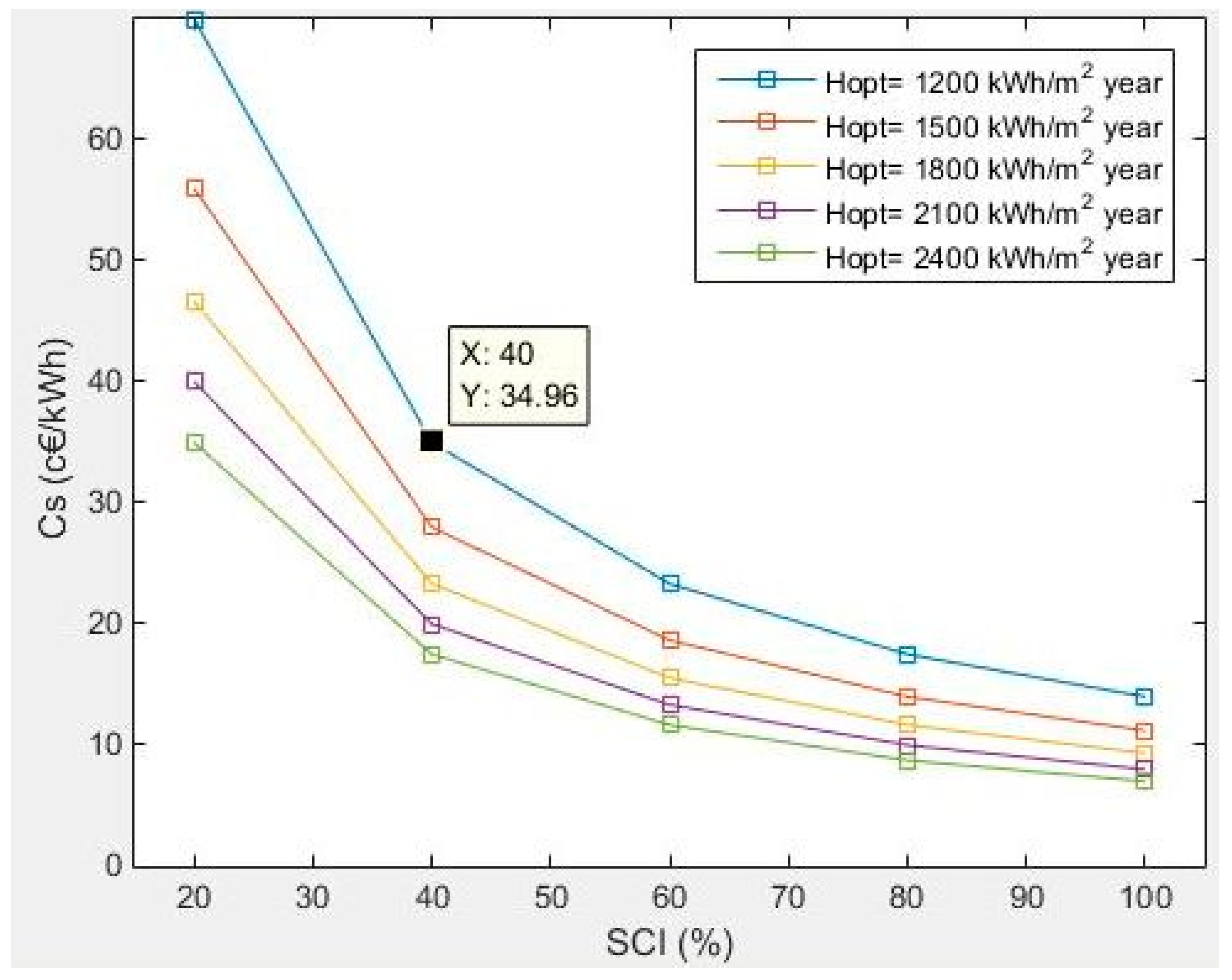
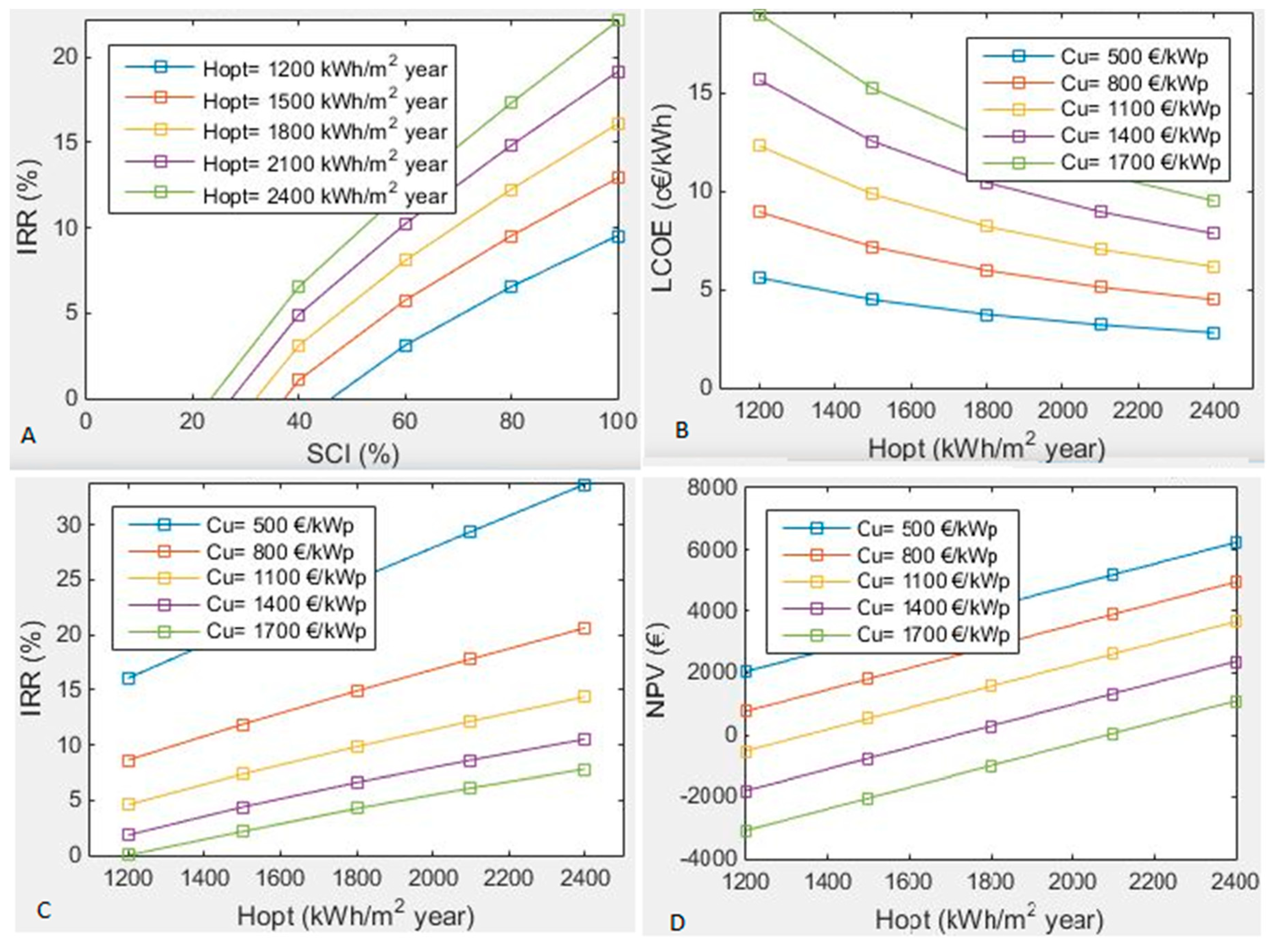
If Figure 2 is analysed, different C_S values can be obtained depending on the self-consumption index scenario considered in the PV system (variations from 20% to 100% in this case). The same figure also enables the possibility of simulating the behaviour of the PV system for different annual global irradiations at the optimal tilt angle (H_OPT) ranging from 1200 to 2400 kWh/(m² year). The rest of the sensitivity analysis result plots are shown in Figure 3.

Considering an average electricity price (p_s) of 16 c€/kWh for the residential sector in Spain, for consumption ranging from 5000 kWh to 15,000 kWh, and assuming the best self-consumption scenario possible, i.e., SCI = 100%, in any case of the H_OPT scenarios from Figure 2, the estimated value of C_S is equal to LCOE. Furthermore, under the input characteristics of this example, whose results are also shown in Figure 2, C_S values are lower than the electricity price for residential consumers for some values SCI and H_OPT, except for irradiation levels below 1200 kWh/(m² year). Therefore, in the scenario considered and under the established premises, a residential PV self-consumption system is competitive, thus reaching parity with the grid.

The sensitivity analysis also enables us to identify scenarios in which a residential PV system is not competitive, i.e. when the C_S value is higher than the electricity price for residential consumers. It can be observed that this undesirable situation is reached when the SCI is lower than 50%, 56%, 63% and 80% for H_OPT values of 2400, 2100, 1800 and 1500 kWh/(m² year) respectively.

5. Discussion

Besides the explanation of the features of the procedure proposed and the tool that has been developed, we also compared it with other commercial tools and with the results from any available research manuscripts.

The professional tools for the design of PV systems that are fee-based have certain limitations, as described in the Introduction, apart from the fact that the licenses are very expensive and may not be worthwhile for an unprofessional user who only needs an easy-to-use tool that allows a prior assessment of the feasibility of a photovoltaic system. Therefore, it is more interesting to make this comparison with an open source tool. For this purpose, a feasibility analysis of a self-consumption photovoltaic system was carried out with the System Advisor Model (SAM) tool, developed by NREL, whose results will be compared with the outputs from the application of the procedure described in this work.

A different example from the previous section is proposed with the aim of reinforcing the validity of the tool developed by analyzing a different location with different input parameters. The data of the system input parameters are shown in

Table 5. Parameters defined for the comparison between the procedure and commercial tools.

INPUT PARAMETERS
Factor	Values	Units
Technical Parameters
Cu	2860	$/kWp
HOPT	2095	kWh/(kWp·yr)
P	4	kWp
PR	75	%
rd	0.5	%/yr
EL	6019	kWh/yr
N	25	yr
SCI	100	%
CO&M	0.7	% of PVI
Economical Parameters
d	5.4	%
pg	0	$/kWh
ps	0.16	$/kWh
rOM	2.5	%
rpg	0	%
rps	2.5	%
T	0	%
Nd	0	yr
Xd	0	%
g	2.5	%
Financial Parameters
Xl	70	%
Xec	30	%
XIS	0	%
il	5	%
NIS	0	yr
Nl	20	yr
dec	6	%

(they are different from the example in the previous section) and they match the inputs considered for the SAM simulation.

The results obtained with the self-developed tool (see

Table 6. Results obtained for the comparison study case with the MATLAB tool.

RESULTS
Economic Analysis Results		Financial Analysis Results
NPV	3992.95 $	WACC	5.41%
IRR	8.42%
PI	1.35	Cost Analysis Results
PIM	35%	LCOE	15.9 c$/kWh
DPBT	16.29 years	Cs	15.9 c$/kWh

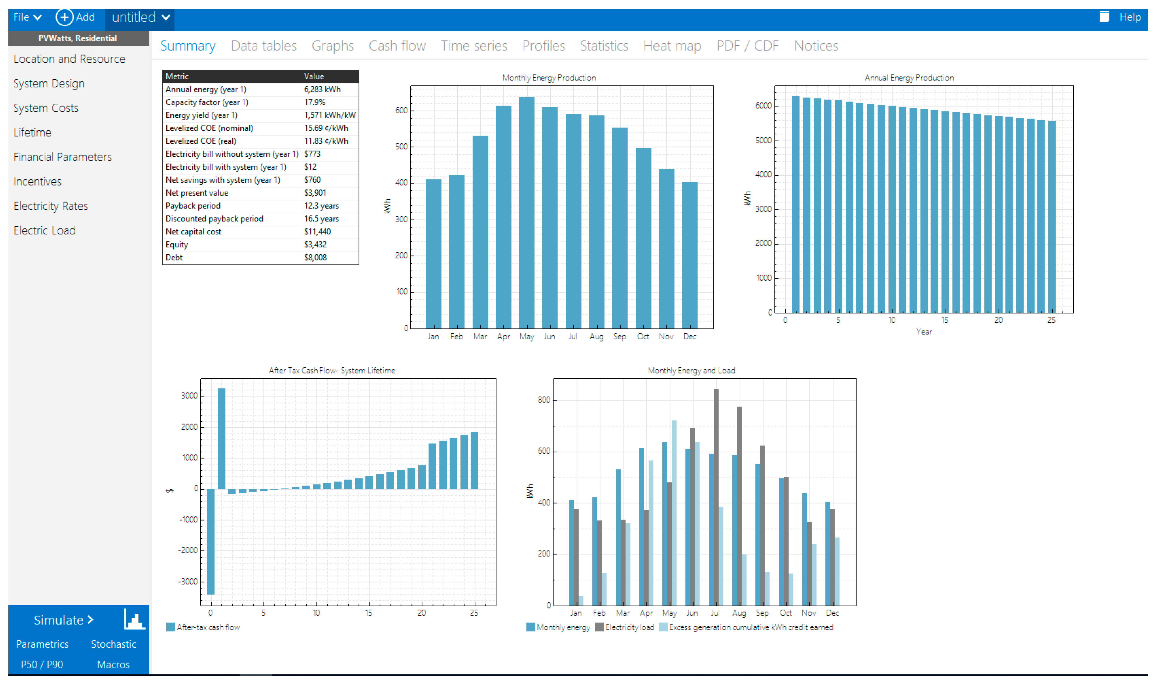
) show values of NPV = $3992, DPBT = 16.3 years, WACC = 5.4% and LCOE = 15.9 c$/kWh, while the results obtained with the SAM tool (Figure 4 and

Table 7. Results obtained for the comparison study case using SAM software.

SAM RESULTS
Economic Analysis Results		Financial Analysis Results
NPV	3901 $	WACC	5.08%
IRR	-
PI	-	Cost Analysis Results
PIM	-	LCOE	15.69 c$/kWh
DPBT	16.5 years	Cs	-

) are NPV = $3901, DPBT = 16.5 years and LCOE = 15.7 c$/kWh.

If these data are compared, certain similarities can be observed, but the added value of the procedure developed in this manuscript is its ease of use and the possibility of obtaining a very quick preliminary result, while using the SAM tool can be very time consuming for a person outside the sector due to its complexity and the technical and economic knowledge required for its proper use.

In addition, the sensitivity analysis feature included in the developed MATLAB tool is also compared with the parametric analysis available in the SAM tool.

The first setback is that contrary to the proposed tool, where you can assign discrete values of Cu, Hopt or SCI, if you want to do a sensitivity analysis with SAM, you cannot so easily change these values. For example, in order to vary the total costs of the PV system, each of the various costs that make up the total price of the system (modules, equipment, overhead, installation work, engineering, procurement, land costs, etc.) must be individually varied, which makes this sensitivity analysis more cumbersome. In the same way, it is not possible to choose arbitrary Hopt values but it is necessary to choose different locations with values similar to those proposed by the described tool.

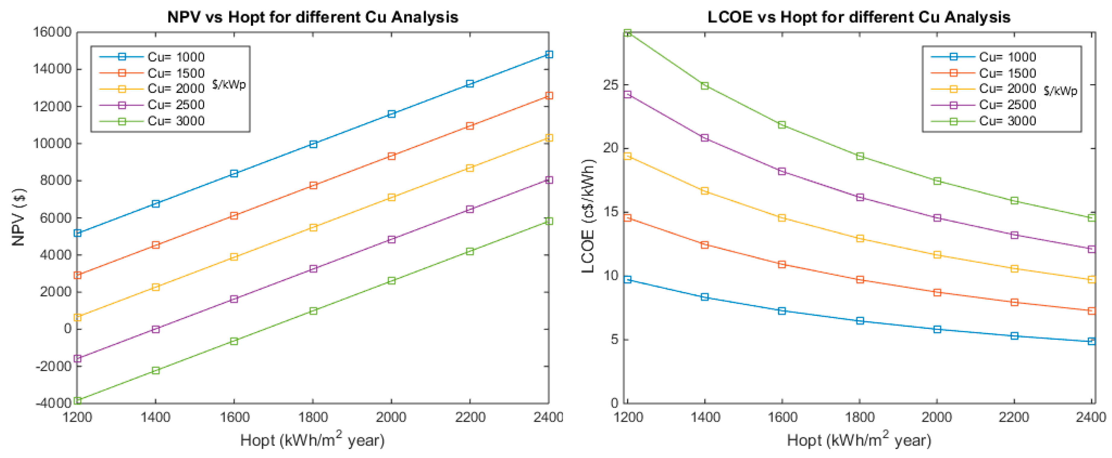
An example of two of the results obtained with the MATLAB tool can be observed in Figure 5, where the NPV and LCOE values were obtained depending on different inputs of Cu and Hopt. Besides the ease of entering discrete data from this analysis, the results are easily readable as can be observed. It should be remembered that the objective of our methodology and tool is to offer an easy means, even for a non-expert user, to obtain a preliminary overview of a possible photovoltaic investment.

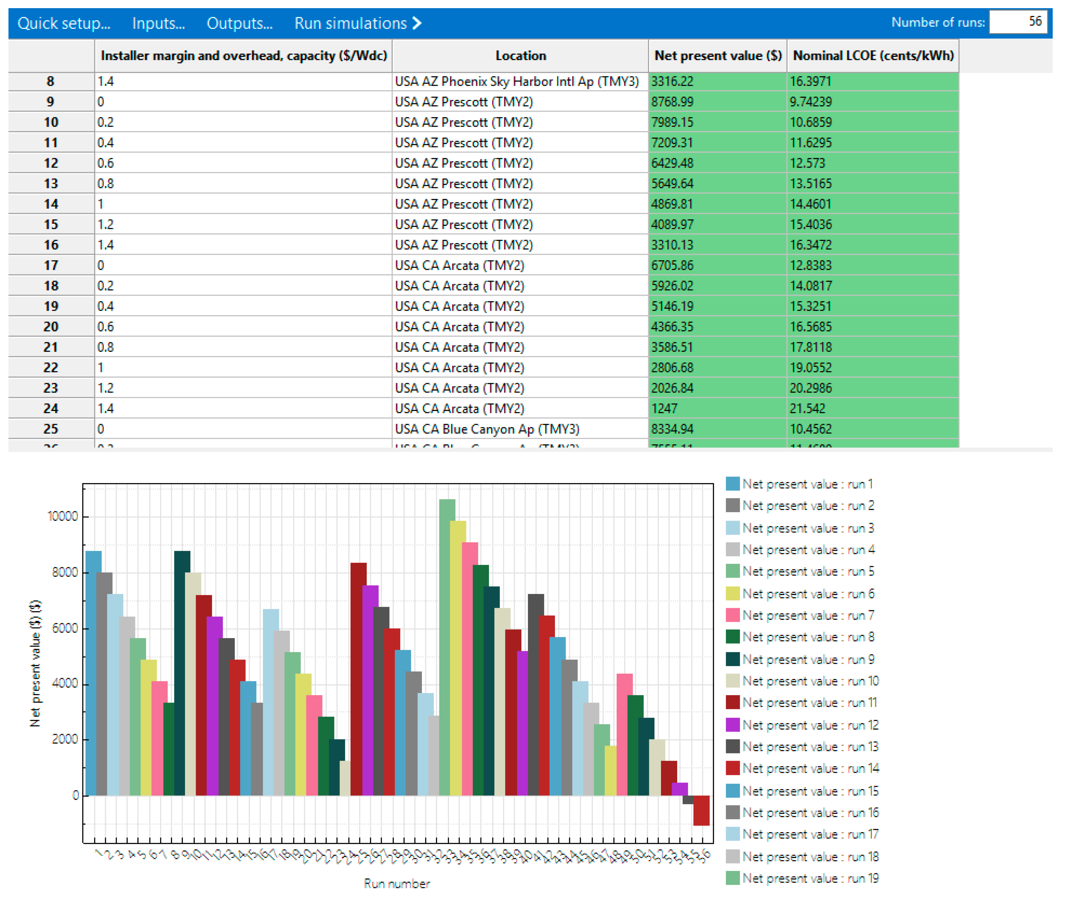
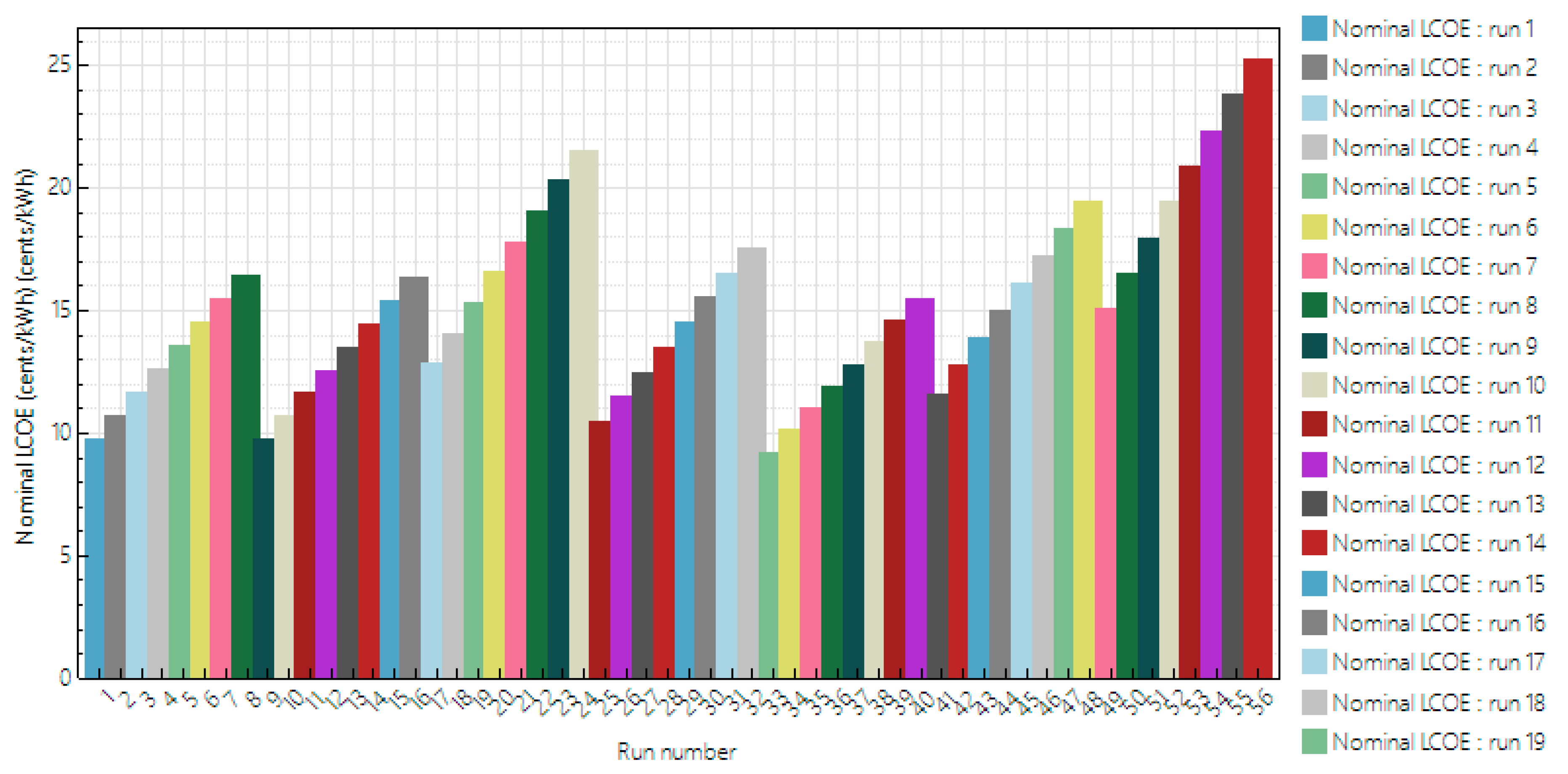
On the other hand, if one wants to transfer this same sensitivity analysis to the SAM tool, the result obtained can be seen in Figure 6 and Figure 7. Firstly, there is the complexity of entering the input data from the analysis, as mentioned above, but additionally, as observed in the result, its interpretation is more complex and requires subsequent processing of the data, which would delay having a quick preliminary idea of the feasibility of a possible investment.

Additionally, the results of the case analysis from Section 4 was compared with different papers which cover the same topic as this manuscript. It should be noted that a large number of technical, economic and financial parameters are involved in the procedure presented, and their variation depends on climate, load profile, PV system sizes, electricity price, taxes, WACC, self-consumption index, etc. Therefore, the comparison of the results of this document with those of other studies is merely indicative, as it is very difficult to compare the technical, cost, economic and finance parameters of the case studies, as well as the criteria used. However, with this comparison we want to reinforce the idea of the simplicity of the proposed methodology, without affecting its complexity or diminishing the quality of the results offered.

Table 8. Comparison study results.

Location	PV Power (kWp)	NPV (€)	IRR (%)	DPBT (yr)	PI	Reference
(Spain—Study case)	3.5	1763.3	9.8	14.2	1.4	-
Spain	5		10	12	2.13	[17]
Spain	5		8			[46]
Spain	10		6	14		[47]
Greece	4.9	1370	8.3	14.3		[21]
Germany/Ireland	6		5/6			[14]
Cyprus	4		14.6	10		[48]
Italy	3	1519		6		[15]

summarizes the study of PV systems with some parameters similar to the case described in Madrid (Spain) in Section 4.

6. Conclusions

This manuscript describes the procedure proposed for the evaluation of the economic feasibility and viability of the funding of a photovoltaic project and the calculation of the cost of its electric power generation.

Nowadays, there are numerous tools available for carrying out the profitability analysis of a photovoltaic system. However, certain shortcomings have been identified either in the definition of the economic and financial scenarios or in the results obtained, as they do not provide all the necessary information. The complexity and training requirements for the correct use of some tools means that many agents interested in the implementation of photovoltaic solutions are excluded. With the methodology that was developed and the resulting tool that was obtained, many of these identified shortcomings have been mitigated.

An important advantage of the procedure proposed, which also fills an existing gap amongst the available commercial tools, is the facility for the user to obtain the preliminary criteria that determine the economic feasibility and the financing viability, as well as the cost-competitiveness of electricity generation of any PV system. In this sense, the use of the LCOE indicator as a cost comparison tool may have certain limitations as it compares the cost of photovoltaic energy with the price of electricity in a scenario of full use of the generated energy. The novelty introduced in this article is that it takes into account the cost of direct self-consumption PV electricity (Cs) dependent on the self-consumption index (SCI).

In addition, this procedure also enables a sensitivity analysis of some of the parameters that have the greatest effect on the criteria of economic analysis, such as Internal Rate or Return, Net Present Value and Profitability Index, together with a cost-competitiveness evaluation through the Levelised Cost of Electricity. For example, it provides the evolution of LCOE as a function of H_OPT for variations of C_u, d, C_O&M, N or T.

The information provided by this procedure will be of great use for prospective owners, investors, organizations or entities interested in investing in PV systems and who need to have a preliminary decision tool to facilitate an approach to a complete PV system, no matter their level of expertise in the field. To a certain extent, it is a time-saving tool for decision making.