A Model-Based Design Approach for Stability Assessment, Control Tuning and Verification in Off-Grid Hybrid Power Plants

Abstract

This paper proposes detailed and practical guidance on applying model-based design (MBD) for voltage and frequency stability assessments, control tuning and verification of off-grid hybrid power plants (HPPs) comprising both grid-forming and grid-feeding inverter units and synchronous generation. First, the requirement specifications are defined by means of system, functional and model requirements. Secondly, a modular approach for state-space modelling of the distributed energy resources (DERs) is presented. Flexible merging of subsystems by properly defining input and output vectors is highlighted to describe the dynamics of the HPP during various operating states. Eigenvalue (EV) and participation factor (PF) analyses demonstrate the necessity of assessing small-signal stability over a wide range of operational scenarios. A sensitivity analysis shows the impact of relevant system parameters on critical EVs and enables one to finally design and tune the central HPP controller (HPPC). The rapid control prototyping and control verification stages are accomplished by means of discrete-time domain models being used in both off-line simulation studies and real-time hardware-in-the-loop (RT-HIL) testing. The outcome of this paper is targeted at off-grid HPP operators seeking to achieve a proof-of-concept on stable voltage and frequency regulation. Nonetheless, the overall methodology is applicable to on-grid HPPs, too.

1. Introduction

Off-grid electricity systems have attracted significant attention in emerging and frontier markets in order to conduct rural and island electrification and to supply remote industrial sites (e.g., mining areas) [1,2,3]. Such isolated grids—commonly associated with the microgrid (MG) concept—are characterized by increasing hybridization of the involved distributed energy resources (DERs). Traditional fossil-fueled production systems (e.g., diesel generators) are replaced or augmented by renewable generation (e.g., wind power, solar photovoltaic (PV)) and energy storage due to environmental, economic and social reasons. During the design stage of an off-grid hybrid power plant (HPP), it becomes evident that the most cost effective approach is to retain a fossil-fueled generator with time-limited operation to supply the net load demand only whenever it is needed [4,5,6,7].

It is crucial to ensure power supply and balance stability and control system stability in the HPP [8]. In this context, small-signal stability is concerned with assessing the occurrence of voltage, frequency or power oscillation modes and sufficient stability margins in every technically feasible operating state of the HPP. Moreover, a robust control solution and adequate tuning guidelines are required to keep the frequency and voltages within the operational limits.

Several publications address the topic of small-signal modeling and voltage/frequency stability assessment in MGs [9,10,11,12,13]. In [9,10] state-space models of inverters, grid and loads were developed and the sensitivities of eigenvalues (EVs) to control parameters were evaluated. The stability analysis was targeted for a MG consisting of inverter based DERs that share the grid-forming task among each other. A similar type of analysis was performed in [11] for a system with synchronous generator (SG), asynchronous generator and battery energy storage system (BESS) in PQ control mode [14]. Finally, in [12,13] the parallel operation of SG and grid-forming inverter was investigated to study the dynamics of the MG and to adjust some control parameters of the individual DERs to ensure system stability. All above-mentioned publications do not further extend their scope beyond modeling and stability analysis. Further developments and studies on control design and tuning for voltage and frequency regulation are missing which are required to achieve a proof-of-concept on the HPP control system.

In this regard, various MG control architectures are proposed in the literature and can be classified as centralized or decentralized [15,16]. However, in these publications it remains unclear how to effectively design and tune decentralized controllers with the objective of keeping the frequency and voltages within the limits during any possible operating condition. The most common way is to utilize a central system controller that dispatches commands to the individual DERs to achieve a global control objective. Here, control design and tuning methods need to take into account the dynamics occurring within the HPP. In the present literature, no clear guidelines on the models applied and control methods are identified.

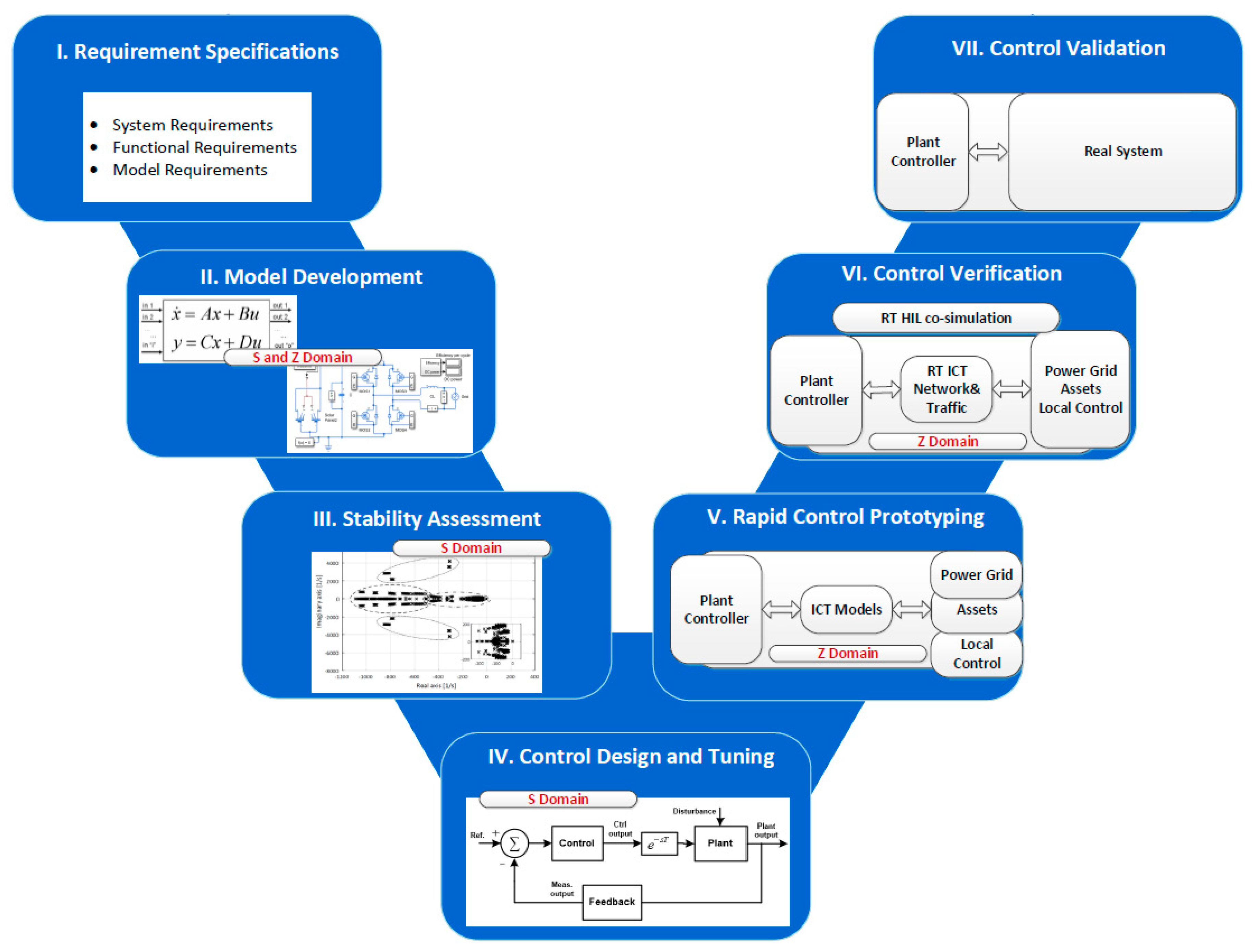
The novelty of this paper is to propose a model-based design (MBD) approach that includes all necessary building blocks to achieve stable voltage and frequency regulation in off-grid HPPs; i.e., the required set of models; a systematic and complete stability assessment; a design and tuning method of a hierarchical control system consisting of central HPP controller (HPPC) and DER controllers; and final verification and validation of the control system. The HPP in the scope of this study consists of wind turbine generator (WTG), PV, BESS and a fossil-fuel generator set (hereinafter called genset). An overview of the different stages from development to testing is given in Figure 1.

Section 2 describes the requirement specifications which are distinguished into system, functional and modeling requirements (Step I).

In Section 3, a modular approach for state-space modelling of each DER, and subsequently the entire HPP is presented (Step II). State-of-the-art inverter models and generic rules for control design are referenced. The state, input and output vectors of the state-space models are summarized. A representative model of the genset including speed governor and automatic voltage regulator (AVR) is summarized in equal manner. Here, it is highlighted how to utilize in and output variables of the model depending on whether grid-forming inverter and/or genset provide the grid frequency reference. A set of numerical simulation models is proposed to be used during the rapid control prototyping (RCP) and control verification stage.

In Section 4 a voltage and frequency stability assessment is shown (Step III). First, EV and participation factor (PF) analysis was conducted for two relevant test scenarios; i.e., genset in or out of service. The occurring dynamic modes and the associated state variables of each DER were clustered with respect to their eigenfrequencies. Such a clustering method provides insight into the dynamic modes and control parameters that require further attention with regard to absolute and relative system stability. Subsequently, the sensitivity of EVs to certain DER control parameters was assessed. This is a useful step to gain more confidence on specific control parameters (e.g., droop gains) which need to be parametrized in the context of the entire HPP.

Section 5 deals with the design and tuning of voltage and frequency controller (Step IV). State-space models are converted to transfer functions which are used to tune DER control parameters and design and tune the central HPPC.

Subsequently Section 6 shows discrete-time domain models being applied to test the control algorithms under various operating conditions to identify the robustness of the design (Step V). This stage is called RCP.

The final stage of proposed MBD approach is control verification and validation against system and functional requirements (Step VI and VII). In Section 7, an outlook is given for verifying the performance of HPPC platform by means of real-time hardware-in-the-loop (RT-HIL) testing. The developed control algorithms including physical implementation on target hardware are then ready for site testing as a final validation stage.

The mathematical formulations and procedures are demonstrated in general to enable studies in off-grid HPPs on either kW-scale or MW-scale and with modular expansion of the production subsystem.

2. Step I: Requirement Specifications

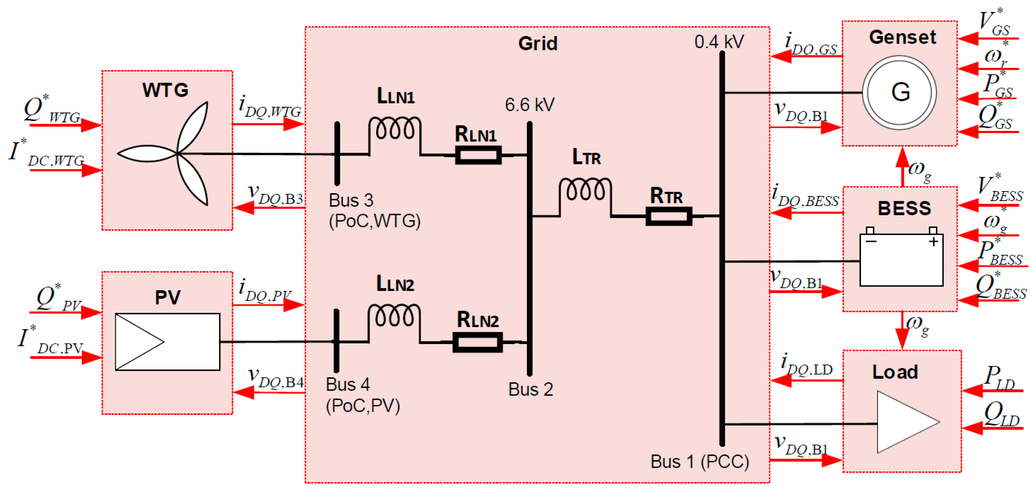
The single-line diagram (SLD) of the benchmark off-grid HPP investigated in this study is shown in Figure 2.

This paper uses the optimal configuration for an off-grid HPP, as derived in [3], since it constitutes a representative system optimized from a techno-economic perspective. The production subsystem consists of a full-scale converter WTG (80 kW) and PV (40 kW), a BESS (160 kWh/90 kVA) and a fossil-fuel genset (90 kVA). At least one grid-forming unit is required that provides the voltage and frequency reference in the HPP. Typically, SGs are responsible for this task. By allowing flexible HPP operation with partial shut-down of fossil-fuel generators it becomes evident that the BESS inverter system must implement grid-forming capabilities, too. Then, it is not desirable to switch between various control schemes, since it prevents smooth transition due to controller reset and eventual plant shut-down and restart. Hence, the optimum solution for the power management strategy is to use droop regulation. It ensures seamless transition between operation scenarios on the one hand, and on the other facilitates smoother integration of the HPP, if it becomes grid-connected.

The demand subsystem (90 kW peak) might comprise multiple low voltage (LV) feeders with residential, commercial and small industrial consumers. In this study, it is represented as an aggregated electrical load which is modelled as constant impedance (RL) load [17]. Production and demand subsystems are connected via the point of common coupling (PCC).

2.1. Step Ia: Defining System Requirements

System requirements are related to the performance of the HPP system and are usually specified in so-called grid codes, technical regulations or guidelines.

First and foremost, it is essential in off-grid HPPs to ensure system stability for voltage and frequency regulation due to the characteristics of isolated MGs. The stability phenomena in MGs, which can be classified as control system stability and power supply and balance stability, are explained in [8] and summarized in [18]. Absolute and relative stability can be measured by means of an EV analysis. Absolute stability is ensured if all poles are located in the left half plane. Relative stability is associated with the damping ratio of the EVs. In order to avoid critically low damping of any voltage or frequency oscillations in the HPP, a reasonable target for the damping ratio is $\zeta \ge 0.05$ according to [19].

Then, operational requirements for off-grid HPPs are difficult to define by means of existing grid codes, since each MG size, the layout, the DERs involved, and hence, the related technical regulations, are unique [18]. However, some generic guidelines are found in [20]. A steady-state voltage and frequency profile of $f_g=\left\{48,52\right\} \mathrm{Hz}$ and $V=\left\{0.85,1.15\right\} \mathrm{pu}$ is suggested. Dynamic performance requirements for voltage and frequency regulation are not specified.

2.2. Step Ib: Defining Functional Requirements

Functional requirements refer to the necessary functions that are to be implemented in the HPP control system in order to satisfy certain system requirements. A comprehensive overview of the required control functions in MGs is provided in [21] and summarized in [18]. In this section, the specific elements of voltage and frequency control function are elaborated on.

As explained previously in this section one part of the overall power management strategy is to utilize parallel grid-forming DERs (i.e., BESS and genset) to regulate grid frequency and voltages within their nominal limits specified in Section 2.1. Moreover, the studies in [13] reveal that it is important to evaluate the transient power sharing performance between several grid-forming units—to avoid any unwanted oscillations within the HPP and to minimize the duration of unequal power sharing. This aspect is related to DER droop regulation (primary control) [13]. Primary control actions by DERs will leave steady-state errors in voltage and frequency. There are good reasons that these deviations from the nominal value should be eliminated, even if the voltages and frequency remain within the normal operating range. Firstly, it is not desired to operate the PCC voltage below nominal value, as it will lower the voltage levels in the demand subsystem as well. Depending on the feeder length and the connected loads, severe undervoltages can be expected that would lead to load disconnection. Secondly, it is preferred to avoid grid frequencies below nominal value for a longer time period, as they will lower the power consumption and efficiency of some frequency dependent loads; e.g., hydraulic pumps. Field measurements in an island power system with water supply pumps have revealed that the active load changes with approximately 8.5%/Hz [22]. Hence, steady-state voltage and frequency errors need to be compensated by secondary control actions of the central HPPC.

2.3. Step Ic: Defining Modeling Requirements

As part of the MBD process it is necessary to define certain requirements of the models being developed in Step II:

• Linearized models are required for stability assessment and control tuning in frequency domain.
• The model bandwidth shall be limited to a minimum value that enables the assessment of voltage and frequency stability and control.
• Numerical models are required that are applicable for RCP and control verification purposes. Computational effort of model execution shall be taken into account to achieve accelerated off-line simulation studies during RCP stage and to ensure real-time capability for RT-HIL testing.
• Simulation platforms must be carefully selected to reduce the modeling effort by re-using developed models throughout various MBD stages shown in Figure 1.

3. Step II: Modeling of Hybrid Power Plant

3.1. Step IIa: Modeling Plant Components in State-Space

The small-signal models were developed using the state-space approach, as it allows one to represent each plant component separately and subsequently merge according to the balance of plant (BoP) shown in Figure 2 [18]. With regard to stability analysis, any unstable system mode can be consistently assessed by means of frequency and damping ratio (EV analysis) and ascribed to the causative state variables (PF analysis). Furthermore, state-space models can be directly converted to transfer functions, and thus applied in the control tuning stage [18]. It is possible to develop state-space models in either S-domain or Z-domain. However, since the dynamics in the power system applications involve a wide range of time constants and various sampling times for the involved subsystems, a continuous time domain tuning is preferred. Some considerations on the required level of model details for assessing voltage and frequency stability are given in [18]. It should be noted that the models described do not facilitate harmonic stability assessment and are solely be used for voltage and frequency stability assessment and control design and verification.

A set of state-space equations describe dynamic states of the system. The linearized differential equations of each plant component model are obtained by linearizing around steady-state values with resulting matrices A, B and C; D linking state vector x; input vector u; and output vector y according to Equation (1) [23].

$$\begin{array}{c}\Delta \frac{\mathit{d}\mathit{x}}{\mathit{d}\mathit{t}}=\mathit{A}\Delta \mathit{x}+\mathit{B}\Delta \mathit{u} \\ \Delta \mathit{y}=\mathit{C}\Delta \mathit{x}+\mathit{D}\Delta \mathit{u}.\end{array}$$

(1)

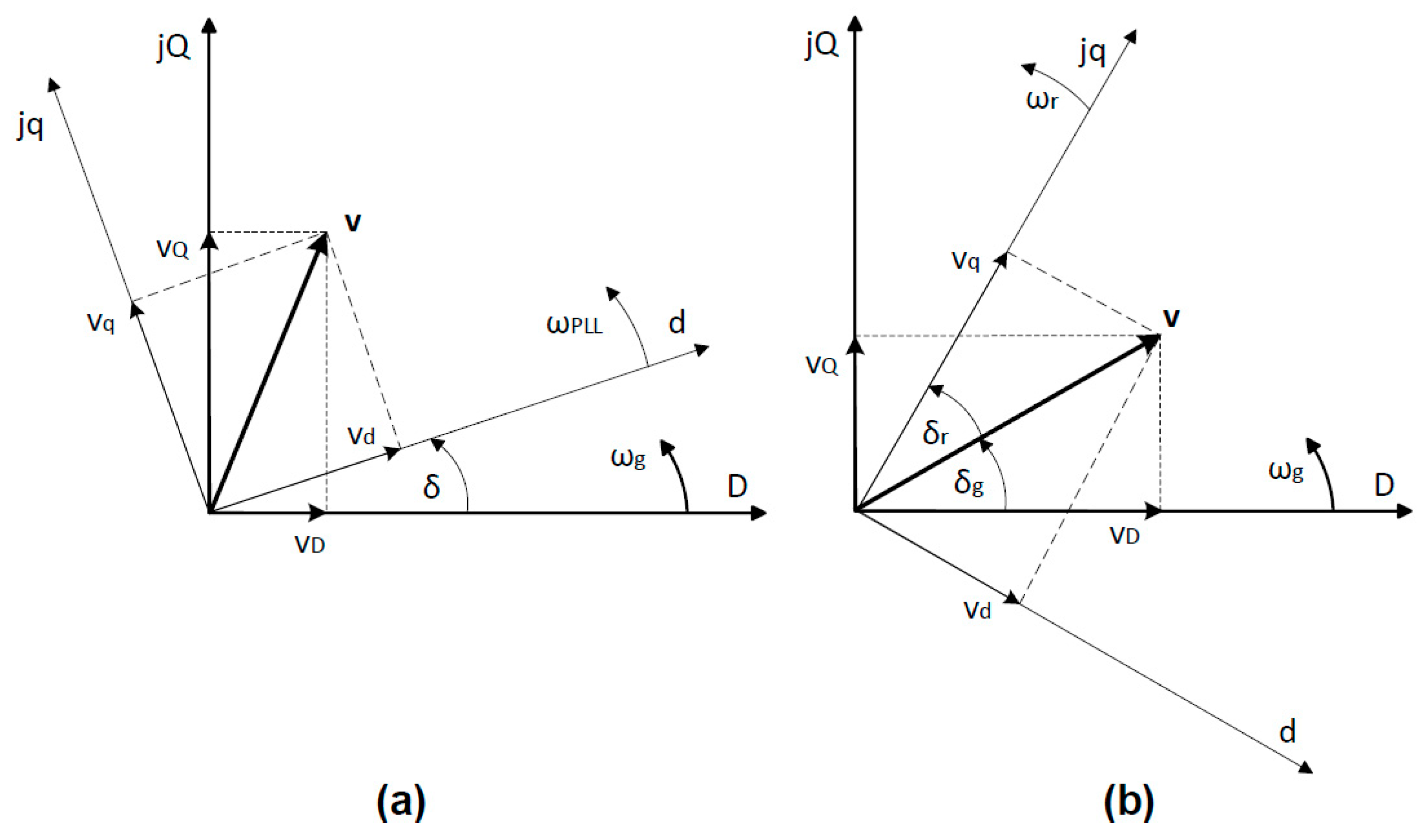
Each plant component model presented in this section is represented in a local synchronous rotating reference frame (SRRF) with dq-variables. The global reference frame (DQ-variables) of the HPP model is defined on the grid rotating at angular frequency ${\mathit{\omega }}_{\mathit{g}}$. Equations (2) and (3) describe the Park transformation of reference frames. The matrix in Equation (3) is valid for inverter based units where the local SRRF is aligned with the d-axis grid voltage $v_d$ and grid voltage angle ${\delta }_g$ (Figure 3a). In case of the genset the local SRRF rotates at rotor speed ${\omega }_r$ and is aligned with the q-axis voltage $v_q$ and rotor angle ${\delta }_r$ as expressed by Equation (4). and illustrated in Figure 3b.

$$\left[\begin{array}{c}{v}_d\\ v_q\end{array}\right]=\left[T\right]\left[\begin{array}{c}{v}_D\\ v_Q\end{array}\right]$$

(2)

$$T_{PES}=\left[\begin{array}{cc}\cos {\delta }_g& \sin {\delta }_g\\ -\sin {\delta }_g& \cos {\delta }_g\end{array}\right]$$

(3)

$$T_{GS}=\left[\begin{array}{cc}\sin ({\delta }_g+{\delta }_r)& -\cos \left({\delta }_g+{\delta }_r\right)\\ \cos \left({\delta }_g+{\delta }_r\right)& \sin \left({\delta }_g+{\delta }_r\right)\end{array}\right]$$

(4)

The correct performance of linearized state-space models has been verified in MATLAB SimPowerSystems Toolbox by means of numerical models which are described in Section 3.3.

In the following subsections, the state-, input- and output vectors of each component state-space model are explained as they are of high relevance for the EV and PF analysis. The corresponding system matrices can be found in various references [17,24,25,26,27].

3.1.1. Grid-Forming Inverter

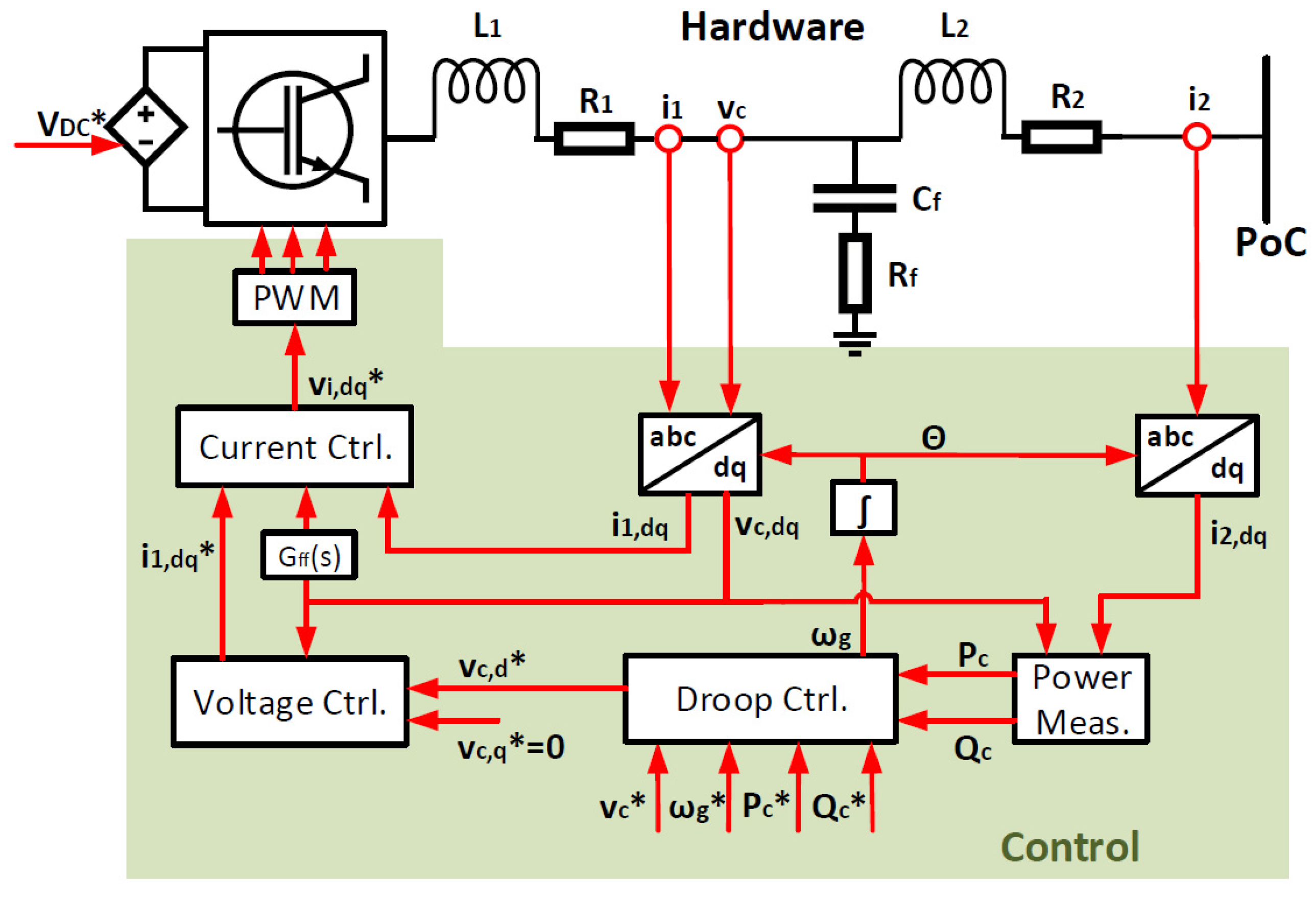
In Figure 4 the most typical structure of a grid-forming inverter with droop control mechanism and power-based synchronization is depicted. It is characterized by an ideal voltage source with low output impedance [14]. The grid-forming functionality can be part of the BESS, where the voltage is controlled by a DC/DC converter at the source side. The dynamic model of the grid-forming inverter is explained in [13] and [28] and serves as a basis for the subsequent state-space representation.

The state vector ${\mathit{x}}_{\mathit{F}\mathit{O}\mathit{R}\mathit{M}}$ of the small-signal model is given by Equation (5) where:

• $i_{1d}$, $i_{1q}$, $i_{2d}$, $i_{2q}$, $v_{cd}$ and $v_{cq}$ refer to the dynamic states of LCL filter. Note that it is necessary to represent the filter capacitance, as the voltage $v_c$ is controlled in this control structure.
• ${\phi }_{id}$ and ${\phi }_{iq}$ are the state variables of the current controller (PI).
• ${\phi }_{vcd}$ and ${\phi }_{vcq}$ are the state variables of the outer voltage controller of type PI.
• $P_{c,avg}$ and $Q_{c,avg}$ refer to the dynamics of a low pass filter (LPF) for power measurements, leading to an average value for active and reactive power.

  $${\mathit{x}}_{\mathit{F}\mathit{O}\mathit{R}\mathit{M}}=\left[\begin{array}{ccc}{i}_{1d}& i_{1q}& i_{2d}\end{array} \begin{array}{ccc}{i}_{2q}& v_{cd}& v_{cq}\end{array} \begin{array}{ccc}{\phi }_{id}& {\phi }_{iq}& {\phi }_{vcd}\end{array} \begin{array}{ccc}{\phi }_{vcq}& P_{c,avg}& Q_{c,avg}\end{array}\right]$$

  (5)

The classic droop characteristics for active power sharing (${\omega }_g/P_c$) and reactive power sharing ($v_c/Q_c$) can be used, since the coupling impedance between grid-forming inverter and genset is mainly given by the grid-side inductor of the inverter ($X\gg R$). The essential components for the implementation of droop control are the LPF cut-off frequency $f_{LPF,PQ}$ applied for the power-based synchronization (Equation (6)) and the droop characteristics. They need to be parametrized in the context of the entire HPP to ensure stable operation in parallel to other grid-supporting DERs, as demonstrated later in Section 4 and Section 5.

$$\left[\begin{array}{c}\frac{d{P}_{c,avg}}{dt}\\ \frac{d{Q}_{c,avg}}{dt}\end{array}\right]=2\pi \cdot f_{LPF,PQ}\cdot \langle \left[\begin{array}{c}{P}_c\\ Q_c\end{array}\right]-\left[\begin{array}{c}{P}_{c,avg}\\ Q_{c,avg}\end{array}\right]\rangle$$

(6)

It is defined that the grid-forming inverter provides the global reference frame to be used by the remaining HPP component models, in this way $d=D$, $q=Q$.

The input vector ${\mathit{u}}_{\mathit{F}\mathit{O}\mathit{R}\mathit{M}}$ is defined in Equation (7), where grid voltage variables $v_{gD}$ and $v_{gQ}$, voltage reference $V_c^{*}$, frequency reference ${\omega }_g^{*}$, active power reference $P_c^{*}$ and reactive power reference $Q_c^{*}$ act as input variables to the system.

$${\mathit{u}}_{\mathit{F}\mathit{O}\mathit{R}\mathit{M}}=\left[\begin{array}{cc}{v}_{gD}& v_{gQ}\end{array} \begin{array}{cc}{V}_c^{*}& {\omega }_g^{*}\end{array} \begin{array}{cc}{P}_c^{*}& Q_c^{*}\end{array}\right]$$

(7)

The output vector ${\mathit{y}}_{\mathit{F}\mathit{O}\mathit{R}\mathit{M}}$ provides the currents $i_{2D}$ and $i_{2Q}$ at the PoC and the grid frequency ${\omega }_g$ (Equation (8)).

$${\mathit{y}}_{\mathit{F}\mathit{O}\mathit{R}\mathit{M}}=\left[\begin{array}{ccc}{i}_{2D}& i_{2Q}& {\omega }_g\end{array}\right]$$

(8)

Again, the power-electronic switches are not modeled explicitly, as their dynamic process is in the kHz range, and thus, not relevant for voltage and frequency control.

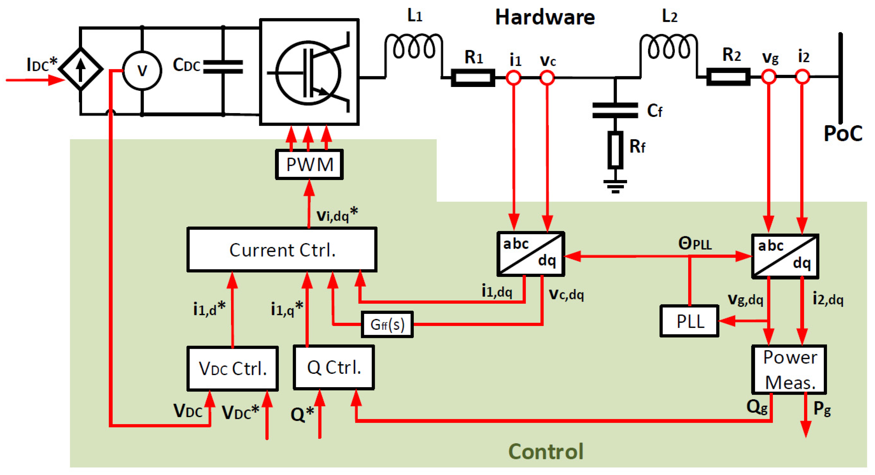
3.1.2. Grid-Feeding Inverter

Figure 5 shows a schematic diagram of a grid-feeding inverter which is characterized by a current-controlled source connected to the grid with high parallel impedance [14]. It is the most typical inverter control structure of grid-connected WTGs and PV systems [29]. The dynamics of the DER source side are not considered due to the decoupling effect of the inverter DC link. A comprehensive overview on the modeling and control design of a grid-feeding inverter is provided in [13] and [28] and was used in this study.

Vector ${\mathit{x}}_{\mathit{F}\mathit{E}\mathit{E}\mathit{D}}$ (Equation (9)) describes the dynamic state variables of the system where:

• The dynamic states of LCL filter and current controller are the same as in grid-forming control mode. Note that it is not mandatory to represent the filter capacitance for the intended studies in this paper, as harmonics are not of concern. It is nevertheless retained to align the modeling representation of grid-forming and grid-feeding inverter control structure.
• ${\phi }_{vdc}$ and ${\phi }_{Qg}$ relate to the PI controllers of DC link voltage and reactive power respectively.
• $V_{dc}$ corresponds to the dynamic of DC-link capacitor and $Q_{g,avg}$ to a LPF for reactive power measurement.
• ${\phi }_{PLL}$ belongs to a first-order filter of the phase-locked loop (PLL) and $\delta$ is the phase angle dynamic as a derivative of the grid frequency.

  $${\mathit{x}}_{\mathit{F}\mathit{E}\mathit{E}\mathit{D}}=\left[\begin{array}{ccc}{i}_{1d}& i_{1q}& i_{2d}\end{array} \begin{array}{ccc}{i}_{2q}& v_{cd}& v_{cq}\end{array} \begin{array}{ccc}{\phi }_{id}& {\phi }_{iq}& {\phi }_{vdc}\end{array} \begin{array}{ccc}{\phi }_{Qg}& V_{dc}& Q_{g,avg}\end{array} \begin{array}{cc}{\phi }_{PLL}& \delta \end{array}\right]$$

  (9)

The input vector ${\mathit{u}}_{\mathit{F}\mathit{E}\mathit{E}\mathit{D}}$ is defined in Equation (10), where the grid voltage variables $v_{gD}$ and $v_{gQ}$, the reactive power reference $Q_g^{*}$ and the DC source current $I_{dc}^{*}$ act as input variables to the system. $I_{dc}^{*}$ represents an active power modulation of the WTG or PV system.

$${\mathit{u}}_{\mathit{F}\mathit{E}\mathit{E}\mathit{D}}=\left[\begin{array}{cc}{v}_{gD}& v_{gQ}\end{array} \begin{array}{cc}{Q}_g^{*}& I_{dc}^{*}\end{array}\right] .$$

(10)

The output vector ${\mathit{y}}_{\mathit{F}\mathit{E}\mathit{E}\mathit{D}}$ of the system (Equation (11)) provides the currents $i_{2D}$ and $i_{2Q}$ at the point of connection (PoC).

$${\mathit{y}}_{\mathit{F}\mathit{E}\mathit{E}\mathit{D}}=\left[ \begin{array}{cc}{i}_{2D}& i_{2Q}\end{array}\right] .$$

(11)

It should be noted that an average model of the inverter is used to represent the pulse width modulation (PWM) of power-electronic switches, assuming that $v_{i,dq}=v_{i,dq}^{*}$ (Figure 5). This type of model preserves the average voltage dynamics over one fundamental period being necessary to design controls [8].

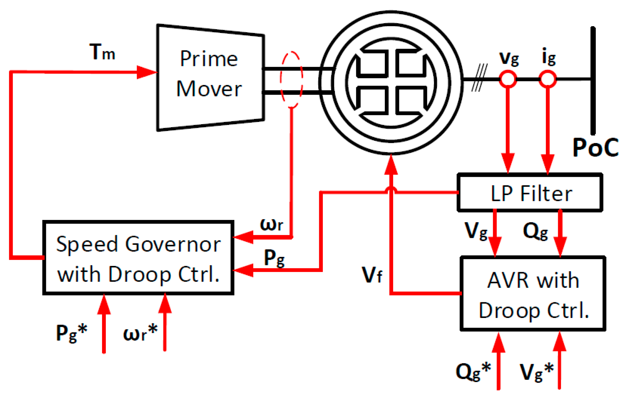
3.1.3. Generator Set

Figure 6 shows a schematic diagram of a genset with speed-governor droop and AVR droop function. The genset model consists of three main elements; i.e., electrically excited SG, speed governor and AVR. The SG is described by a 7th-order model including stator and rotor flux linkage dynamics and rotor dynamics [26]. The dynamics of prime mover and excitation system are modeled as a simple first-order time response [13,27]. Speed governor and AVR are implemented by a PID controller with design specifications given in [13].

The resulting state-space model of the entire genset is characterized by its state vector ${\mathit{x}}_{\mathit{G}\mathit{S}}$ in Equation (12) where:

$${\mathit{x}}_{\mathit{G}\mathit{S}}=\left[\begin{array}{c}\begin{array}{ccc}{i}_{gd}& i_{fd}& i_{kd}\end{array} \begin{array}{ccc}{i}_{gq}& i_{kq}& {\omega }_r\end{array} \begin{array}{cc}{\delta }_r& P_{g,avg}\end{array}\\ \begin{array}{ccc}{Q}_{g,avg}& v_{g,avg}& {\phi }_{G1}\end{array} \begin{array}{ccc}{\phi }_{G2}& T_m& {\phi }_{AVR1}\end{array} \begin{array}{cc}{\phi }_{AVR2}& v_{fd}\end{array}\end{array}\right]$$

(12)

• The first five state variables result from the stator and rotor flux dynamics. $i_{gd}$ and $i_{gq}$ are the stator currents, $i_{kd}$ and $i_{kq}$ are currents in the damper winding and $i_{fd}$ is the field winding current [26].
• The rotor dynamics are expressed by the swing equation (Equation (13)). It should be noted that $\Delta {\omega }_r$ is the rotor angular speed deviation from the grid angular frequency. $H$ is the inertia time constant, $D$ the damping factor coefficient and $T_m$ and $T_e$ the mechanical and electrical torques. An expression for the rotor angle displacement $\Delta {\delta }_r$ is given in Equation (14) [30].

  $$H\frac{d\Delta {\omega }_r}{dt}=T_m-T_e-D\cdot \Delta {\omega }_r=T_m-T_e-D\cdot \left({\omega }_r-{\omega }_g\right)$$

  (13)

  $$\frac{d\Delta {\delta }_r}{dt}=\Delta {\omega }_r={\omega }_r-{\omega }_g$$

  (14)
• $P_{g,avg}$, $Q_{g,avg}$ and $v_{g,avg}$ refer to the dynamics of a LPF for voltage and current measurement, leading to an average value for active and reactive power.
• ${\phi }_{G1}$ and ${\phi }_{G2}$ are the derivative and integral states of the governor PID controller, while $T_m$ relates to the change in mechanical torque due to prime mover dynamics (fuel actuator and combustion engine).
• ${\phi }_{AVR1}$ and ${\phi }_{AVR2}$ are the derivative and integral states of the AVR, while $v_{fd}$ corresponds to the dynamics of the excitation voltage.

Droop characteristics are implemented for both speed governor (${\omega }_r/P_g$) and AVR ($v_g/Q_g$).

The input vector ${\mathit{u}}_{\mathit{G}\mathit{S}}$ is given in Equation (15), where grid voltage variables $v_{gD}$ and $v_{gQ}$, voltage reference $V_g^{*}$, speed reference ${\omega }_r^{*}$, active power reference $P_g^{*}$ and reactive power reference $Q_g^{*}$ act as input variables to the system. It should be noted that the grid frequency ${\omega }_g$, imposed by the grid-forming inverter, is an input variable as well.

$${\mathit{u}}_{\mathit{G}\mathit{S}}=\left[\begin{array}{cc}{v}_{gD}& v_{gQ}\end{array} \begin{array}{cc}{\omega }_r^{*}& P_g^{*}\end{array} \begin{array}{ccc}{V}_g^{*}& Q_g^{*}& {\omega }_g\end{array}\right]$$

(15)

The output vector ${\mathit{y}}_{\mathit{G}\mathit{S}}$ (Equation (16)) involves the currents $i_{gD}$ and $i_{gQ}$ at the generator terminals and the rotor speed ${\omega }_r$.

$${\mathit{y}}_{\mathit{G}\mathit{S}}=\left[\begin{array}{ccc}{i}_{gD}& i_{gQ}& {\omega }_r\end{array}\right]$$

(16)

In cases when a grid-forming inverter is absent, ${\omega }_g$ is not an input variable any longer. In this case, the rotor speed becomes synchronized with the grid frequency (${\omega }_r={\omega }_g$).

3.2. Step IIb: Merging of State-Space Models

The remaining components of the HPP are distribution lines, transformers and loads. The corresponding state-space expressions are well-known and can be found in [17].

Subsequently, all grid components and the individual DER state-space models need to be connected according to BoP shown in Figure 2 (black colored). This is achieved by linking input and output variables of the models in the global SRRF, as indicated by the functional diagram in Figure 2 (red colored). As a result a multiple-input-multiple-output (MIMO) model with matrices ${\mathit{A}}_{\mathit{H}\mathit{P}\mathit{P}}$, ${\mathit{B}}_{\mathit{H}\mathit{P}\mathit{P}}$, ${\mathit{C}}_{\mathit{H}\mathit{P}\mathit{P}}$ and ${\mathit{D}}_{\mathit{H}\mathit{P}\mathit{P}}$ is obtained [18].

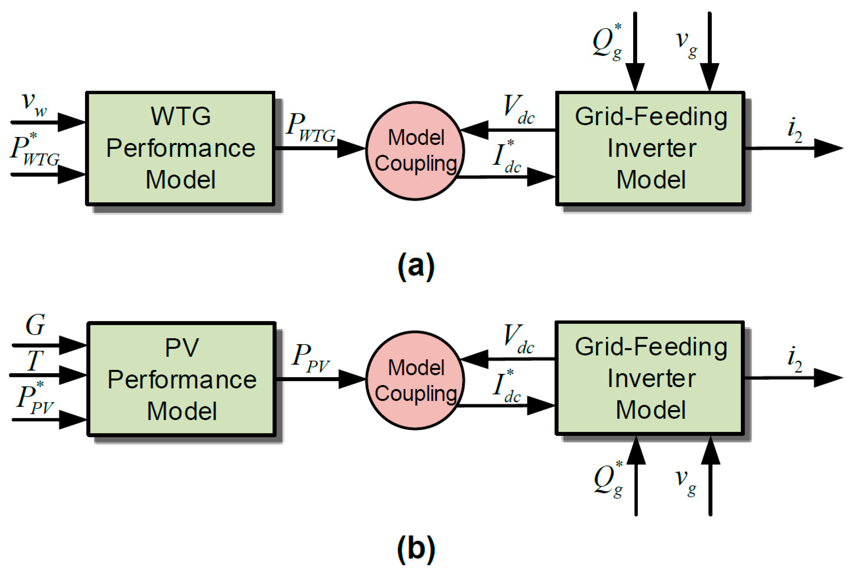
3.3. Step IIc: Developing Discrete-Time Domain Models for Control Verification

So far, linearized state space models have been developed in the S-domain for the purpose of small-signal analysis and controller tuning. At this stage, it was proposed to prepare in parallel numerical simulation models that, on the one hand, can validate the developed small-signal models, and on the other hand, can be used later on for RCP (Step V) and control verification (Step VI). Here, dynamic models of WTG, PV, BESS and genset were to be implemented by means of discrete-time domain models [31]. Thus, they can be used both for accelerated off-line simulation studies and for RT-HIL verification, as explained in Section 1.

The grid-forming inverter model described in Section 3.2 does sufficiently represent the dynamic behavior of BESSs. The transient response for voltage and frequency control is dominated by the inverter system, while the voltage/current dynamics of the battery cells can be neglected ($V_{DC}^{*}=const.$; see Figure 4) [31].

With regards to WTG and PV system, it is necessary to further extend the model capabilities beyond the inverter system in order to conduct realistic test scenarios for control assessment. More specifically, DC current variations are expected due to changes in power ($I_{DC}^{*}\ne const.$; see Figure 5). Some simple performance models of WTG and PV are proposed and validated by field data in [31]. They are capable of emulating power output variations according to wind speed $v_w$, solar irradiance $G$, temperature $T$ and active power reference $P_{WTG}^{*}$ or $P_{PV}^{*}$, respectively. Figure 7 shows how the inverter models described in Section 3.2 are coupled with the performance models proposed in [31]. $P_{WTG}$ and $P_{PV}$ are AC power output at the DER’s PoC. Hence, the model coupling block accounts for inverter and possible transformer losses and calculates the DC current input to the inverter model by using the generated DC power $P_{DER,dc}$ of each DER, respectively (Equation (17)).

$$I_{DC}^{*}=\frac{P_{DER,dc}}{V_{dc}}$$

(17)

Input and output signals of the grid-feeding inverter model are as described in Figure 5.

4. Voltage and Frequency Stability Assessment

This section deals with the assessment of voltage and frequency stability by using the state-space models described in Section 3.1 and 3.2.

4.1. Step IIIa: Defining Relevant Operating Sccenarios

The EVs of state matrix ${\mathit{A}}_{\mathit{H}\mathit{P}\mathit{P}}$ were determined for two essential operational scenarios of the HPP [3]: (1) only grid-forming inverters (i.e., BESS) and grid-feeding inverters (i.e., WTG, PV) are in operation; (2) all inverter based DERs and genset are in operation. For each scenario, matrix ${\mathit{A}}_{\mathit{H}\mathit{P}\mathit{P}}$ is updated by model linearization around steady-state values, which are within the range of normal operating conditions; i.e., $V_g=\left\{0.85,1.15\right\}\mathrm{pu}$, $f_g=\left\{48,52\right\}$ Hz, $P_{LD}=\left\{0,1\right\}\mathrm{pu}$, $P_{WTG}=\left\{0,1\right\}\mathrm{pu}$, $P_{PV}=\left\{0,1\right\}\mathrm{pu}$. In this way, a thorough stability assessment is assured as the system behavior might depend on its actual operating state, i.e., permitted voltage and frequency deviations [20], and partial or full loading of DERs.

The EVs represent dynamic modes of the HPP system and are characterized by its frequency and damping ratio. Then, in order to identify the dominant state variables participating in a particular dynamic mode, it is necessary to determine the participation matrix $P_i$. Its PFs $p_{ki}$ are obtained by Equation (18), where the right (${\varphi }_{ki}$) and left (${\psi }_{ki}$) eigenvectors of the system matrix ${\mathit{A}}_{\mathit{H}\mathit{P}\mathit{P}}$ are used. The magnitudes of $p_{ki}$ provide a measure of the relative participation of the kth state variable in the ith mode and vice versa. [23]

$$P_i=\left[\begin{array}{c}\begin{array}{c}{p}_{1i}\\ p_{2i}\end{array}\\ \begin{array}{c}⋮\\ p_{ni}\end{array}\end{array}\right]=\left[\begin{array}{cc}\begin{array}{c}{\varphi }_{1i}\\ {\varphi }_{2i}\end{array}& \begin{array}{c}{\psi }_{1i}\\ {\psi }_{i2}\end{array}\\ \begin{array}{c}⋮\\ {\varphi }_{ni}\end{array}& \begin{array}{c}⋮\\ {\psi }_{in}\end{array}\end{array}\right]$$

(18)

In both test scenarios, the cut-off frequency for the grid-forming inverter’s power measurement filter is per default $f_{LPF,PQ}=5 \mathrm{Hz}$ according to [13]. The droop characteristics are set to 5% for both frequency/active power control and voltage/reactive power control.

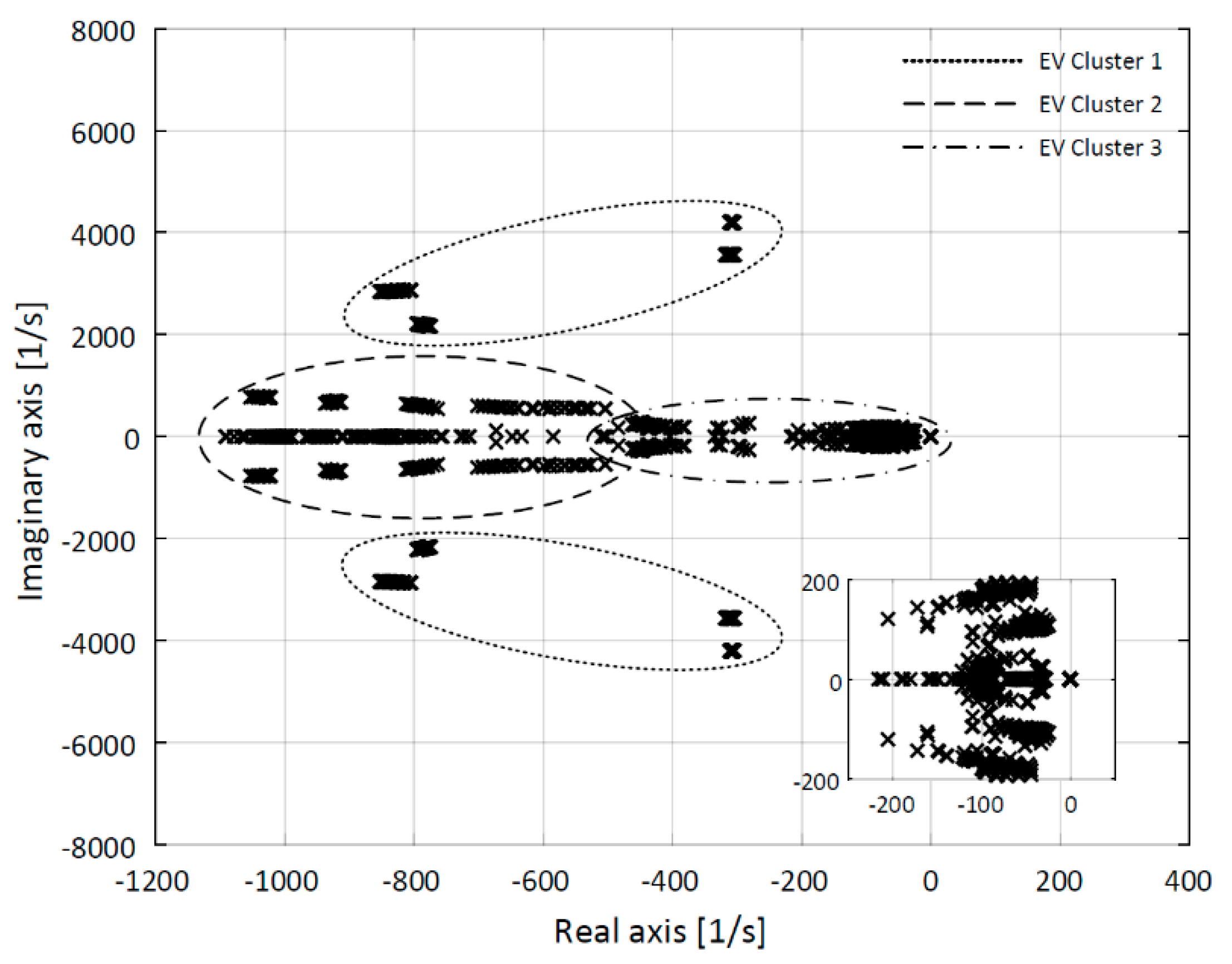
4.2. Step IIIb: Clustering of Eigenvalues

Figure 8a shows the EV map for HPP operation with only grid-forming and grid-feeding inverters. It was ascertained that all poles were located in the left hand side of the complex plane, indicating that the plant model is stable. The distribution of EVs demonstrates that their location depends on the linearization points. A detailed analysis of EV movement was not attempted due to the vast number of dynamic modes. Instead, the focus of this analysis was to determine absolute stability by identifying EVs in the right-half plane and relative stability by observing the EVs with lowest damping ratio.

In order to illustrate the extensive results of EV and PF analysis more effectively, a clustering of EVs was attempted.

Table 1. Clustering of eigenvalues for test scenario 1.

EV Cluster	Eigenfrequency ${\mathit{f}}_{\mathit{n}}$ [Hz]	Damping Ratio $\mathit{\zeta }$ [-]	Associated Dominant State Variables
1	{185, 20 × 103}	{0.03, 0.79}	Plant inductances and capacitances
2	{130, 160}	1	Inverter inner current control loops
3	{5, 30}	{0.39, 1}	Inverter outer control loops

presents several clusters of EVs according to their eigenfrequencies and associated state variables. The identified EV clusters are encircled in Figure 8.

Cluster #1 involves the time constants of physical plant parameters; i.e., inductances and capacitances of inverter LCL filters and DC link, plant transformers and distribution lines. Some EVs are highly underdamped ($\zeta =0.03$). However, their sensitivity to a plant’s operating condition is negligible and their damping ratio does not become negative which otherwise would lead to system instability. Too much attention should not be paid to EV cluster #1, as it concerns the high frequency range relevant for harmonic stability, which is not in scope of this study. Small-signal models of the inverter switching phenomena are required for accurate harmonic analysis.

EV cluster #2 concerns the state variables related to the inverters’ current control loops. Their dynamics are non-oscillatory ($\zeta =1$).

All dynamic states of the inverters’ outer control loops are assigned to EV cluster #3. They include PLL, DC link voltage and reactive power controllers of grid-feeding inverters and voltage controller and power measurement filter of the grid-forming inverter. The EVs in cluster #3 are highly relevant for voltage and frequency stability of the HPP. The critical EV ${\lambda }_{1,cr}$ in this test scenario is the one with lowest damping ratio ($\zeta =0.39$). ${\lambda }_{1,cr}$ exhibits an eigenfrequency of $f_n\approx 30 \mathrm{Hz}$ and corresponds to the DC link voltage dynamics of grid-feeding inverters. The property of ${\lambda }_{1,cr}$ is solely determined by the design of DC link voltage controller whose parameters are not subject to any change during HPP operation.

The slowest dynamic mode in the HPP is related to the power measurement filter of grid-forming inverter where the LPF cut-off frequency is $f_{LPF,PQ}=5 \mathrm{Hz}$. The associated EV exhibits a damping ratio of $=1$. This is expected, as dynamic load changes are compensated by the grid-forming inverter only. Test scenario 2 will demonstrate that the EV properties change if power is shared by multiple droop controlled DERs.

4.3. Step IIIc: Applying Corrective Measures for System Stability

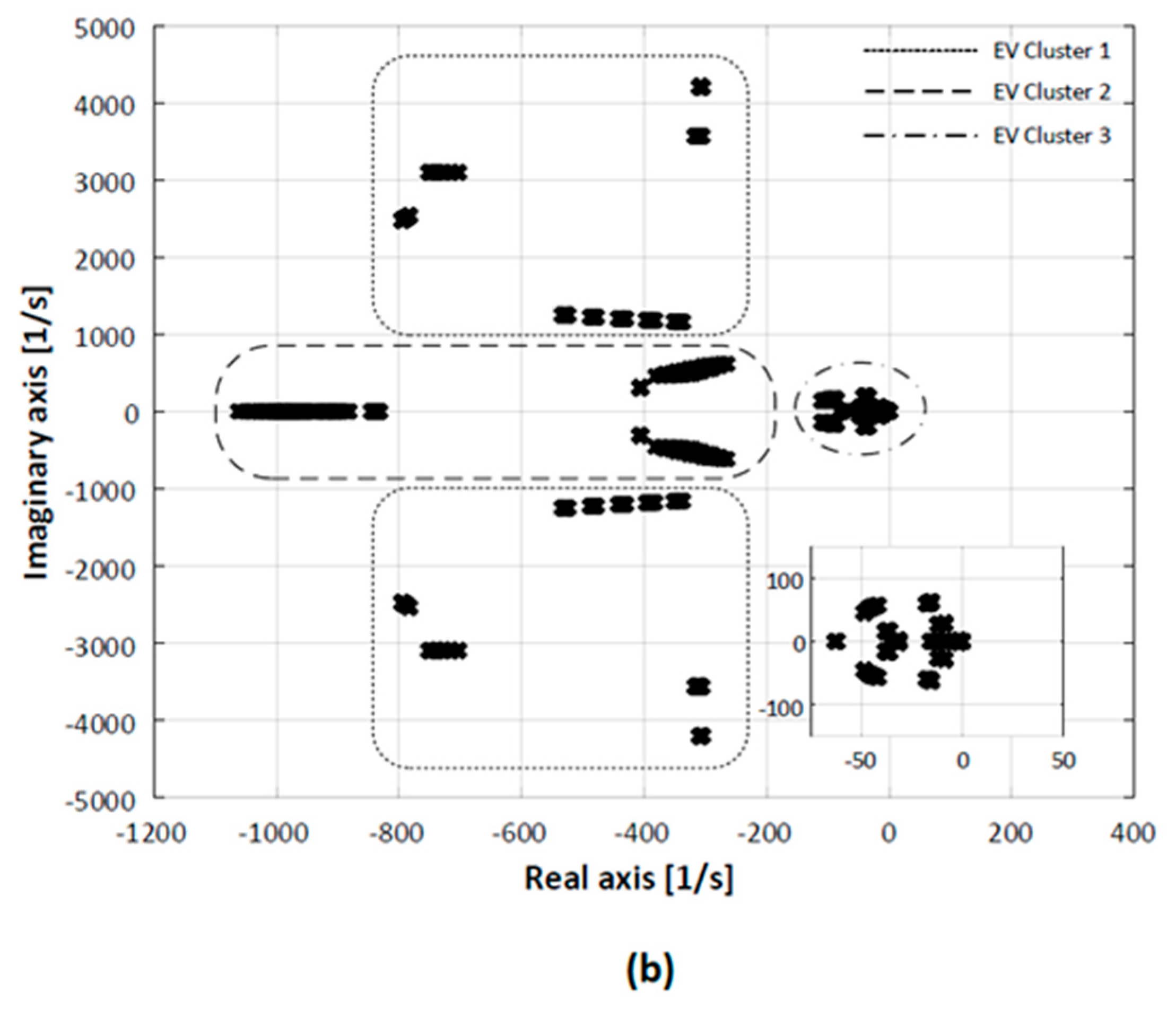
Figure 9a depicts the EV map for a scenario where all inverter based DERs and the genset are in operation. It can be seen that one EV pair is located in the right-half plane, indicating that the system is unstable. This EV has an eigenfrequency of $f_n\approx 18 \mathrm{Hz}$ and its damping ratio ranges between $\zeta =\left\{0.02,-0.1\right\}$.

In fact, negative damping is ascertained only during operating points where the BESS is in charging mode. This emphasizes the need for assessing the entire range of scenarios for HPP operation.

The PFs reveal that this oscillatory mode is associated with state variables of SG stator and rotor flux ($i_{gd}$, $i_{fd}$, $i_{kd}$) and of grid-forming inverter (${\phi }_{vcd}$, $i_{1d}$). In order to stabilize the system the focus needs to be laid on these particular state variables. On the one hand, it is not feasible to modify the physical characteristics of the genset. On the other hand, adjustments in the inverter control loops can result in a stable system. The cascaded control structure for voltage and current regulation is designed according to the physical characteristics of the inverter (i.e., LCL filter, switching frequency) [13]. Hence, re-tuning of these control loops might not be desired. Another way is to adjust the voltage feed-forward filter $G_{ff}\left(s\right)$ (see schematic diagram in Figure 4). The voltage feed-forward term is used to minimize the initial transient effect of the current. Generally, a filter with very high cut-off frequency (e.g., 20 kHz) is applied, and thus, it was neglected so far [28]. However, it can be adjusted to lower values to prevent system stability issues. Thereby, two additional state variables $v_{cd,avg}$ and $v_{cq,avg}$ are introduced to the state-space model (Equation (19)). The cut-off frequency is tuned to $f_{LPF,vc}=30 \mathrm{Hz}$ to yield a sufficient damping ratio of the EVs ($\zeta =0.42$).

$$\left[\begin{array}{c}\frac{d{v}_{cd,avg}}{dt}\\ \frac{d{v}_{cq,avg}}{dt}\end{array}\right]=2\pi \cdot f_{LPF,vc}\cdot \langle \left[\begin{array}{c}{v}_{cd}\\ v_{cq}\end{array}\right]-\left[\begin{array}{c}{v}_{cd,avg}\\ v_{cq,avg}\end{array}\right]\rangle$$

(19)

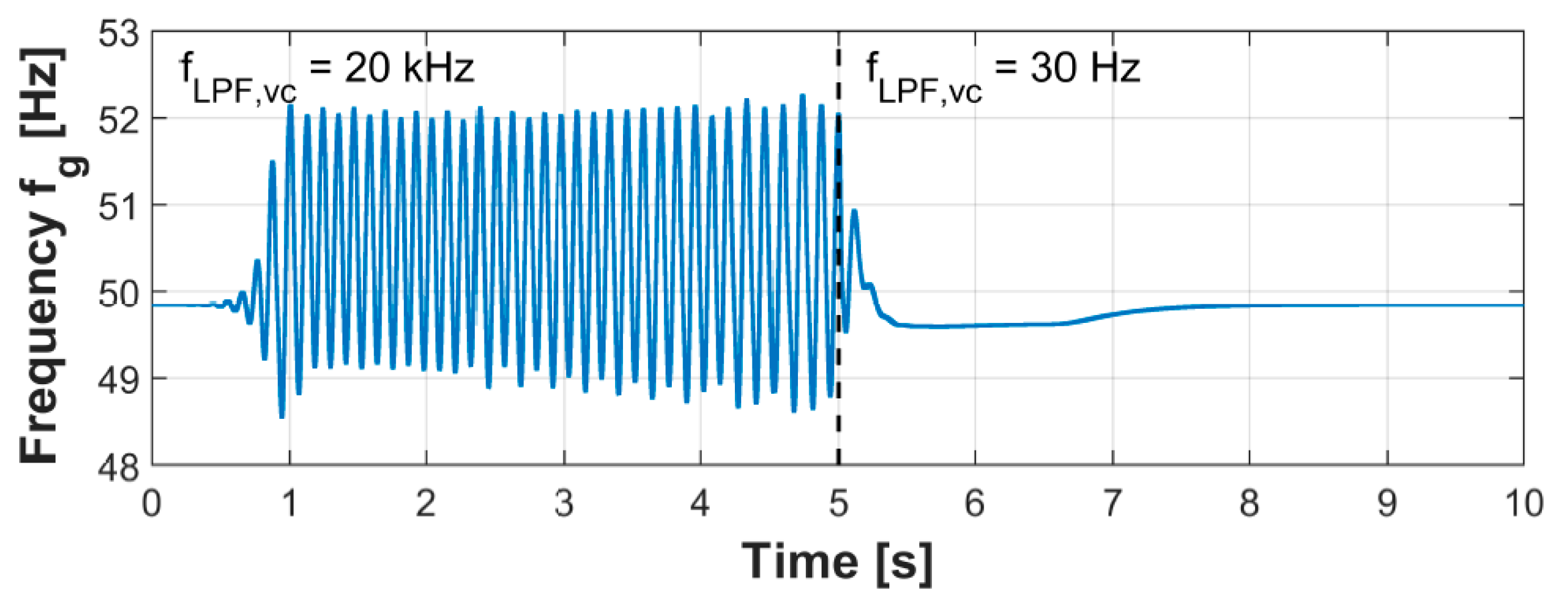
The EV map in Figure 9b demonstrates that the HPP is now stable in every operating condition. A time-domain simulation using a numerical model of the HPP (see Section 3.3) is performed to verify the observed stability phenomena. Figure 10 shows the grid frequency during a time interval $t=\left\{0,5\right\}s$ with $f_{LPF,vc}=20 \mathrm{kHz}$ and during a time range of $t=\left\{5,10\right\}\mathrm{s}$ where the filter cut-off frequency is adjusted to $f_{LPF,vc}=30 \mathrm{Hz}$. Grid frequency oscillations with negative damping are observed for $t<5 \mathrm{s}$, while the system stabilizes after filter tuning at $t=5 \mathrm{s}$.

In the next step, the occurring EVs, shown in Figure 9b, are characterized by means of

Table 2. Clustering of eigenvalues for test scenario 2 (stable case).

EV Cluster	Eigenfrequency ${\mathit{f}}_{\mathit{n}}$ [Hz]	Damping Ratio $\mathit{\zeta }$ [-]	Associated Dominant State Variables
1	{225, 20 × 103}	{0.03, 0.76}	Plant inductances and capacitances
2	{80, 160}	{0.61, 1}	Inverter inner current control loops, SG flux
3	{0.3, 34}	{0.19, 1}	Inverter outer control loops, SG flux, excitation system, genset mechanical time constants and control loops

. The resulting EV clusters are encircled in Figure 9.

The EVs in cluster #1 are associated with the same state variables as in test scenario 1.

The second cluster involves the dynamics of both inverters’ current controller and SG stator and rotor flux. All EVs in cluster #2 are sufficiently damped (ζ $\ge 0.61$).

The third EV group includes all dynamics within the frequency range of below 35 Hz. It is impossible to provide a more granular classification due to the vast number of state variables associated with each EV. The PF analysis revealed that the dynamic modes of cluster #3 are linked with inverters’ outer control loops and all genset dynamic states; i.e., electrical time constants of SG, mechanical time constants (inertia, prime mover) and control loops (governor, AVR). It should be noted that the presence of the genset introduces some dynamics in the very low frequency range ($f_n<2 \mathrm{Hz}$), caused by speed governor and AVR. In this test scenario, the critical EV ${\lambda }_{2,cr}$ with the lowest damping ratio ($\zeta =0.19$) exhibits an eigenfrequency of $f=11 \mathrm{Hz}$. The corresponding PFs indicate that state variables of grid-forming inverter ($P_{c,avg}$) and genset (${\omega }_r,{\delta }_r,P_{g,avg}$, $T_m$, ${\phi }_{G2}$) have a dominant impact on the EV. In conclusion, this dynamic mode is associated with the power sharing performance between grid-forming inverter and genset. Oscillatory behavior is caused by the inverter power measurement filter in combination with genset’s inertia and active power control.

The major conclusion from this subsection is that stability issues are of much more concern in scenario 2 (parallel operation of grid-forming inverter and genset) than in scenario 1 (operation with only inverter based DERs). Additionally, it is demonstrated by means of Figure 9 that the EVs of cluster #3 are located nearest to the imaginary axis. Hence, it is most crucial to observe the low frequency dynamics (<35 Hz) during the small-signal analysis.

4.4. Step IIId: Performing Sensitivity Analysis

A sensitivity analysis was applied to investigate the impact of various parameters on system stability during test scenario 2. Of particular interest is ${\lambda }_{2,cr}$, as it exhibits relatively low damping. The criterion for absolute system stability is $\zeta >0$. However, in order to avoid critically low damping of any voltage or frequency oscillations in the HPP, a reasonable target for the minimum damping ratio is ${\zeta }_{min}=0.05,$ as specified in Section 2.

4.4.1. Test Case 1: Power Measurement Filter of Grid-Forming Inverter

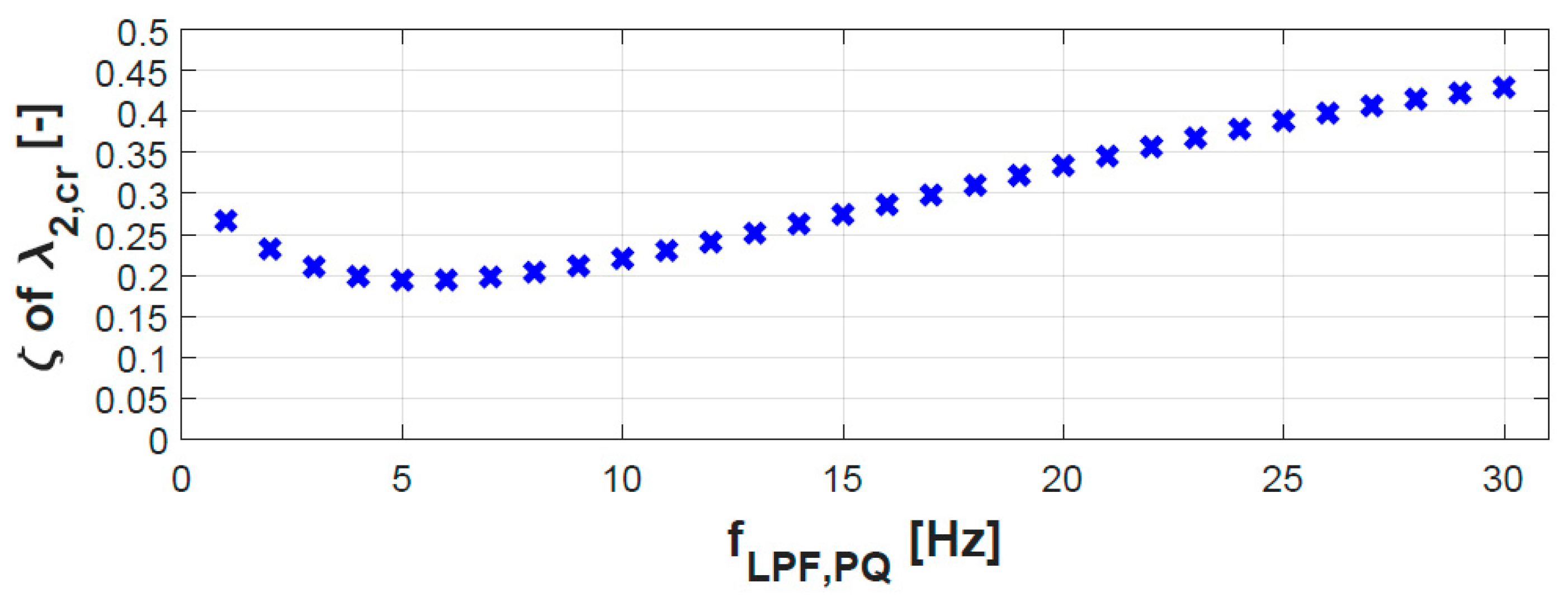
Power-based synchronization means that the grid-forming inverter is synchronized based on the power exchange between inverter and grid rather than measuring the voltage by means of PLL. The LPF of power measurements (see Figure 4) acts as a delay to any grid power variations, and hence affects the power sharing performance. Section 4.3 showed that the dynamic state of LPF ($P_{c,avg}$) is associated with ${\lambda }_{2,cr}$. Thus, the sensitivity of damping ratio to the filter cut-off frequency $f_{LPF,PQ}$ needs to be assessed. Up to now, a arbitrary value of $f_{LPF,PQ}=5\mathrm{Hz}$ has been applied. In Figure 11 the damping ratio of ${\lambda }_{2,cr}$ is shown for various values within $f_{LPF,PQ}=\left\{1,30\right\}\mathrm{Hz}$ and in steps of $\mathsf{\Delta }{f}_{LPF,PQ}=0.5 \mathrm{Hz}$. It is observed that the damping ratio $\zeta$ hits bottom at $f_{LPF,PQ}=5 \mathrm{Hz}$ and increases with rising values of $f_{LPF,PQ}$. However, it remains above $\zeta >0.15$. Thus, relative system stability is not seriously influenced by the value for $f_{LPF,PQ}$.

4.4.2. Test Case 2: Frequency/Active Power Droop Characteristic

The dynamic performance of power sharing between various DERs is dependent on the droop characteristic selected [13]. The correlation between frequency (or speed) and active power in steady-state is described by Equation (20), where $m_P$ is the so-called droop gain and ${\omega }^{*}$ and $P^{*}$ are frequency (or speed) reference and active power reference, respectively.

$$\omega -{\omega }^{*}=-m_P\cdot \left(P-P^{*}\right)$$

(20)

Typical values for the droop gain are in the range of $m_P=\left\{2,12\right\}\%$ [32]; however, an optimum range is yet to be ascertained.

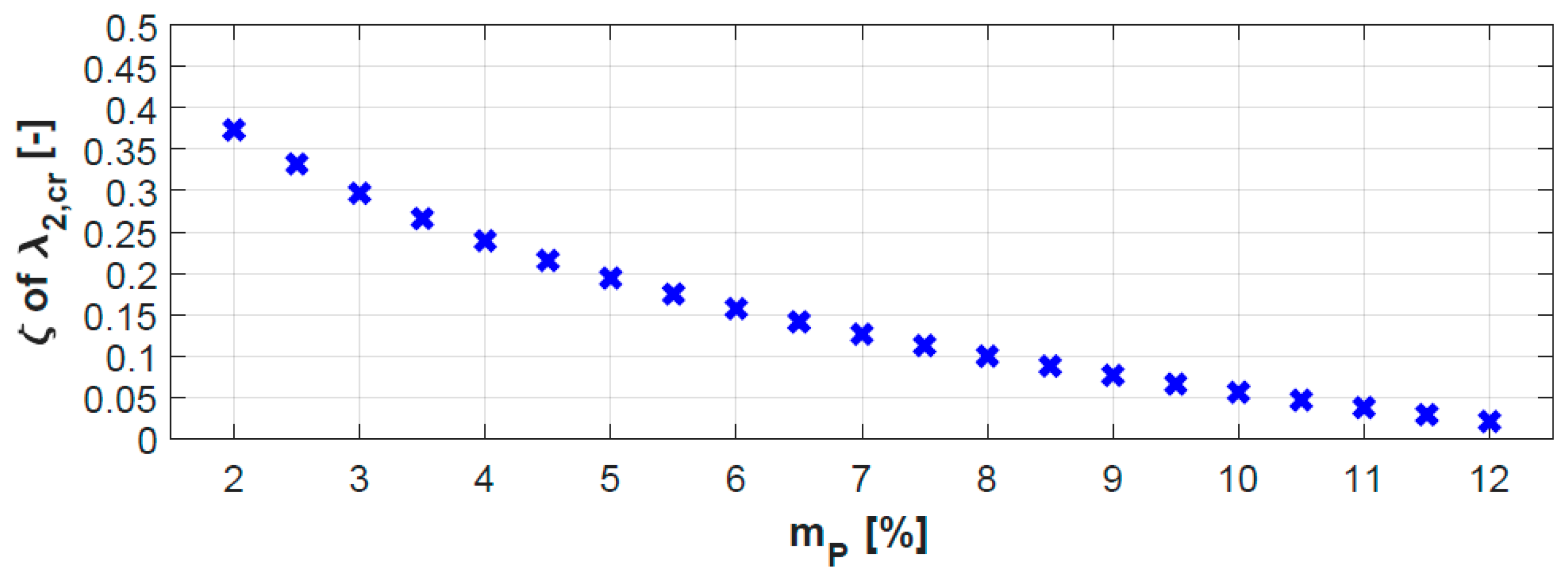
It is well known that the composite frequency/power characteristic of a power system contributes to the overall system damping [23]. In fact, there is an inverse relationship between system damping and droop gain $m_P$. Since EV ${\lambda }_{2,cr}$ is associated with state variables of both droop controlled DERs in the HPP, the sensitivity of its damping ratio to droop gain $m_P$ was investigated. The results are presented in Figure 12 where the droop gain was incremented with $\Delta m_P=1\%$. As expected, the damping ratio decreases significantly for increasing droop gains. It is not recommended to apply larger droop gains than $m_P>10\%$, as the damping ratio falls below the limit of ${\zeta }_{min}=0.05$.

The major conclusion from this section is that selecting feasible values for the droop gain $m_P$ are of much higher concern for system stability than tuning the power measurement filter of the grid-forming inverter due to large sensitivity of EV ${\lambda }_{2,cr}$ to droop gain $m_P$.

5. Step IV: Design and Tuning of Hybrid Power Plant Controller

This section deals with the design and subsequent tuning of the central HPPC. As explained in Section 2, primary control actions by DERs will leave steady-state errors in voltage and frequency which need to be compensated by secondary control actions of the central HPPC.

5.1. Step IVa: Designing Hybrid Power Plant Controller

Figure 13 depicts a system representation of the HPPC control architecture which is valid for both frequency and voltage control, yet being decoupled from each other. The plant system consists of DERs with primary voltage and frequency control (i.e., BESS and genset), the HPP internal grid consisting of the remaining DERs (i.e., WTG and PV), cables and transformers and a load which represents a disturbance to the system ($\mathsf{\Delta }{P}_{LD}$ and $\mathsf{\Delta }{Q}_{LD}$). The measurement block contains an LPF for voltage and frequency measurements, respectively. The time delay block $e^{-sT}$ reflects the communication ($T_{com}$) and sampling delay ($T_{s,HPPC}$) between HPPC and DERs when collecting all feedback signals and sending reference signals to the individual DERs. According to [33] an aggregated time delay describing the entire process can be defined by Equation (21).

$$T=0.5\cdot T_{s,HPPC}+T_{com}$$

(21)

The secondary control loop should be slower than the primary controller. Instead of a standard PI controller, a simple integral (I) controller with transfer function $G_{SC}\left(s\right)$ was chosen (Equation (22)), since control inputs and outputs have equal units, and thus, a proportional gain is not required.

$$G_{SC}\left(s\right)=\frac{1}{{\tau }_{SC}\cdot s}$$

(22)

The control time response ${\tau }_{SC}$ shall regard the minimum bandwidth of the plant system which can be described by means of transfer functions using the respective input and output signals ($u,y$) of the MIMO state-space model with ${\mathit{A}}_{\mathit{H}\mathit{P}\mathit{P}}$, ${\mathit{B}}_{\mathit{H}\mathit{P}\mathit{P}}$, ${\mathit{C}}_{\mathit{H}\mathit{P}\mathit{P}}$, ${\mathit{D}}_{\mathit{H}\mathit{P}\mathit{P}}$ and Equation (23) [23].

$$G_{u-y}\left(s\right)=\frac{\Delta y\left(s\right)}{\Delta u\left(s\right)}={\mathit{C}}_{\mathit{H}\mathit{P}\mathit{P}}{\left(s\mathit{I}-{\mathit{A}}_{\mathit{H}\mathit{P}\mathit{P}}\right)}^{-1}{\mathit{B}}_{\mathit{H}\mathit{P}\mathit{P}}+{\mathit{D}}_{\mathit{H}\mathit{P}\mathit{P}}$$

(23)

The secondary frequency controller was designed using $G_{{\omega }_{BESS}^{*}-{\omega }_g}$ and $G_{{\omega }_{GS}^{*}-{\omega }_g}$ The bandwidth of $G_{{\omega }_{BESS}^{*}-{\omega }_g}$ is infinite as the grid-forming inverter can regulate its frequency output almost instantenously. In case of the genset, the time response is given by speed governor and prime mover. Hence, the bandwidth ${\omega }_{bw}$ of $G_{{\omega }_{GS}^{*}-{\omega }_g}$ is applied to calculate the time response ${\tau }_{SC,f}$ of secondary frequency controller (Equation (24)).

$${\tau }_{SC,f}=\frac{1}{{\omega }_{bw}\left(G_{{\omega }_{GS}^{*}-{\omega }_g}\right)}$$

(24)

The secondary voltage controller is designed using $G_{V_{BESS}^{*}-V_{PCC}}$ and $G_{V_{GS}^{*}-V_{PCC}}$ The bandwidth of $G_{V_{BESS}^{*}-V_{PCC}}$ is around 20 times higher than of $G_{V_{GS}^{*}-V_{PCC}}$ due to relatively slow dynamics of AVR and excitation system. Hence, the bandwidth ${\omega }_{bw}$ of $G_{V_{GS}^{*}-V_{PCC}}$ is applied to calculate the time response ${\tau }_{SC,V}$ of secondary voltage controller (Equation (25)).

$${\tau }_{SC,f}=\frac{1}{{\omega }_{bw}\left(G_{V_{GS}^{*}-V_{PCC}}\right)}$$

(25)

The control sampling rate $T_{s,HPPC}$ is to be chosen according to the smallest time constant according to Nyquist (Equation (26)).

$$T_{s,HPPC}<0.5\cdot \min \left[\begin{array}{cc}{\tau }_{SC,f}& {\tau }_{SC,V}\end{array}\right]$$

(26)

5.2. Step IVb: Assessing Control Performance

In this subsection, the dynamic performance of the HPP voltage and frequency control is assessed by looking into step response characteristics in time-domain. This is accomplished by using the MIMO state-space model of the HPP. During the test cases it is assumed that no communication delays are present ($T_{com}=0$).

5.2.1. Test Case 1: Frequency Control

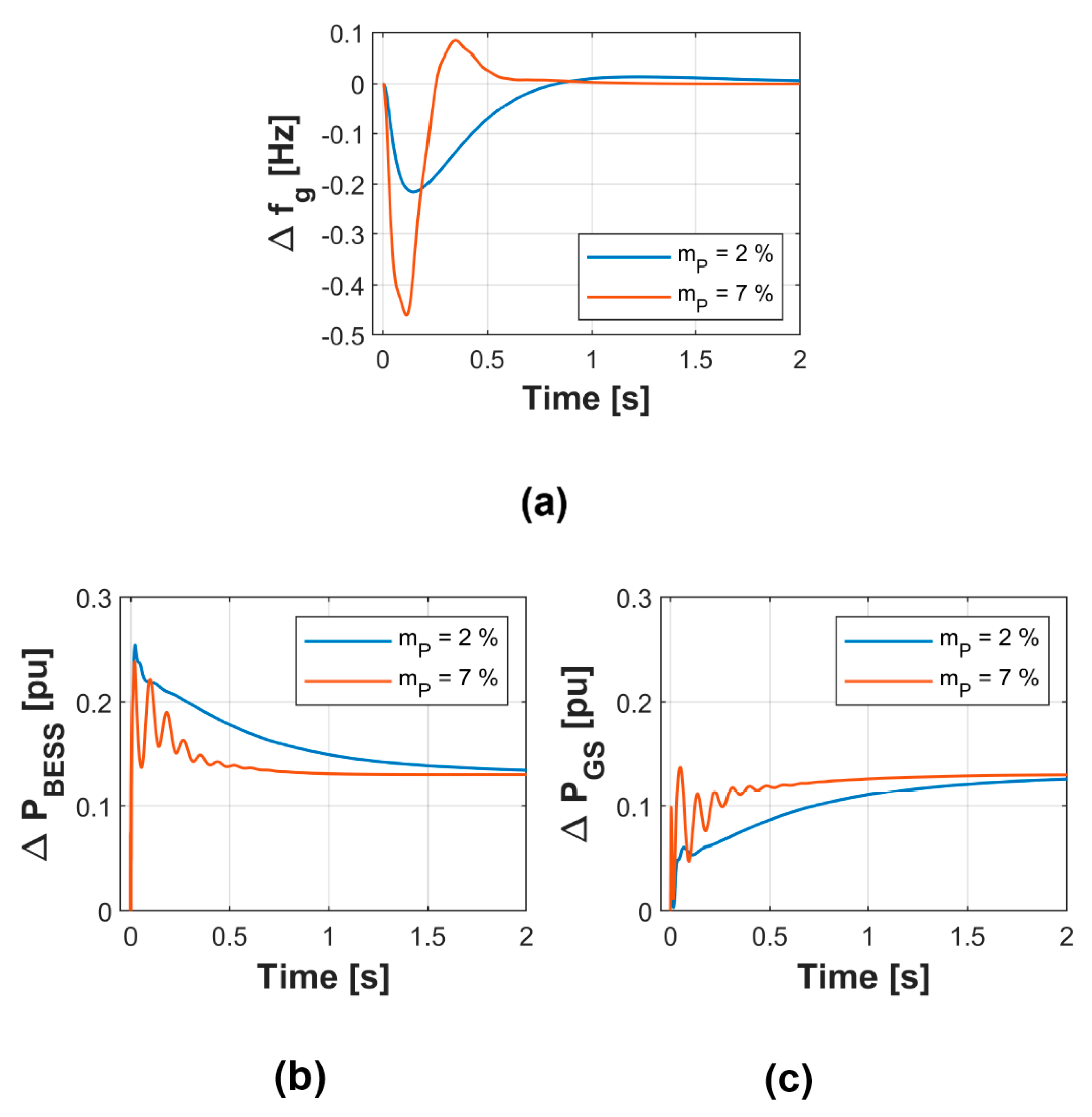
An active power load change of $\mathsf{\Delta }{P}_{LD}=0.25 \mathrm{pu}$ was applied as an input to the MIMO system of the HPP (see Figure 13) in order to test the performance of frequency regulation and active power sharing between grid-forming inverter and genset. In Figure 14 the output signals $\mathsf{\Delta }{f}_g$, $\mathsf{\Delta }{P}_{BESS}$ and $\mathsf{\Delta }{P}_{GS}$ of the MIMO system are shown for two different droop gains, $m_P=2\%$ and $m_P=7\%$, respectively.

As identified during the EV analysis (Section 4.2) the transient power oscillations are much more dominant for large droop gains due to decreased damping ratio of EV ${\lambda }_{2,cr}$. Larger values ($m_P>7\%$) lead to undesired low damping, and thus, were not further considered.

By observing the settling time of active power sharing, it can be concluded that small droop gains lead to prolonged transient response of $P_{BESS}$ and $P_{GS}$. While for $m_P=7\%$ the steady-state value was reached at $t=0.89 \mathrm{s}$, a new steady-state value is obtained at $t=2.45 \mathrm{s}$ for a droop gain of $m_P=2\%$.

The transient response of grid frequency $f_g$ is mainly affected with regard to its Nadir. A steep droop characteristic ($m_P=7\%$) leads to larger initial frequency deviations than a flat droop characteristic ($m_P=2\%$).

5.2.2. Test Case 2: Voltage Control

The aim of this test case is to assess the voltage control performance for various voltage/reactive power droop gains which typically lie within $m_Q=\left\{2,7\right\}\%$ [32]. The relation between voltage and reactive power is explained by Equation 27 where $V^{*}$ and $Q^{*}$ are voltage reference and reactive power reference, respectively.

$$V-V^{*}=-m_Q\cdot \left(Q-Q^{*}\right)$$

(27)

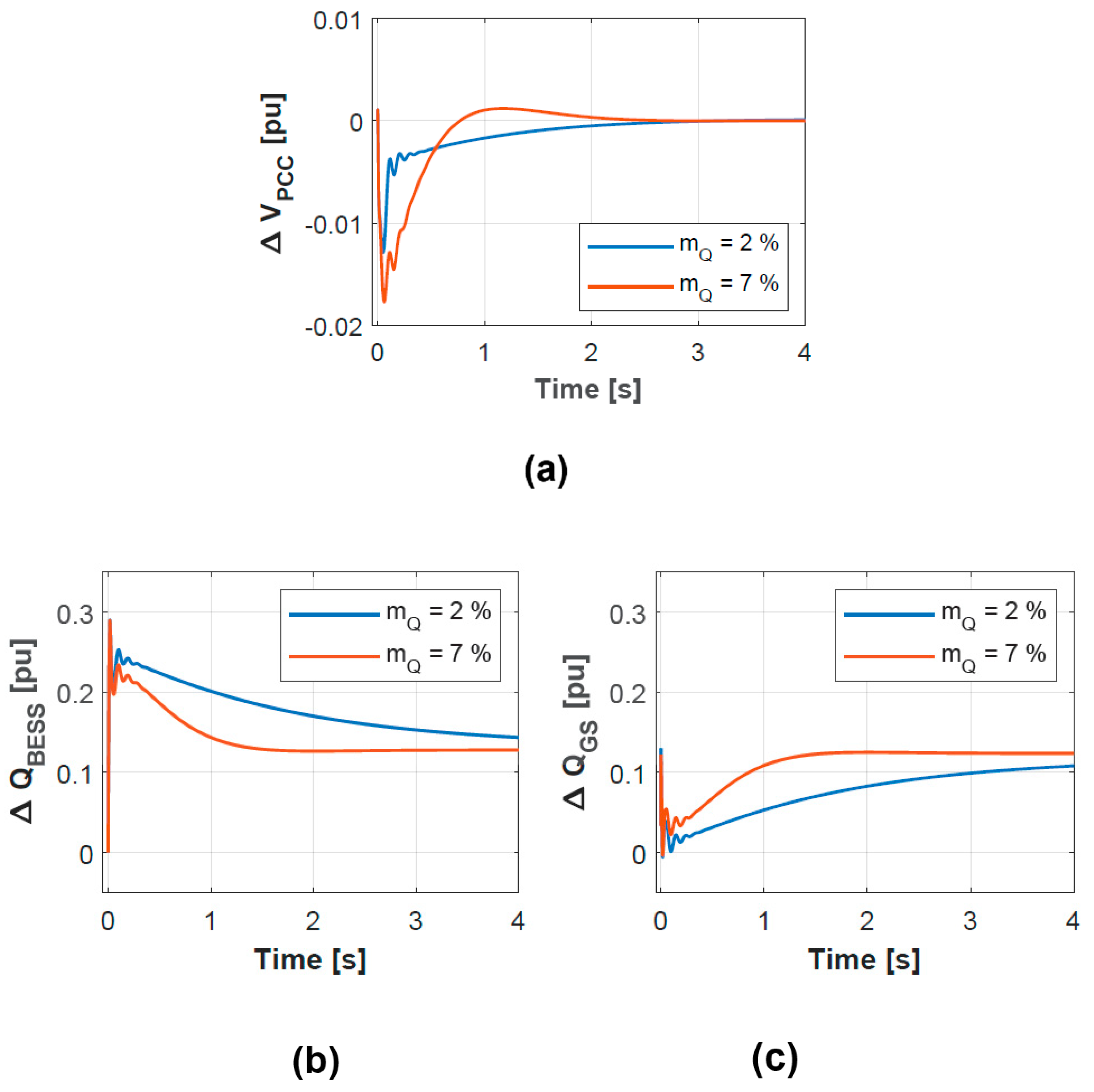
In order to assess the reactive power sharing performance between grid-forming inverter and genset, a reactive power load change of $\mathsf{\Delta }{Q}_{LD}=0.25 \mathrm{pu}$ was applied as an input to the MIMO system (see Figure 13). In Figure 15 the output signals $\mathsf{\Delta }{V}_{PCC}$, $\mathsf{\Delta }{Q}_{BESS}$ and $\mathsf{\Delta }{Q}_{GS}$ of the MIMO system are shown for the droop gains $m_Q=2\%$ (a) and $m_Q=7\%$ (b) respectively.

It was observed that the oscillatory behavior of voltage and reactive power was not affected by the droop gain.

With regard to settling time, similar conclusions to those in test case 1 were drawn: The steady-state value was reached at $t=1.40\mathrm{s}$ for a large droop gain $m_Q=7\%$, while for a small droop gain of $m_Q=2\%$ a new steady-state value was obtained much later at $t=6.55 \mathrm{s}$.

It is obvious from Figure 15 that the largest voltage drop occurs for a droop gain of $m_Q=7\%$. However, in both cases the remaining voltage drop is $\Delta V_{PCC}\gg -2\%$ for a reactive power load change of $\mathsf{\Delta }{Q}_{LD}=0.25 \mathrm{pu}$. Hence, it is not expected that the voltage limits are violated during a large-signal event (up to 100% change in reactive power) for any droop gain $m_Q$.

5.3. Step IVc: Control Tuning

The assessment studies have shown that the performance of voltage and frequency regulation is highly associated to the applied droop gains. In fact, the bandwidth values of the plant system, and hence the tuned parameters ${\tau }_{SC,f}$ and ${\tau }_{SC,V}$ of the secondary controller, depend on $m_P$ and $m_Q$, respectively. Several aspects are to be considered for selecting optimum droop gains:

• Frequency requirements: Figure 14 has shown that the frequency Nadir is deteriorated for large droop gains. Under-frequency load shedding (UFLS) schemes might be triggered depending on the occurring event (e.g., loss of unit) and UFLS characteristic. Detailed numerical simulations are required in order to assess such requirements.
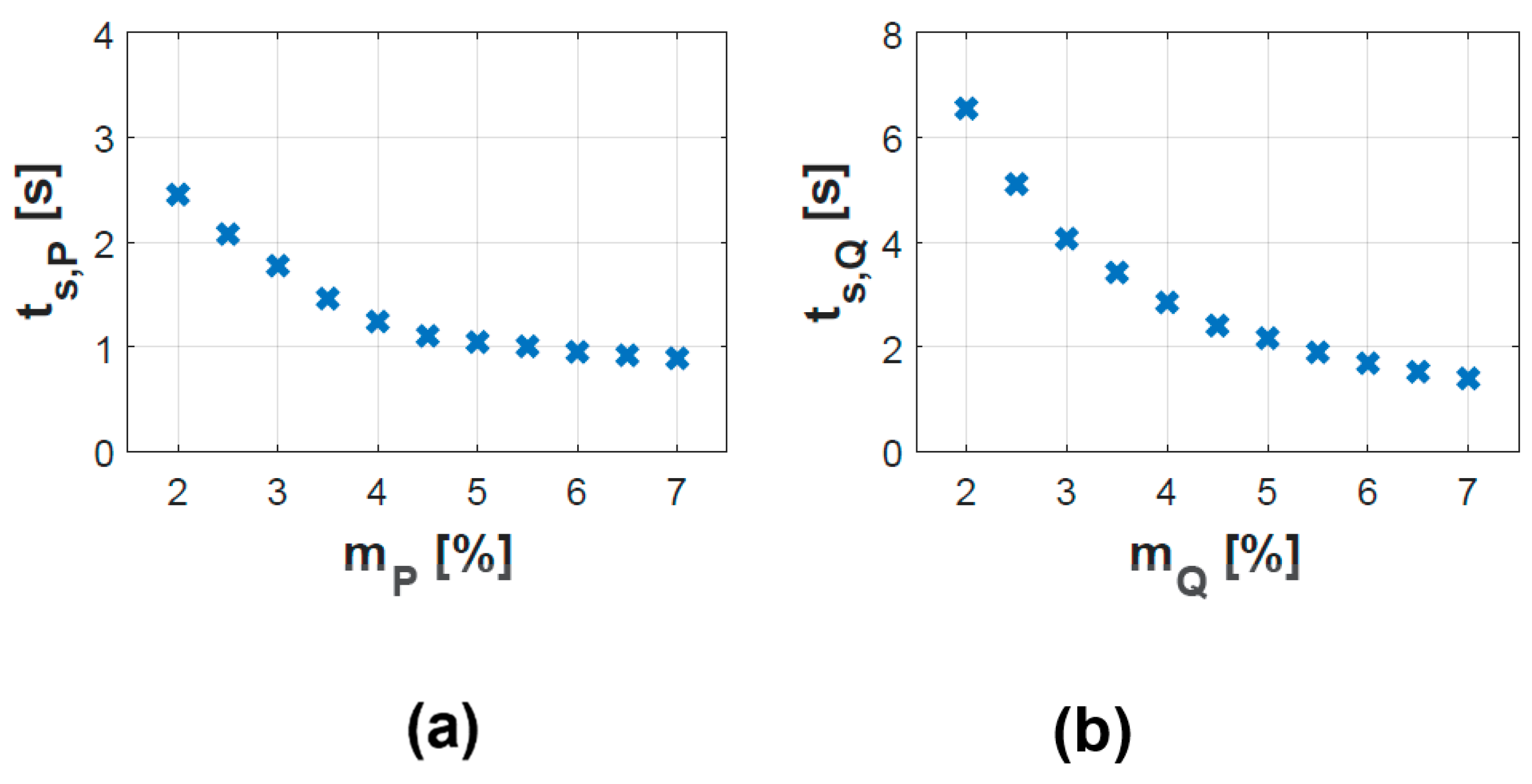
• Power sharing performance: Figure 16 summarizes in numbers how the settling time of active and reactive power increases with decreasing droop gains of BESS and genset. Proper droop gains shall be chosen according to the desired update rate of active and reactive power dispatch. Such a function is required, e.g., for BESS state-of-charge regulation and to avoid underloading/overloading of gensets according to dynamic fluctuations of renewable power. If active and reactive power setpoints are dispatched, e.g., every 3 s, the minimum droop gains shall be $m_P=2\%$ and $m_Q=4\%$ in order to allow settlement of the respective parameters (Figure 16).
• Control sampling rate: According to Equation (26) the required sampling rate $T_{s,HPPC}$ and hence the signal exchange between HPPC and DERs depends on the desired speed of secondary controller. In order to achieve the settling times depicted in Figure 16, the sampling rate must be $T_{s,HPPC}\le 50 \mathrm{ms}$ for $m_P=7\%$ and $T_{s,HPPC}\le 250 \mathrm{ms}$ for $m_P=2\%$. Hence, the computational power of the control platform and communication latency issues shall be well assessed prior to selecting a certain droop gain.

At this stage, it needs to be stressed that voltage and frequency control requirements for MGs/off-grid systems are usually not defined explicitly, and if so, are based on general technical guidelines only; e.g., as for rural electrification systems in [20]. However, the methodology for control design and tuning presented in this section enables to propose guidance on the practical implementation to the operators of such systems.

6. Step V: Rapid Control Prototyping

In this section, the performance of voltage and frequency control in the off-grid HPP shown in Figure 2 was evaluated by means of simulating representative test scenarios. While up to now all results were obtained by means of the linearized state-space model, in this section time-domain studies are described, which used discrete-time domain models (see Section 3.3) implemented in MATLAB SimPowerSytems Toolbox. In this way, the robustness of stability analysis and the HPPC design and tuning stage can be tested.

A set of wind speeds and solar irradiance measurements was utilized and fed into the performance models described in Section 3.3. A realistic aggregated load profile for the demand subsystem was applied where the load power factor was $\cos \phi =0.9$. The DER and HPPC settings during this test scenario are summarized in

Table 3. Test settings for rapid control prototyping.

	BESS	Genset	WTG	PV	HPPC
$P^{*}$ [kW]	$-45$	$45$	$80$	$40$	-
$Q^{*}$ [kW]	$0$	$0$	$20$	$10$	-
$m_P=m_Q$ [%]	$5$	$5$	-	-	-
$T_{s,HPPC}$ [ms]	-	-	-	-	$50$

.

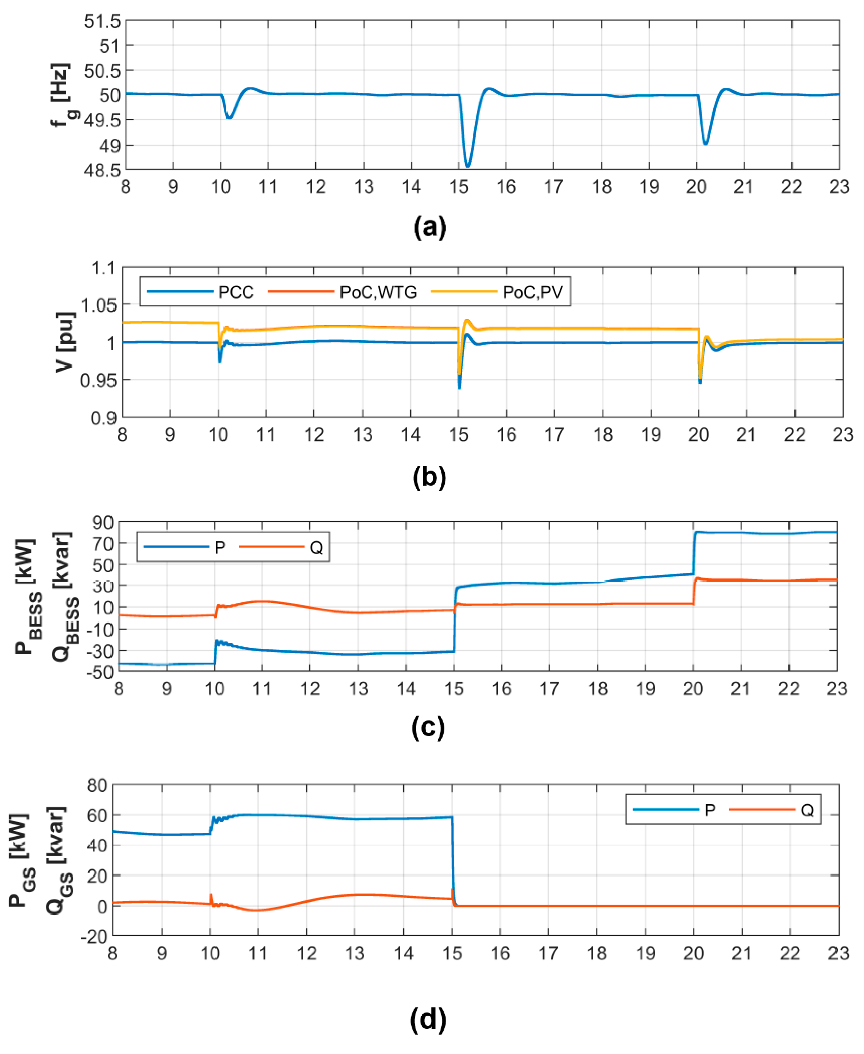
The following events are simulated in order to assess voltage and frequency control during various operating modes:

0.

Operation with all DERs until $t<10 s$;

1.

Disconnection of PV at $t=10 s$;

2.

Disconnection of genset at $t=15 s$;

3.

Disconnection of WTG at $t=20 s$.

Figure 17 presents the resulting grid frequency (a), voltage (b) and active and reactive power profiles (Figure 17c–g). The results show that grid frequency and PCC voltage are regulated to 1 pu after every single event. Power is shared evenly between BESS and genset after PV disconnection. The largest drop of frequency and voltage occurs after genset tripping, since it is highly loaded ($P_{GS}\left(t=14.9 \mathrm{s}\right)\approx 60 \mathrm{kW}$) and the BESS needs to solely compensate for the power deficit.

Usually, during the RCP stage iterations of control design and tuning are expected depending on the performed tests and their outcome. However, the presented simulation studies demonstrate the effectiveness of performing stability analysis and control design/tuning for voltage and frequency control by applying linearized state-space models which have been validated against numerical models. In this way, the entire MBD process is accelerated.

7. Step VI and VII: Control Verification and Validation

7.1. Step VI: Real-Time Hardware-in-the-Loop Verification

As a final step of MBD in HPPs, the control algorithms were implemented on a controller platform and tested. Verification of the HPPC was accomplished by connecting the controller platform to a RT model of the power system including DERs; i.e., WTGs, PV system, BESS, gensets. Moreover, for realistic testing a RT model of the communication networks was used. Thus, the controller platform including the developed algorithms could be assessed in realistic conditions. Grid events that cannot be measured in real life can also be replicated in a controlled environment while data traffic associated to specific communication network technologies are captured properly without actually involving the real technologies [34].

One might argue the verification stage might be dropped and on-site testing of off-grid HPPs can be realized immediately as being independent of any external grid parameters. However, it seems impracticable and cumbersome to deploy and test HPPCs on-site for remote applications, before gaining further confidence by extensive testing and verification in a controlled system environment.

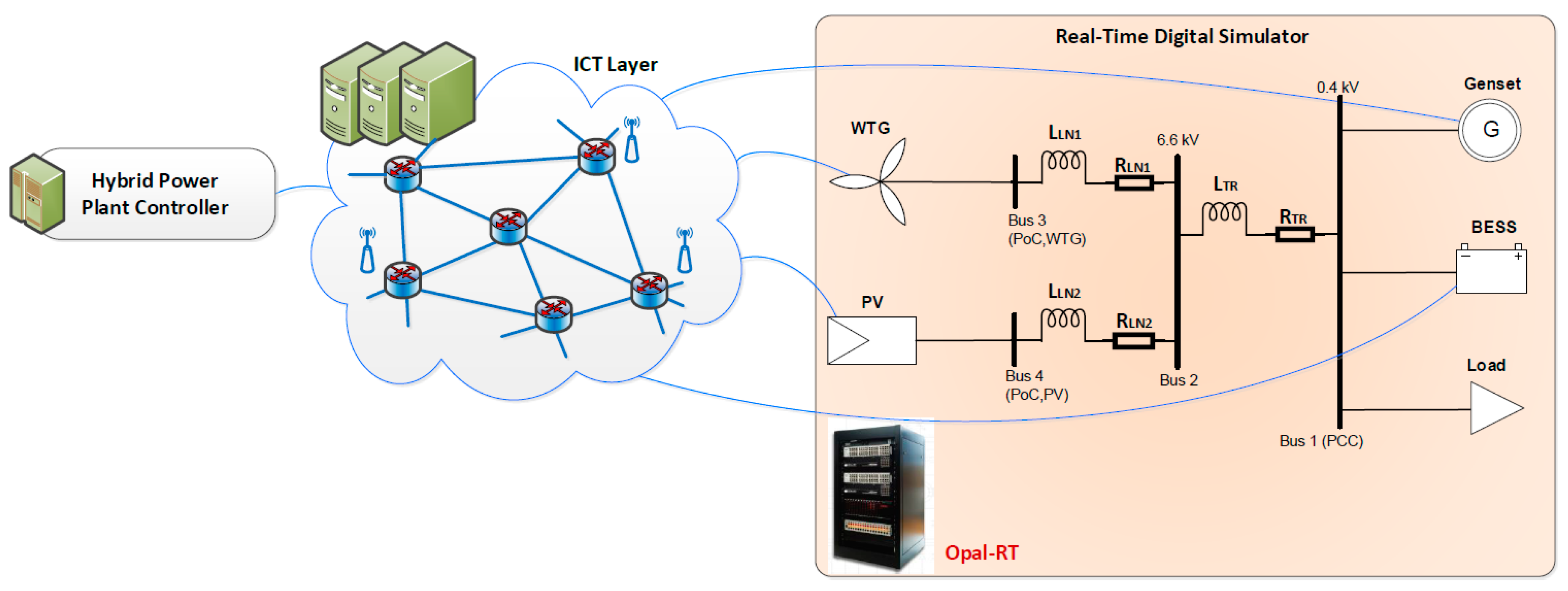
The existing facilities in the Smart Energy Systems Laboratory at Aalborg University allowed all the above design and verification procedure. The architecture of this platform is shown in Figure 18 [35]. The information and communication technology (ICT) layer is the backbone for the setup and aims to emulate different technologies and topologies for the communication network. It is crucial to account for communication bandwidth, latency and potential packet losses for all signals being exchanged between HPPC and DERs. The RT digital simulator was based on OPAL-RT technology. Here, the numerical DER models developed in MATLAB SimPowerSystems and utilized during RCP stage can be re-used with minor adjustments. OPAL-RT’s automatic code generation process enables one to easily compile models. The HPPC platform is based on Bachmann PLC technology. Here, a similar process allows the use of control algorithms in MATLAB Simulink and subsequent deployment of controller models to the PLC without manual coding.

7.2. Step VII: On-Site Testing

The actual controller platform was tested on-site under operating conditions allowed by the physical power grid and assets. The testing campaign is typically limited in time and power system events in scope for the developed algorithms; e.g., large voltage and frequency excursions might not occur in the system during this period. Thus, an open loop approach is used. This means that the controller is fed with pseudo-measurements and the output of the plants is recorded. However, the actual impact on the power grid cannot be evaluated, nor can possible control interactions between assets. These recordings might be used to validate the numerical models developed and used in the previous stages. In fact, the performance models of WTG, PV and BESS applied during the RCP stage (Section 6) have been validated by field data and are presented in another publication [31].

8. Conclusions and Outlook

This paper proposes a detailed and practical guidance on applying MBD for voltage/frequency stability analysis, control tuning and verification in off-grid HPPs comprising both grid-forming and grid-feeding inverter units and synchronous generation. The different stages are summarized by means of Figure 1.

Initially, system and functional requirements for voltage and frequency regulation and the modeling requirements for assessment studies are specified in Section 2.

Then, a modular approach of setting up the state-space model is described by means of a benchmark HPP system used in this study (Section 3). Flexible merging of subsystems by properly defining input and output vectors is highlighted to describe the dynamics of the HPP during various operating states. The state-space models were used during the stability assessment and control tuning stage. Numerical simulation models were prepared in parallel based on the work in [31] and are applicable for small-signal model validation and the control verification stage.

EV and PF analyses were performed as part of the stability assessment (Section 4). The studies reveal that during particular load conditions instable dynamic modes occur which can be stabilized by tuning the inverter feed-forward filter. Furthermore, it is shown that clustering the vast number of system EVs enables one to identify critical dynamic modes with low damping ratio. A sensitivity analysis addresses the impact of relevant system parameters on these critical EVs. It is ascertained that false parametrization of active power/frequency characteristic by selecting large droop gains will move the system towards instability.

Subsequently, the control loops of the central HPP controller are designed with the purpose of frequency and voltage restoration (Section 5). It was demonstrated that the control performance largely depends on the applied droop gains of voltage and frequency regulating DERs. Some suggestions are provided for control tuning according to requirement specifications.

The RCP stage is accomplished by means of discrete-time domain models (Section 6). The off-line simulation studies confirm the effectiveness of performing stability analysis and control design/tuning for voltage and frequency control in the off-grid HPP.

An outlook is given for verifying the HPPC platform by means of RT-HIL testing as the final step of proof-of-concept (Section 7). The control algorithms developed, including physical implementation on target hardware, are then ready for site testing.

Overall, the proposed MBD approach fulfills the specified requirement specifications. It involves thorough stability assessment and control tuning stages which reduce iterations between various MBD stages significantly. The modeling effort is minimized by the use of validated discrete-time domain models of DERs in both RCP and control verification stages. Extensive RT-HIL testing in the described test setup [34] yields in high level of confidence where the need for control validation (step VII) can be significantly reduced.

The outcome of this paper is targeted at off-grid HPP operators seeking to achieve a proof-of-concept on stable voltage and frequency regulation. Nonetheless, the overall methodology is applicable to utility scale HPPs as well, where design and tuning criteria are given by the respective grid codes.

References

- Elkadragy, M.M.; Baumann, M.; Moore, N.; Weil, M.; Lemmertz, N. Contrastive Techno-Economic Analysis Concept for Off-Grid Hybrid Renewable Electricity Systems Based on comparative case studies within Canada and Uganda. In Proceedings of the 3rd International Hybrid Power Systems Workshop, Tenerife, Spain, 8–9 May 2018; Energynautics: Darmstadt, Germany. [Google Scholar]
- Bitaraf, H.; Buchholz, B. Reducing energy costs and environmental impacts of off-grid mines. In Proceedings of the 3rd International Hybrid Power Systems Workshop, Tenerife, Spain, 8–9 May 2018; Energynautics: Darmstadt, Germany. [Google Scholar]
- Petersen, L.; Iov, F.; Tarnowski, G.C.; Carrejo, C. Optimal and Modular Configuration of Wind Integrated Hybrid Power Plants for Off-Grid Systems. In Proceedings of the 3rd International Hybrid Power Systems Workshop, Tenerife, Spain, 8–9 May 2018; Energynautics: Darmstadt, Germany. [Google Scholar]
- Kumar, R.; Gupta, R.A.; Bansal, A.K. Economic analysis and power management of a stand-alone wind/photovoltaic hybrid energy system using biogeography based optimization algorithm. Swarm Evol. Comput. 2013, 8, 33–43. [Google Scholar] [CrossRef]
- Maitra, A.; Rogers, L.; Handa, R. Program on Technology Innovation: Microgrid Implementations: Literature Review, Report; Electric Power Research Institute: Palo Alto, CA, USA, 2016; Available online: epri.com (accessed on 30 November 2019).
- Hafez, O.; Bhattacharya, K. Optimal planning and design of a renewable energy based supply system for microgrids. Renew. Energy 2012, 45, 7–15. [Google Scholar] [CrossRef]
- Ghiani, E.; Vertuccio, C.; Pilo, F. Optimal sizing of multi-generation set for off-grid rural electrification. In Proceedings of the IEEE Power and Energy Society General Meeting, Boston, MA, USA, 17–21 July 2016; IEEE: Piscataway, NJ, USA, 2016; pp. 1–5. [Google Scholar]
- Cañizares, C.A. Microgrid Stability Definitions, Analysis and Modeling; IEEE Power & Energy Society: Piscataway, NJ, USA, 2018. [Google Scholar]
- Pogaku, N.; Member, S.; Prodanovic, M.; Green, T.C.; Member, S. Modeling, Analysis and Testing of Autonomous Operation of an Inverter-Based Microgrid. IEEE Trans. Power Electron. 2007, 22, 613–625. [Google Scholar] [CrossRef] [Green Version]
- Etemadi, A.H.; Iravani, R. Eigenvalue and Robustness Analysis of a Decentralized Voltage Control Scheme for an Islanded Multi-DER Microgrid. In Proceedings of the IEEE Power and Energy Society General Meeting, San Diego, CA, USA, 22–26 July 2012; IEEE: Piscataway, NJ, USA, 2012. [Google Scholar]
- Tang, X.; Deng, W.; Qi, Z. Investigation of the dynamic stability of microgrid. IEEE Trans. Power Syst. 2014, 29, 698–706. [Google Scholar] [CrossRef]
- Katiraei, F.; Iravani, M.R.; Lehn, P.W. Small-signal dynamic model of a micro-grid including conventional and electronically interfaced distributed resources. IET Gener. Transm. Distrib. 2007, 1, 324. [Google Scholar] [CrossRef] [Green Version]
- Gkountaras, A. Modeling Techniques and Control Strategies for Inverter Dominated Microgrids. Ph.D. Thesis, Technical University of Berlin, Berlin, Germany, 2017. Available online: depositonce.tu-berlin.de (accessed on 30 November 2019).
- Rocabert, J.; Luna, A.; Blaabjerg, F. Control of Power Converters in AC Microgrids. IEEE Trans. Power Electron. 2012, 27, 4734–4749. [Google Scholar] [CrossRef]
- Guerrero, J.M.; Vasquez, J.C.; Matas, J.; De Vicuna, L.G.; Castilla, M. Hierarchical Control of Droop-Controlled AC and DC Microgrids—A General Approach Toward Standardization. IEEE Trans. Ind. Electron. 2011, 58, 158–172. [Google Scholar] [CrossRef]
- Guerrero, J.M.; Matas, J.; Garcia de Vicuna, L.; Castilla, M.; Miret, J. Decentralized Control for Parallel Operation of Distributed Generation Inverters Using Resistive Output Impedance. IEEE Trans. Ind. Electron. 2007, 54, 994–1004. [Google Scholar] [CrossRef]
- Hadisupadmo, S.; Hadiputro, A.N.; Widyotriatmo, A. A Small Signal State Space Model of Inverter-Based Microgrid Control on Single Phase AC Power Network. Internetworking Indones. J. 2016, 8, 71–76. [Google Scholar]
- Petersen, L.; Iov, F.; Tarnowski, G.C.; Raghuchandra, K.B. Methodological Framework for Stability Analysis, Control Design and Verification in Hybrid Power Plants. In Proceedings of the 4th International Hybrid Power Systems Workshop, Crete, Greece, 22–23 May 2019; Energynautics: Darmstadt, Germany, 2019. [Google Scholar]
- EirGrid. Operating Security Standards; EirGrid: Dublin, Ireland, 2011. [Google Scholar]
- IEC 62257. Recommendations for Renewable Energy and Hybrid Systems for Rural Electrification—Part 2: From Requirements to a Range of Electrification Systems; International Electrotechnical Commission: Geneva, Switzerland, 2016. [Google Scholar]
- IEEE Standards Department. P2030.7/D11 Draft Standard for Specification of Microgrid Controllers; IEEE: Piscataway, NJ, USA, 2017. [Google Scholar]
- Steinhart, C.J.; Finkel, M.; Gratza, M.; Witzmann, R.; Kerber, G.; Verteilnetz, L.E.W.; Germany, G. Determination of Load Frequency Dependence in Island Power Supply. In Proceedings of the 24th International Conference on Electricity Distribution, Glasgow, UK, 12–15 June 2017; pp. 12–15. [Google Scholar]
- Kundur, P. Power System Stability and Control; McGraw-Hill, Inc.: New York, NY, USA, 1993. [Google Scholar]
- Petersen, L.; Kryezi, F.; Iov, F. Design and tuning of wind power plant voltage controller with embedded application of wind turbines and STATCOMs. IET Renew. Power Gener. 2017, 11, 216–225. [Google Scholar] [CrossRef] [Green Version]
- Huang, H.; Mao, C.; Lu, J.; Wang, D. Small-signal modelling and analysis of wind turbine with direct drive permanent magnet synchronous generator connected to power grid. IET Renew. Power Gener. 2012, 6, 48–58. [Google Scholar] [CrossRef]
- Anderson, P.M.; Fouad, A.A. Power System Control and Stability; Wiley-IEEE Press: Hoboken, NJ, USA, 1995; ISBN 007035958X. [Google Scholar]
- Knudsen, J. Modeling, Control and Optimization for Diesel-Driven Generator Sets. Ph.D. Thesis, Aalborg University, Aalborg, Denmark, 2017. Available online: vbn.aau.dk (accessed on 30 November 2019).
- Yazdani, A.; Iravani, R. Voltage-Sourced Converters in Power Systems: Modeling, Control and Applications; IEEE Press: Piscataway, NJ, USA; John Wiley: Hoboken, NJ, USA, 2010; ISBN 9780470521564. [Google Scholar]
- Teodorescu, R.; Liserre, M.; Rodríguez, P. Grid Converters for Photovoltaic and Wind Power Systems; John Wiley & Sons, Ltd.: Hoboken, NJ, USA, 2010; ISBN 9780470057513. [Google Scholar]
- Sabor, O. Small-Signal Modelling and Stability Analysis of a Traditional Generation Unit and a Virtual Synchronous Machine in Grid-Connected Operation. Master’s Thesis, Norwegian University of Science and Technology, Trondheim, Norway, 2015. Available online: repository.tudelft.nl (accessed on 30 November 2019).
- Petersen, L.; Iov, F.; Tarnowski, G.C.; Gevorgian, V.; Koralewicz, P.; Stroe, D.-I. Validating Performance Models for Hybrid Power Plant Control Assessment. Energies 2019, 12, 4330. [Google Scholar] [CrossRef] [Green Version]
- European Commission. Network Code on Requirements for Grid Connection of Generators; European Network of Transmission System Operators for Electricity: Brussels, Belgium, 2016. [Google Scholar]
- Garcia, J.M. Voltage Control in Wind Power Plants with Doubly Fed Generators. Ph.D. Thesis, Aalborg University, Aalborg, Denmark, 2010. Available online: vbn.aau.dk (accessed on 30 November 2019).
- Iov, F.; Shahid, K.; Petersen, L.; Olsen, L.R. RePlan Project: D5.1—Verification of Ancillary Services in Large Scale Power System, Project Report, Aalborg, Denmark. 2018. Available online: www.replanproject.dk (accessed on 30 November 2019).
- Smart Energy Systems Laboratory at Aalborg University. Available online: www.et.aau.dk/laboratories/power-systems-laboratories/smart-energy-systems (accessed on 30 November 2019).
Figure 1.
Proposed model-based design (MBD) approach for stability assessment, control tuning and verification in off-grid hybrid power plants (HPPs).
Figure 2.
Single-line diagram of off-grid HPP (black) and functional diagram of state-space model (red).
Figure 3.
Relationship of voltage space vector components in local reference (qd) and global (DQ) reference frame (a) for inverter based units and (b) for genset.
Figure 4.
Schematic diagram of grid-forming inverter.
Figure 5.
Schematic diagram of grid-feeding inverter.
Figure 6.
Schematic diagram of generator set.
Figure 7.
Schematic diagram of numerical models applicable to rapid control prototyping (RCP) and control verification: (a) wind turbine generator (WTG); (b) photovoltaic (PV).
Figure 8.
Eigenvalue map of AHPP—Test scenario 1: only inverter based distributed energy resources (DERs) in operation.
Figure 9.
Eigenvalue maps of AHPP—Test scenario 2: all DERs in operation: (a) unstable case; (b) stable case.
Figure 10.
Verification of stability phenomena by time-domain simulations.
Figure 11.
Sensitivity of damping ratio of critical eigenvalues (EV) to low pass filter (LPF) cut-off frequency .
Figure 12.
Sensitivity of damping ratio of critical EV to f/P droop gain .
Figure 13.
System representation for hybrid power plant voltage and frequency controller.
Figure 14.
Transient load sharing performance between abattery energy storage system (BESS) and fossil fuel generator set (genset) for various f/P droop gains ; (a) frequency; (b) BESS active power; (c) genset active power.
Figure 15.
Transient load sharing performance between BESS and genset for various V/Q droop gains (a) PCC voltage; (b) BESS reactive power; (c) genset reactive power.
Figure 16.
Settling time of (a) active power () and (b) reactive power () of BESS and genset for various droop gains and .
Figure 17.
Results of control verification using discrete-time domain simulation models.
Figure 18.
RT-HIL Co-Simulation Architecture in Smart Energy Systems Laboratory [35].