Structural Condition for Controllable Power Flow System Containing Controllable and Fluctuating Power Devices


Graduate School of Advanced Science and Technology, Japan Advanced Institute of Science and Technology, 1-1 Asahidai, Nomi City 923-1296, Japan
*
Author to whom correspondence should be addressed.
Energies 2020, 13(7), 1627; https://0-doi-org.brum.beds.ac.uk/10.3390/en13071627
Submission received: 5 March 2020
/
Revised: 19 March 2020
/
Accepted: 20 March 2020
/
Published: 2 April 2020
(This article belongs to the Special Issue Microgrids: Planning, Protection and Control)
Abstract
:This paper discusses a structural property for a power system to continue a safe operation under power fluctuation caused by fluctuating power sources and loads. Concerns over global climate change and gas emissions have motivated development and integration of renewable energy sources such as wind and solar to fulfill power demand. The energy generated from these sources exhibits fluctuations and uncertainty which is uncontrollable. In addition, the power fluctuations caused by power loads also have the same consequences on power system. To mitigate the effects of uncontrollable power fluctuations, a power flow control is presented which allocates power levels for controllable power sources and loads and connections between power devices. One basic function for the power flow control is to balance the generated power with the power demand. However, due to the structural limitations, i.e., the power level limitations of controllable sources and loads and the limitation of power flow channels, the power balance may not be achieved. This paper proposes two theorems about the structural conditions for a power system to have a feasible solution which achieves the power balance between power sources and power loads. The discussions in this paper will provide a solid theoretical background for designing a power flow system which proves robustness against fluctuations caused by fluctuating power devices.
1. Introduction
The awareness of depletion of fossil fuels, increase of power demand, and global warming have promoted the development of renewable energy sources. These energy sources such as wind turbines and photovoltaic (PV) generation system play important roles because of low impact against the environment. However, the generated power from these energy sources varies greatly, resulting in a risk of power fluctuations which is uncontrollable [1]. Renewable energy sources are often connected to the medium-and-low-voltage grid in smaller unit sizes. With the rapid increase of renewable energy sources, the increase of power fluctuation in the power system gives cause for anxiety [2]. The power fluctuations phenomenon caused by power loads also have the same consequences. The power demand is continuously growing due to the development of the smart consumer electronics equipped with communication and control units [3,4,5]. Moreover, the introduction of heat pumps and the electric cars are also contributing to a higher power demand. The mixture of renewable energy generation attached to grid and ever-growing power demand have increased the threats of stability and quality of power of the national wide power grid. As a result, the power system needs new strategies for the management and operation of the electricity to maintain balance between changing power supply patterns and consumption patterns [6].
Recently, the interest in the demand side management has been increased [7,8,9,10,11]. This is particularly because residential and commercial domains represent a major part of electricity consumption and carbon gas emissions [12] and partly because small scale distributed power resources such as photovoltaic, wind turbines, fuel cells, and storage batteries are introducing into houses, buildings, offices, and factories etc. The power structure of these facilities is changing dynamically due to the integration of distributed power sources [13,14]. One example of such changing structure is a Nano-grid (NG) [15,16,17]. It includes numerous power generating sources, an in-house or building power distribution system, and energy storage functions as well as a variety of consumer devices such as lighting, TV, heating/ventilation/air-conditioning, and cooking, i.e., such power systems need to have a sophisticated power control function that can manage dynamically changing power consumption and power supply conditions. We believe this is a new power control function to be developed for these changing power structures.
Due to the uncontrollability of generated power and demand, the power imbalance is a big challenge to consider [18,19]. In the fluctuating environment where power supply and demand both change dynamically and uncontrollably, a real-time power flow control is required, whose main function is to keep the balance between generated power and demand. There have been proposed several implementation models that can be classified into power switching and power packetization. Okabe et al. in [20] proposed a power switch between a multiple power sources and loads. The proposed system architecture for power switching is comprise of power sources, loads, power switch/router and power transmission lines. A physical power line connection is created between a power source and a load. The power control introduced is very simple and support only one-to-one and one-to-many connections types between power sources and loads. However, the power control cannot be enhanced when number of devices increased without changing the existing grid structure to manage many to one connection type. The power fluctuation management and control is out of the scope for this method. Abe et al. [21] and Hikihara et al. [22] proposed power packetization methods. The system design consists of group of power sources, loads, storage battery, power routers, and power lines. They introduced power routers which are able to receive, store, and transmit power, in power packets, a power packet is associated with source ID and destination ID. This method also implements a simple power control; however, explicit power control for uncertainty due to fluctuating power devices is not considered. Moreover, since they emphasis on the power transmission, no mechanism to control distributed multiple power sources and loads is introduced.
To achieve this power balance, cooperation with controllable power sources and loads and their cooperative control seem to be a promising technology [23,24,25]. The cooperative control of controllable power devices can accommodate power fluctuations caused by fluctuating generators and loads. The absorption of the fluctuation will be achieved by controlling the power (supply/consumption) of controllable power sources/loads.
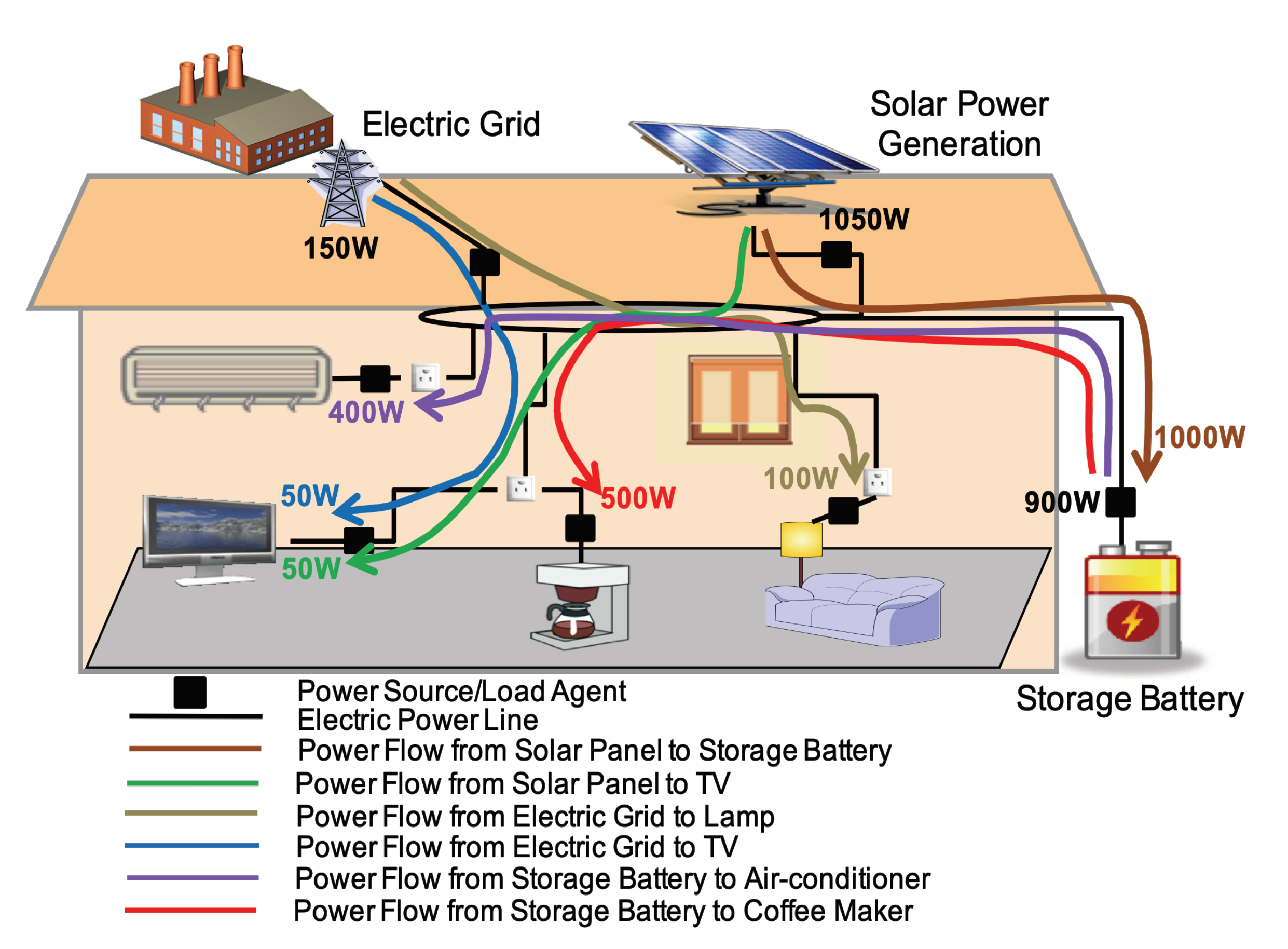
Information technology is currently being used throughout power grids, where embedded smart power sensors, power actuators, and controllers are used for continuous power monitoring, control, and management. Based on the extreme control-ability of smart power devices, the quantity and direction of power stream at each power source and load can be exactly controlled by the power user, which provides the technical foundation for the realization of the sophisticated power flow control. The concept of Power Flow Coloring proposed in [23,24] can be one example of information-technology-supported power flow control. In this concept, individual power flow between a pair of power source and load can be managed with a unique identification attached to each power flow, which enables us to manage versatile power flow patterns between distributed power sources and loads. Figure 1 illustrates the power flow coloring in a household environment.
As mentioned above, one of the most important functions for the power flow control for a power system which contains uncontrollable fluctuating devices and controllable devices is to balance the generated power with the power demand. However, due to the structural limitations, i.e., the power level limitations of controllable sources and loads and the limitation of power flow channels, the power balance may not be achieved. To operate a power system safely under fluctuating environment, the power system must have such property that there always exists a feasible solution, i.e., the power levels for controllable power devices and power flows on connections between power devices which achieve the power balance between power sources and power loads, in any situation of fluctuating devices. We will call such property as “robustness against fluctuation”. This paper discusses structural characteristics for a power system to possess the robustness against fluctuation. This paper proposes two theorems about the structural conditions for a power system to possess the robustness against fluctuation. The first one is a preliminary theorem to the second one, which provides the structural conditions for a power system with given power levels of fluctuating devices to have a feasible control solution. The second one is the main theorem of this paper, which provides the structural conditions for a power system to possess the robustness against fluctuation. The first theorem seems to be more relevant to a control problem which a power flow control needs to solve, while the second and main theorem is more relevant to a power system design, i.e., our main theorem will provide how power sources and power loads should be connected and how large the ability of individual controllable power sources and loads should be, in order to achieve the robustness against power fluctuations caused by fluctuating power devices. The proposed theorem can be applied to any level of power flow system e.g., nano-grid or micro-grid if the connections are incomplete between power sources and loads which is the key point of our research.
The power flow management has been discussed in past with respect to different objectives and optimization techniques [25,26,27,28]. In [29] authors proposed a flexible distributed multi-energy power generation system considering uncertainty for long term. Another research work in [30] studied the multi-energy microgrids considering long term and short-term uncertainty. The main objective of both papers is to enhance demand side flexibility by efficiently using distributed multi-energy generation system. The authors presented a novel approach for power flow management on wide scale using distributed sources and formulate a Multi-Integer Linear Programming (MILP) problem for optimization. However, the system design guidelines and system robustness in the presence of uncertainty caused by fluctuating power devices in real time is not considered which is the main focus of our study. One of the big challenges for integration of renewable energy sources remains in the matching of the intermittent energy generation/production with the dynamic power demand. On the other hand, there are many software packages which can simulate the behavior of a power system, find solutions to constrained optimization problems, etc. However, most of these approaches are based on numerical computations, and it needs intuition and experience of experts as well as repetition of simulation to understand the relation between cause and effect. Compared with these approaches, our approach is not a numerical approach to show the behavior of a given system, rather it explains the reason of existence/inexistence of a solution under power supply/consumption limitation constraints, which will provide us with firm understanding of a power flow system.
This paper is organized as follows: Section 2 describes our structural characterization problem in terms of our system model and power flow control problem is introduced. Section 3 explains our system model which includes representation, and categorization of power devices and connections. Power flow control problem on our system model with fluctuating uncontrollable devices and controllable devices is introduced also in this section. Section 4, is devoted to our first theorem and its mathematical proof, which describes the structural conditions for a power system with given power levels of fluctuating devices to have a feasible control solution. The second and main theorem which describes the structural condition for a power system to possess the robustness against fluctuation is shown in Section 5. Numerical results with illustrative examples of considered system for the application of proposed theorems have been explained in Section 6, Finally, Section 7 gives concluding remarks.
2. Structural Condition Issues and Reasoning
2.1. Incomplete Graph and Its Advantages
Due to the increase in power load demand on the consumer side, fossil energy reserve of electric power system are being exhausted rapidly and resulting in higher energy prices [31]. Despite the intermittent nature, renewable power sources are gaining much consideration than non-renewable energy sources [32]. As for the future energy support, the use of renewable energy technologies is increasing. Hence, it is essential to maximize their profits without losing the stability of the power system.
On the other hand, deregulation of power system is introduced in many countries of the world [33]. Since power demand and its form is changing rapidly, therefore, recognition and determination of most accurate power sources and efficient power transmission are important aspects to consider and long-distance transmission of power from one place to another through multiple buses is another critical point to focus as mentioned in [34]. Undoubtedly, power transmission from one point to another point through multiple power buses causes power loss. Also, the power system stability decreases constantly when the power transmission lines become longer for the long-distance transmission. For the power loss due to a long power transmission line (and conversion loss from one bus to another bus with different characteristics), we need to avoid long-distance (and/or via many different buses) power transmission (except for the case of emergency). For example, if we impose some limitation on the distance (or the number of intermediate buses) of power line transmission, the connection graph is no longer a complete graph (i.e., it must be an incomplete bipartite graph), and a normal operation (except for emergency) is maintained based on this bipartite graph model.
With the increase of power loads of different types (AC loads or DC loads), the DC power network is separated from the AC power network called hybrid AC-DC power network [35,36,37]. In a standard renewable energy connected to AC only power network, the power need to be converted not only once but twice to supply power to DC loads. The DC power supply is first converted to AC power, then transformed to DC power for DC power loads/equipment, which leads to power transformation losses. Another motivation for this type of system is to supply the right power to the right equipment. Separating the power network into DC and AC power network allows the native power to be supplied to the devices optimizing efficiency at every level. Moreover, the complexity of the power flow control problem is high with complete connection graph. In order to mitigate the complexity of power flow control problem, we need to limit the possible connections between power sources and loads.
In [23,24], the concept of the Power Flow Coloring is presented, which attaches the unique ID to each connection between a power source and a load. The concept of the power flow coloring is implemented using real physical devices to show that how power fluctuations are managed with the cooperation of controllable power devices. The power generation excess and shortages are handled by efficiently controlling terminal power devices. In the implementation phase, connections are restricted or reduced to supply power from selected sources to selected loads. This represents the incomplete graph implementation in a household environment. In this research study, the system design guidelines and power device constraints for incomplete connections are studied deeply.
2.2. Problem Discussed in This Paper
We will treat a power system which comprises of power sources, power loads and connections between them. We consider fluctuating power sources/loads as well as controllable power sources/loads, where the last can work for absorbing the fluctuation of power generation/demand in the former and for constructing an entire system robust against the consequences from fluctuating devices.
At each time instance, the power flow control problem with measured information of fluctuating power devices needs to be solved. One of the major objectives of the power flow control is to maintain the balance between generating power and demand. In a real physical situation, the system controller desires to handle power transient behavior, latency of system control, cost efficiency, etc. However, the issue whether the power flow system (i.e., power flow control problem) has a feasible solution in terms of power balance or not is one of the most important issues.
If we consider a complete connection between power sources and power loads, i.e., each power source can provide the power to every individual power load, the condition for a feasible solution in terms of power balance might be trivial as, , and . The first inequality means that the (total) amount of generated power by fluctuating power source(s) can be consumed completely by the (total) demand of fluctuating load(s) and by controlling controllable power load(s) with the maximum available consuming power . On the other hand, the second inequality means that the (total) demand of fluctuating loads(s) can be fully satisfied by the (total) generating power of fluctuating source and by controlling controllable power source(s) with the maximum available power . However, if the connection between sources and loads is incomplete, i.e., for some pairs of source and load, there is no transfer mechanism/route by which the power is transmitted from a source to a load, the solvability issue is not trivial. In this paper, we will discuss the issue of power balance under such an incomplete connection between sources and loads.
If we use some numerical tool to compute the solution of problem, we can know existence/inexistence of a feasible solution for each individual instance of the problem. However, our approach discussed in this paper is different from it.
Our concern is the structural condition which makes the power flow control problem solvable in terms of power balancing, i.e., how power sources and power loads should be connected and how large the ability of individual controllable power sources and loads should be in order for a power flow system to have a feasible solution of the power flow control problem. Hence, the major application area of our results in this paper is the design issue of a power flow system, since the allocation of power sources and power loads, the connections (power flow channels) between power sources and loads, and the capacity of individual power sources and loads need to be designed so that the resultant power flow system always has a feasible solution under any situation of fluctuating power devices (this property is called “robustness against fluctuation”).
In the following of this paper, we will discuss two types of system conditions. The first one is the structural condition for a power flow system with given power levels of fluctuating devices to have a feasible solution of the power flow control problem, and the second one is the structural condition for a power flow system to possess the robustness against fluctuation. As a first attempt to investigate structural conditions for a power flow system to possess the robustness against fluctuation, the connectivity of connections between power sources and loads and the maximum and the minimum power levels of individual power devices are considered to be structural factors, and the capacity of individual connections is assumed to be large enough so that it does not affect the existence/inexistence of a feasible solution of the power flow control problem. The improved structural conditions regarding the capacity of individual connections remain as a future problem.
In this paper, we do not consider any specific target level of a power network, but aim to provide a general discussion about the power balancing under an incomplete connection between power sources and loads.
3. System Model
This section describes the details of our system model and explains the Power Flow Control Problem.
3.1. Representation and Categorization of Power Devices
This subsection shows the representation of power devices with both types and connections between them as given in Figure 2.
A power source can be defined as an electric device which can supply electric power to electric loads, e.g., photovoltaic, wind turbine, utility grid, etc. A power load is an electric device which consumes electric power supplied by power sources. All power devices (i.e., sources and loads) are divided into two categories based on their characteristics and functionality, such as Controllable and Fluctuating . A controllable can control its power (supply/consume), whereas fluctuating cannot control its power.
All power sources with both types will be represented as, , where I and J show the total numbers of controllable and fluctuating power sources, respectively. Similarly, all power loads will be indexed as, where K and L show the total numbers of controllable and fluctuating power loads. For convenience sake, we will use for representing the set of controllable power devices in a set •, and for representing the set of fluctuating devices in a set •.
A power agent is attached to each , which measures and controls the power levels of the attached power device. The actual power levels (i.e., generation and consumption) of sources and loads will be represented as , , and , respectively for , , and .
Each device has a minimum power level and maximum power level limitation, which represents the range of power modes/operation and performance of that particular device. The minimum power supply/generation limit and maximum limit show the capacity of a controllable source and the power generated by is assumed to be bounded as,
Similarly, the minimum and maximum power generation limits will be given as and respectively, for and the power generation is limited as,
For the power demand of controllable load with given minimum and maximum levels and , and for the power demand of fluctuating load with given minimum and maximum levels and are bounded as,
3.2. Connections between Power Sources and Power Loads
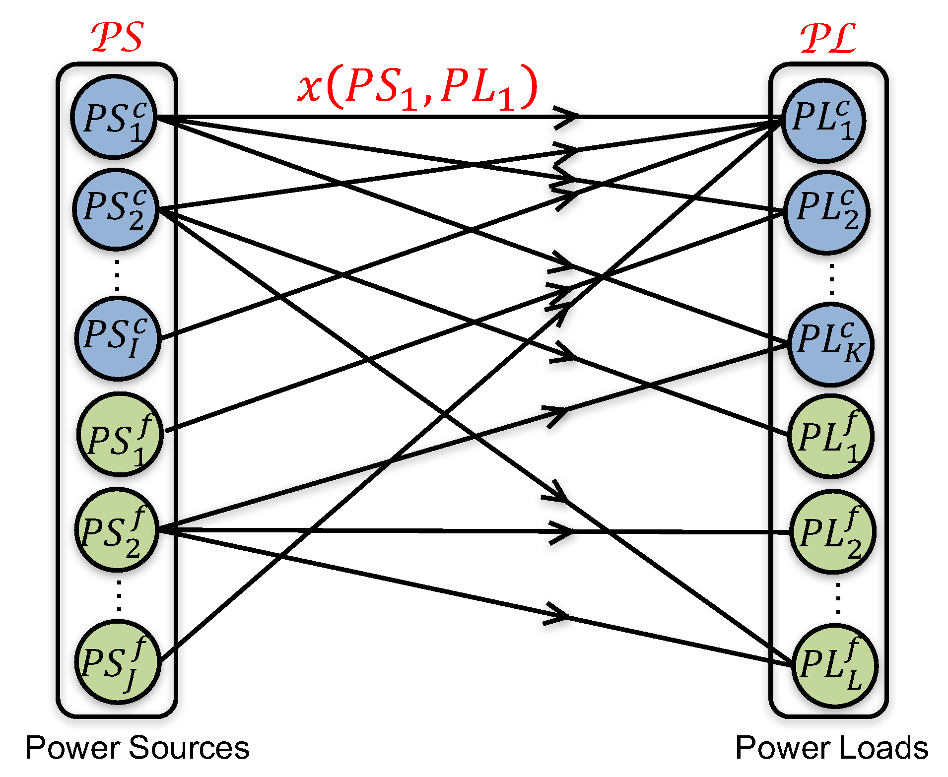
A connection is a pair of a PS and a PL, . The real physical arrangement of power devices and connection between them can be modeled with a bipartite graph which is introduced in Figure 3.
The system model considered in this paper thus consists of a set of power sources , a set of power loads , and a set of connections between power sources and loads as, . The system model represents the incomplete connections between power sources and loads and the connection in this figure shows the power transfer/supply from power source to load. Power devices without connection show that there is no possibility of power transfer/supply between power devices. The key point of the paper is the consideration of between devices.
In Figure, power devices with each type are represented with different colors. Each connection is associated with some power level in Watt to show the amount of power supplied from a source to a load via this connection, which is assumed to be always non-negative real number.
3.3. Power Flow Control Problem
As the actual/physical power by a fluctuating power device changes a lot due to its type of device and operation mode, the power stream on each power flow/connection must be altered according to the fluctuating situation. Here, it is supposed that the power levels of fluctuating power devices are noted with smart power sensors for each time instance. In order to adjust power fluctuations triggered by fluctuating power devices, a power flow control is essential. This power flow control method uses measured power levels of fluctuating power devices and calculates power levels for controllable power devices and connections under the power balance restriction such that the total power supplied/generated by all power sources is fully used by power loads, and all power loads take sufficient power from power sources.
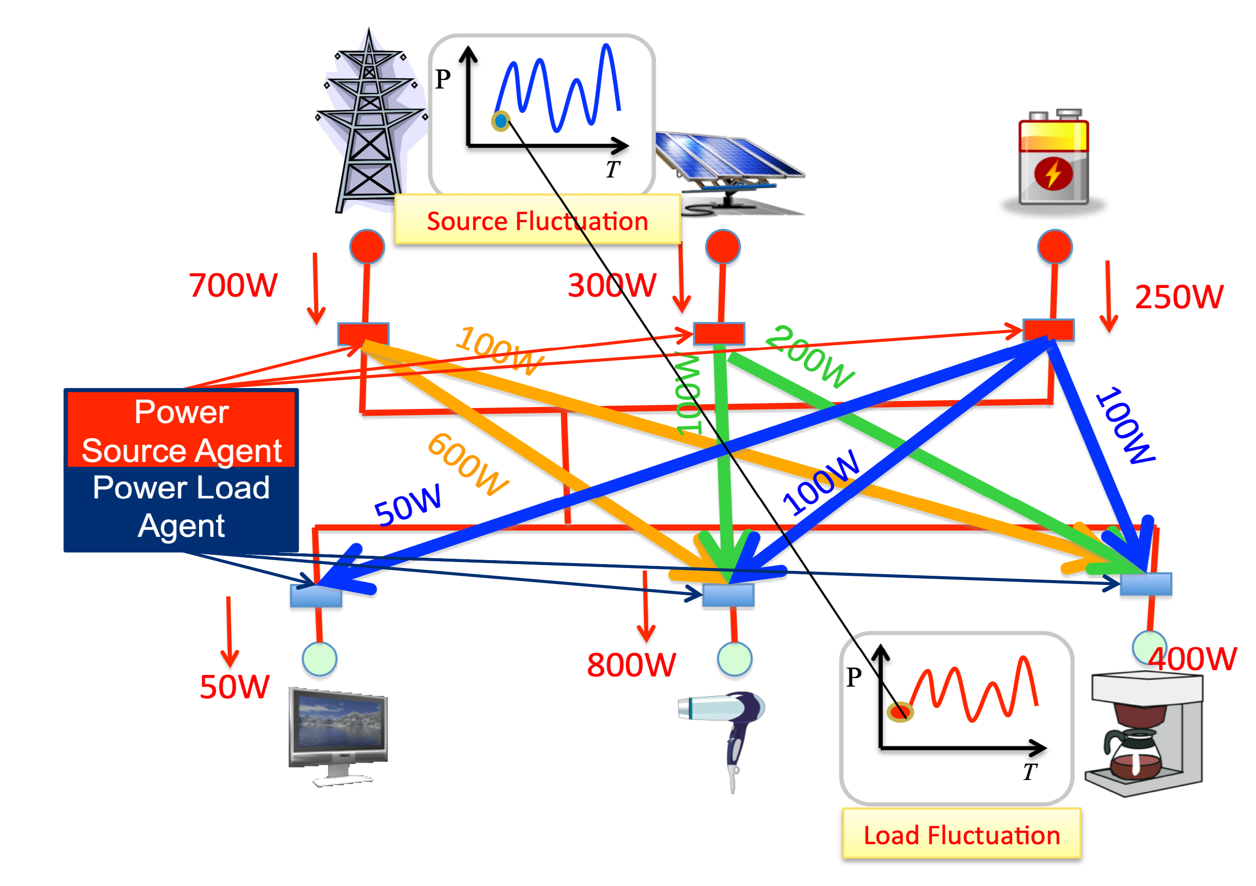
Each connection connects a to its neighbor on the other side of the connection. The set of neighbors of is denoted as , which can be separated into and , the sets of controllable and fluctuating power devices, respectively. As for the representation of neighboring devices and the power flows, please refer to Figure 4.
The sum of all outgoing power flows, , of power source can be written as,
Similarly, the sum of all incoming flows, , of a power load, , can be computed as,
At the end of power flow control in each time instance, the power generation of power source must be equal to the sum of all outgoing flows, as,
and the power consumption of power load must be equal to the sum of all incoming power flows to this PL as,
Therefore, the ultimate goal of this proposed power control problem is, for given (measured) power levels and of fluctuating power sources and loads, find the power levels and of controllable power sources and loads and power flow assignment such that (5) and (6) are satisfied along with the limitations given by (1) and (3). Since we can control and freely while keeping individual minimum and maximum power limitations for each power device, the problem can be considered to be to find such that
4. System Condition with Given Power Levels for Fluctuating Power Devices
First we consider a general instance of the power flow control problem where the generated power levels and demand levels for fluctuating power sources and loads, respectively, are given as constant values (values obtained by measurement), and provide the structural condition for this problem instance to have a feasible solution (Theorem 1). The structural conditions described in Theorem 1 can be an important base for our main theorem (Theorem 2 shown in the next section) which provides the structural conditions for a system to possess the robustness against fluctuation, i.e., the conditions for a system to have a feasible solution of the power flow control problem for any power levels of fluctuating power devices.
Theorem 1.
The power flow control problem can find the feasible solution if and only if the following two system conditions are satisfied.
Condition 1-1:
Condition 1-2:
Proof of Theorem 1.
First, we introduce the necessity of the system conditions. Let be a feasible solution of power flow control problem and let S be an random subset of power sources, then (5) and (6) are satisfied for every and , which further yields the following equations.
and
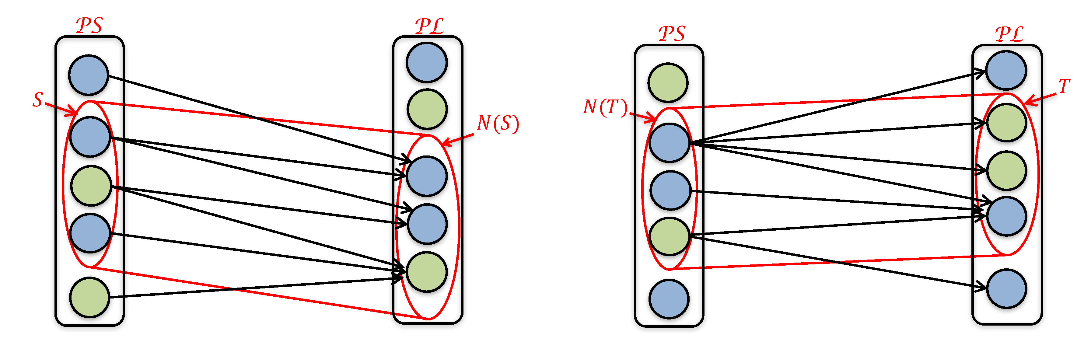
Since each power source in S is supplying power to power loads in , but the power loads in can receive power from other power sources not in S (see Figure 5a), we can have the following inequality,
On the other side, the total summation of all outgoing power streams from power sources in S can be written as,
Similarly, the total incoming power flows into can be represented as,
By combining (11)–(13), we can conclude that Condition 1-1, is satisfied whenever the system has a feasible solution. The necessity of Condition 1-2 can be presented in a same way, in which the following inequality is a key to show such situation.
The above inequality holds since each power load in T is getting power from power sources in , but the power sources in can give power to loads not in T. □
To provide the sufficiency, we will introduce several definitions and an auxiliary optimization problem generated from our original power flow control problem. The goal of this sufficiency proof is, supposing that Condition 1-1 and Condition 1-2 are satisfied, to show the “existence” of a feasible solution of our original power flow control problem, i.e., a power flow assignment which satisfies (7)–(10). The following definitions and an auxiliary optimization problem are introduced for this purpose.
Definition 1.
Each power source could have three states: Power-High, Power-Low, and Power-Balanced.
Power-High: When holds for a controllable power source , there is room to increase the outgoing power flow . Such power source is called “power-high” node. Similarly, when for a fluctuating power source , is also called “power-high” node.
Power-Low: When holds for , there is room to decrease outgoing power flow . Such power source is called “power-low” node. Similarly, when for , is also called “power-low” node.
Power-Balanced: When holds for , we can control the power level of so that the generating power and the outgoing power are balanced. Such is called “power-balanced” node. Similarly, when for , is called “power-balanced” node.
According to the above definition, a controllable power source with is power-high, power-low and power-balanced simultaneously. It means, for such power source, the outgoing power can be increased (“power-high”), decreased (“power-low”) or kept unchanged (“power-balanced”) by controlling the generating power level of within its minimum and maximum power limits. On the other hand, the definitions of power-high, power-low and power-balanced for a fluctuating power source are disjoint, since the generating power level is given and cannot be altered for a fluctuating power source, and power-balanced state needs exactly.
Three states, power-high, power-low and power-balanced, are defined also for a power load as follows.
Power-High: When holds for a controllable power load , or for fluctuating power load , there is room to decrease the incoming power flow or , respectively. Such power load is called “power-high” node.
Power-Low: When holds for , or for , there is room to increase the incoming power flow or , respectively. Such power load is called “power-low” node.
Power-Balanced: When holds for , or for , such power lord is called “power-balanced” node.
Similar to the definitions for a power source, the definitions of these three states for a controllable power load are overlapped, while they are not overlapped for a fluctuating power load.
Definition 2.
A power path is an alternative sequence of devices/nodes and power flows/connections, where each device in a path is either an initial node followed by a power flow/connection incident to this device, an intermediate device which is incident to the previous and the following power flow/connections or a finishing device which is incident to the previous connection. A power path can contain “forward edges” with similar direction with path direction and “backward edges” with the reverse direction with the power path direction. If every backward edge has increment in the power flow amount, then the power path is called “alternating path”. The power flow obligation on each flow/connection of an alternating path is shown in Figure 6.
Definition 3.
An alternating power path which initialize from “power-high” device/node and ends/terminates on “power-low” device is called an augmenting path (Figure 7).
Definition 4.
With regard to an augmenting path, the procedure to increase power flow or amount of power on each connection in the path uniformly by ( for a forward edge, and for a backward edge) is called “power flow augmentation”. Please note that by this power flow management/augmentation, the total incoming/outgoing power of each device/node changes only at an initial device and an ending device.
Please note that the words “alternating path” and “augmenting path” are borrowed from Graph Theory. In addition, our Theorem-1 can be considered to be an extension of Hall’s theorem in Bipartite Matching [38].
Our proof of the sufficiency of Theorem-1 begins with the introduction of the following Optimization Problem-1.
Optimization Problem-1: Find such that
where
with following constraints,
Our goal of this proof is to show that if Conditions 1-1 and 1-2 are satisfied, Optimization Problem-1 always has an optimum solution which makes the objective function zero, i.e.,
It is clear that this type of optimum solution is a feasible solution of our original Power Flow Control Problem.
Please note that since for all is a feasible solution for Optimization Problem-1, there always exists an optimum solution of Optimization Problem-1.
To achieve our goal by contradiction, we assume that the optimum solution does not achieve the objective function equal to zero. This shows that there exists such that or or there exists such that or .
Case 1.
In case such that or exists:
Let A be the group/set of power sources and B be the group/set of power loads which can be extended from by alternating paths. As an alternating path can be stretched from a power source device/node to a power load device/node without any constraint, holds. Conversely, power loads in B can have connection (that must be a zero-power flow) with power sources not exists in A, i.e., . The power used by power loads in B is provided by power sources in A, since power flows amount on connections from to B are zero (see Figure 8), which means . Now we can consider possibilities as given below.
[Case 1-1]: A includes a “power-low” node or B includes a “power-low”:If is a “power-low” node, The alternating path from to (, respectively) is an augmenting path, and the power flow augmentation is applied to get a new power flow assignment which has the difference or smaller than , while none of the other differences , , and becomes larger than that in . It means that the new power flow assignment is a better solution that , which contradicts the optimality of .
[Case 1-2]: Neither A nor B includes “power-low” node:Every node in A and B is either “power-balanced” or “power-high”, which means
Together with the fact that also exists in A, we have,
which is the contradiction to Condition 1-1.
Case 2.
In case such as or exists:
Now, let D and E be the sets of power loads and sources, respectively, which can be a starting node of an alternating path terminating at . Since a starting node of an alternating path can be reached from a load to a source without any restriction, holds. The sources in E can have connection (must have zero-power flow) with power loads outside D, i.e., (see Figure 9). The power generated by power sources in E is supplied to only power loads in D, which means . We can consider the following two possibilities.
[Case 2-1]: D includes “power-high” node or E includes “power-high” node:We can find augmenting path starting from a “power-high” node or and terminating at , and apply the power flow augmentation along this augmenting path to get a new power flow assignment which is better than the assumed optimum solution . It is the contradiction to the assumption.
[Case 2-2]: Neither D nor E includes “power-high” node:Every node in D and E is either “power-balanced” or “power-low” node, which means,
Together with the fact that also exists in C, we have,
which is the contradiction to Condition 1-2.
As stated above, if we assume that the optimum solution of Optimization Problem-1 does not make the objective function zero, it always incurs a contradiction. Hence, if Conditions 1-1 and 1-2 are satisfied, Optimization Problem-1 always has an optimum solution which makes the objective function zero, and hence our original Power Flow Control Problem has a feasible solution.
5. System Condition for the Robustness against Fluctuation
In this section, we assume that each fluctuating power device has an arbitrary power level within the specified minimum and maximum levels. Even though the power level of individual fluctuating device is not specified as a concrete number, we can guarantee the existence of a feasible solution of the power flow control problem if some structural conditions are satisfied. The following Theorem 2 describes these structural conditions.
Theorem 2.
The power flow control problem continuously has a feasible solution if and only if the succeeding two conditions are fulfilled.
Condition 2-1:
Condition 2-2:
Proof of Theorem 2.
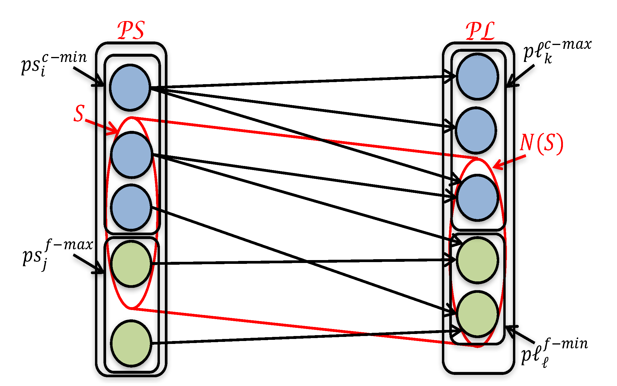
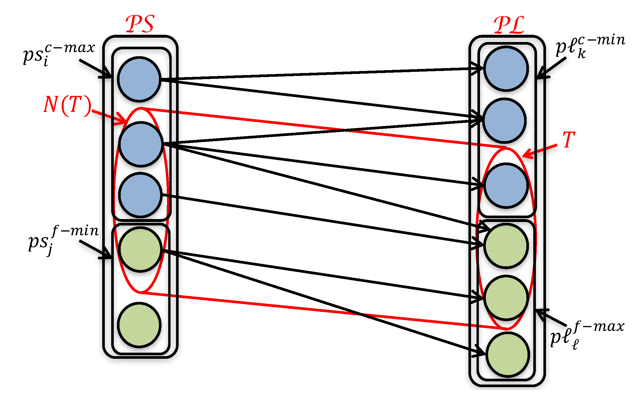
Here, we presented the sufficiency of above system conditions. Let S be any group/subset of power sources and be the connected/neighbor set of S (see Figure 10), then from Condition 2-1, Condition 1-1 can be held as,
This determines that if the system Condition 2-1 is satisfied, then system Condition 1-1 is always satisfied for any power level generated/consumed of fluctuating power devices. Correspondingly, for any group/subset of power loads T and its connected/neighbor group/subset of power sources (see Figure 11), Condition 1-2 can be obtained as,
This proves that Condition 2-2 is satisfied, then Condition 1-2 is always fulfill for any situation of fluctuating power devices.
A system, which has a feasible solution for any situation of fluctuating devices, must have a feasible solution even for the case and for all fluctuating devices. From the necessity of Condition 1-1 with this specific situation of fluctuating devices, the necessity of Condition 2-1 is shown. Similarly, considering the necessity of Condition 1-2 for a specific case with and , the necessity of Condition 2-2 is shown. □
6. Numerical Results
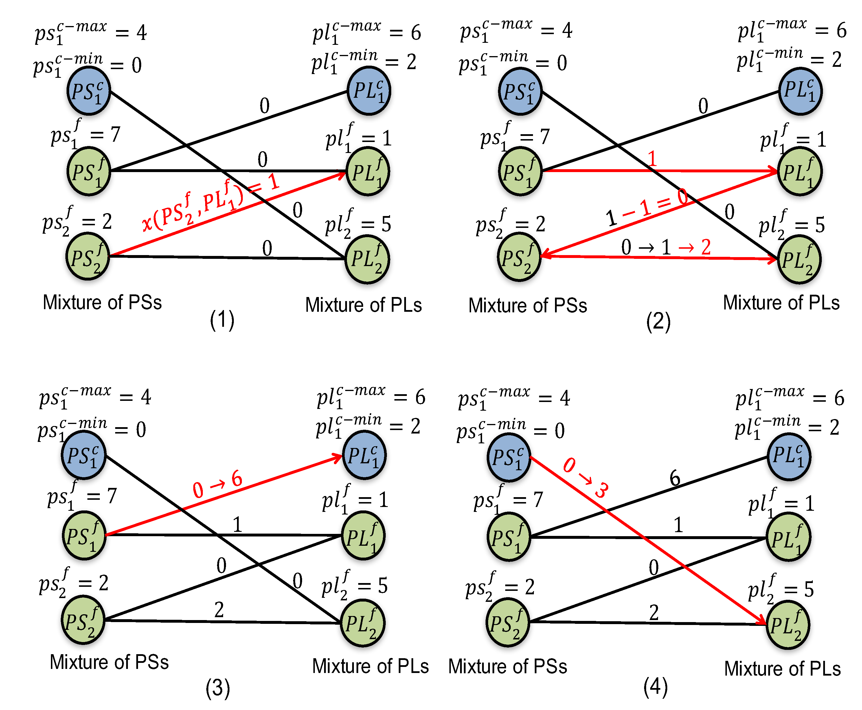
This subsection signifies the application of the proposed theorem to demonstrate the existence of a feasible solution. We design the system with three power suppling devices and three power consuming devices with connections. One power sources is chosen as controllable , and the remaining two sources are chosen as fluctuating and . Likewise, one of the load is chosen as controllable , and remaining two loads are fluctuating as and .
In Figure 12, given power levels by fluctuating power sources are represented as, , and . The power request levels by fluctuating loads are indicated as, , and , respectively. The controllable power devices are restricted between power limitations i.e., maximum and minimum power limits as, , and, . The power boundaries for controllable load are given as, , and . At first, we demonstrate that Condition 1-1 is fulfilled for all subsets of power sources.
Table 1 indicates all possible subsets of power sources with connected/neighbor subsets with power generation and consumption calculation according to Condition 1-1. For each subset, the summation of minimum power levels for controllable and given power levels of fluctuating is less or equal to the sum of maximum power levels for controllable load and given power levels for fluctuating loads. Similarly, we can represent that the Condition 1-2 is also fulfilled and finally we discover that the system fulfilled conditions 1-1 and 1-2, and we have feasible solution.
As for the power flow allocation for each connection, first it is considered to be “zero”. Since all sources are “power-high”, the system will try to find an augmenting path to increase power by choosing a source randomly. For example, the augmenting path commenced with and ended at “power-low” node is chosen and the power is increased on this connection by “1” to satisfy the power demand (Figure 12(1)). This makes this power load a “power-balanced” node. Also, we select a path from to and augmented power flow by “1”. The next augmenting path is chosen from to through and and power flow along this path is augmented by “1” so that the power flow on each connection does not become negative as displayed in the Figure 12(2). Since and became “power-balanced” nodes, the next augmenting path is chosen from to for power increase by “6” (Figure 12(3)). Now all power devices are “power-balanced” except and , so system chosen augmenting path starting from and ending at to increase power by “3” (Figure 12(4)). Here, we select generated power by fluctuating power devices as much as possible to keep power supply of controllable power sources.
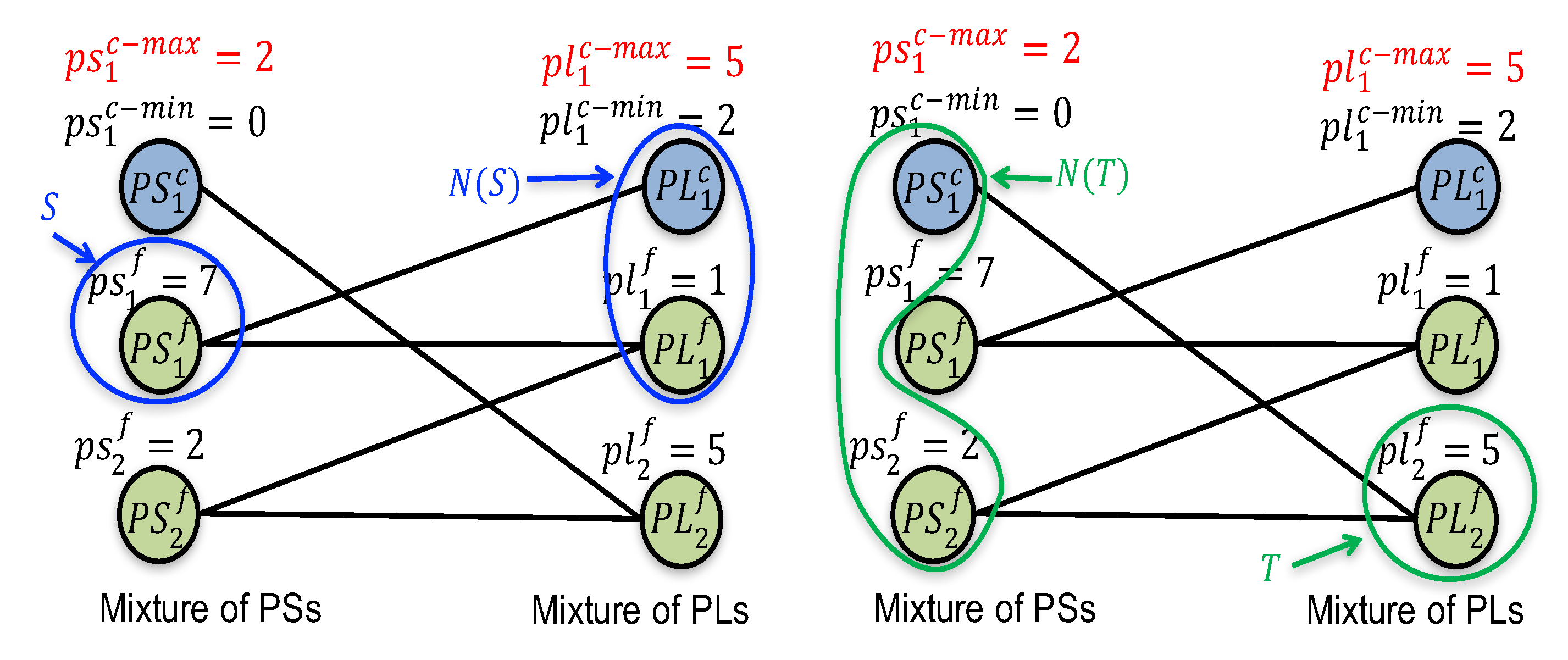
In Figure 13, non-feasible case is discussed. The power supply and consumption levels for fluctuating power devices are same with the previous example but the maximum power levels for controllable sources and loads are different. We observed that by changing the maximum power limits, the conditions 1-1, and 1-2 are not satisfied for subsets S, and T and their neighboring devices shown in Figure 13. For this case, we cannot find the feasible solution for the given system.
7. Concluding Remarks
Renewable energy sources such as wind power and photovoltaic power generation system play very important roles because of low impact against the environment. However, the generated power from the renewable energy sources varies greatly, resulting in a risk of fluctuations which is uncontrollable. The increased penetration of renewable energy sources has an effect on the power system’s stability and quality of power. In addition, the power fluctuations caused by power loads also have the same consequences on power system. From such point of view, in which power supply and demand changes dynamically, a power flow control mechanism is introduced which assigns power levels for controllable power devices and connections between power devices to absorb the power fluctuations caused by fluctuating devices.
In order for a power system to continue a safe operation under the presence of fluctuating power levels of fluctuating devices, the power flow control algorithm should be designed properly and, at the same time, a power system itself should be designed properly. This paper proposed structural system conditions for a power system to possess the robustness against fluctuation, i.e., the condition for a system to have always a feasible solution of the power flow control problem with any power levels of fluctuating devices (Theorem 2). These conditions are described in terms of the connectivity of connections between power sources and loads and the minimum and the maximum power levels of individual power devices. Most important application area of our result might be a power system design which includes the allocation of power devices, allocation of connections between power devices, and specification of the maximum and the minimum power levels of individual power devices.
As a first attempt to investigate structural conditions for a power flow system to possess the robustness against fluctuation, we have discussed the power flow control problem and structural conditions based on a relatively simple system model. For example, the capacity of individual connections is assumed to be large enough so that it does not affect the existence/inexistence of a feasible solution of the power flow control problem. The improved structural conditions regarding more sophisticated system model, e.g., consideration of the capacity of individual connections, and the limitation of speed of change in power levels of power devices remain as future problems.
Author Contributions
Conceptualization, S.J., M.K., and Y.T.; writing—original draft preparation, S.J.; writing—review and editing, S.J., and M.K.; supervision, M.K., and Y.T. All authors have read and agreed to the published version of the manuscript.
Funding
This research received no external funding.
Conflicts of Interest
The authors declare no conflict of interest.
References
- Maegaard, P. Balancing fluctuating power sources. In Proceedings of the World-Non-Grid-Connected Wind Power and Energy Conference, Kunming, China, 13–17 October 2010. [Google Scholar]
- Soroudi, A.; Ehsan, M.; Caire, R.; Hadjsaid, N. Possibilistic evaluation of distributed generations impacts on distribution networks. IEEE Trans. Power Syst. 2011, 26, 2293–2301. [Google Scholar] [CrossRef] [Green Version]
- Umer, S.; Tan, Y.; Lim, A.O. Stability analysis for smart homes energy management system with delay consideration. J. Clean Energy Technol. 2014, 2, 332–338. [Google Scholar] [CrossRef]
- Umer, S.; Tan, Y.; Lim, A.O. Priority based power sharing scheme for power consumption control in smart homes. Int. J. Smart Grid Clean Energy 2014, 3, 340–346. [Google Scholar] [CrossRef] [Green Version]
- Umer, S.; Kaneko, M.; Tan, Y.; Lim, A.O. System design and analysis for maximum consuming power control in smart house. J. Autom. Control Eng. 2014, 2, 43–48. [Google Scholar] [CrossRef]
- Lumbreras, S.; Ramos, A.; Banez-Chicharro, F. Optimal transmission network expansion planning in real-sized power systems with high renewable penetration. Electr. Power Syst. Res. 2017, 149, 76–88. [Google Scholar] [CrossRef]
- Han, J.; Choi, C.; Park, W.; Lee, I.; Kim, S. Smart home energy management system including renewable energy based on ZigBee and PLC. IEEE Trans. Consum. Electron. 2014, 60, 198–202. [Google Scholar] [CrossRef]
- Han, J.; Choi, C.; Park, W.; Lee, I.; Kim, S. PLC-based photovoltaic system management for smart home energy management system. IEEE Trans. Consum. Electron. 2014, 60, 184–189. [Google Scholar] [CrossRef]
- Hong, I.; Kang, B.; Park, S. Design and implementation of intelligent energy distribution management with photovoltaic system. IEEE Trans. Consum. Electron. 2012, 58, 340–346. [Google Scholar] [CrossRef]
- Rashidi, Y.; Moallem, M.; Vojdani, S. Wireless Zigbee system for performance monitoring of photovoltaic panels. In Proceedings of the 2011 37th IEEE Photovoltaic Specialists Conference, Seattle, WA, USA, 19–24 June 2011; pp. 3205–3207. [Google Scholar]
- Xiaoli, X.; Daoe, Q. Remote monitoring and control of photovoltaic system using wireless sensor network. In Proceedings of the 2011 International Conference on Electric Information and Control Engineering, Wuhan, China, 15–17 April 2011; pp. 633–638. [Google Scholar]
- Biabani, M.; Golkar, M.A.; Johar, A.; Johar, M. Propose a home demand -side management algorithm for smart nano-grid. In Proceedings of the 4th Annual International Power Electronics, Drive Systems and Technologies Conference, Tehran, Iran, 13–14 February 2013; pp. 487–494. [Google Scholar]
- Asare-Bediako, B.; Kling, W.L.; Robeiro, P.F. Home energy management systems: Evolution, trends and frameworks. In Proceedings of the 2012 47th International Universities Power Engineering Conference (UPEC), London, UK, 4–7 September 2012; pp. 1–5. [Google Scholar]
- Shwehdi, M.H.; RajaMuhammad, S. Proposed smart DC Nano-Grid for green buildings a reflective view. In Proceedings of the 2014 International Conference on Renewable Energy Research and Application (ICRERA), Milwaukee, WI, USA, 19–22 October 2014; pp. 765–769. [Google Scholar]
- Kinn, M.C. Proposed components for the design of a smart Nano-Grid for a domestic electrical system that operates at below 50V DC. In Proceedings of the IEEE PES International Conference and Exhibition on Innovative Smart Grid Technologies (ISGT Europe), Manchester, UK, 5–7 December 2011; pp. 1–7. [Google Scholar]
- Schonberger, J.; Duke, R.; Round, S.D. DC-Bus signaling: A distributed control strategy for a hybrid renewable Nano-grid. IEEE Trans. Ind. Electron. 2006, 53, 1453–1460. [Google Scholar] [CrossRef]
- Latha, S.H.; Mohan, S.C. Centralized power control strategy for 25 kW Nano-Grid for rustic electrification. In Proceedings of the 2012 International Conference on Emerging Trends in Science, Engineering and Technology (INCOSET), Tiruchirappalli, India, 13–14 December 2012; pp. 456–461. [Google Scholar]
- Kondoh, J.; Higuchi, N.; Sekine, S.; Yamaguchi, H.; Ishii, I. Distribution system research with an analog simulator. In Proceedings of the First Industrial Conference on Power Electronics for Distributed and Co-generation, Irvine, CA, USA, 22–24 March 2004. [Google Scholar]
- Kondoh, J.; Aki, H.; Yamaguchi, H.; Murata, A.; Ishii, I. Consumed power control of time deferrable loads for frequency regulation. In Proceedings of the IEEE PES Power Systems Conference and Exposition, New York, NY, USA, 10–13 October 2004. [Google Scholar]
- Okabe, Y.; Sakai, K. QoEn (Quality of Energy) Routing toward Energy on Demand Service in the Future Internet; ICE-IT, Academic Center for Computing and Media Studies, Kyoto University: Kyoto, Japan, 2009. [Google Scholar]
- Abe, R.; Taoka, H.; McQuilkin, D. Digital Grid: Communicative electrical grids of the future. IEEE Trans. Smart Grid 2011, 2, 399–410. [Google Scholar] [CrossRef]
- Takuno, T.; Kitamori, Y.; Takahashi, R.; Hikihara, T. AC power routing system in home based on demand and supply utilising distributed power sources. Energies 2011, 4, 717–726. [Google Scholar] [CrossRef] [Green Version]
- Javaid, S.; Kurose, Y.; Kato, T.; Matsuyama, T. Cooperative distributed control implementation of the power flow coloring over a Nano-grid with fluctuating power loads. IEEE Trans. Smart Grid 2017, 8, 342–352. [Google Scholar] [CrossRef]
- Javaid, S.; Kato, T.; Matsuyama, T. Power flow coloring system over a Nano-grid with fluctuating power sources and loads. IEEE Trans. Ind. Inform. 2017, 13, 3174–3184. [Google Scholar] [CrossRef]
- Yamaguchi, H.; Kondoh, J.; Aki, H.; Murata, A.; Ishi, I. Power fluctuation analysis of distribution network introduced a large number of photovoltaic generation system. In Proceedings of the 18th International Conference and Exhibition on Electricity Distribution, Turin, Italy, 6–9 June 2005. [Google Scholar]
- Riffonneau, Y.; Bacha, S.; Ploix, S. Optimal power flow management for grid connected PV systems with batteries. IEEE Trans. Sustain. Energy 2011, 2, 309–320. [Google Scholar] [CrossRef]
- Denholma, P.; Margolis, R.M. Evaluating the limits of solar pho-tovoltaics (PV) in electric power systems utilizing energy storage and other enabling technologies. Energy Policy 2007, 35, 4424–4433. [Google Scholar] [CrossRef]
- Perrin, M.; Saint-Drenan, Y.M.; Mattera, F.; Malbranche, P. Lead- acid batteries in stationary applications: Competitors and new markets for large penetration of renewable energies. J. Power Sources 2005, 144, 402–410. [Google Scholar] [CrossRef]
- Cesena, E.A.M.; Capuder, T.; Mancarella, P. Flexible distributed multienergy generation system expansion planning under uncertainty. IEEE Trans. Smart Grid 2016, 7, 348–357. [Google Scholar] [CrossRef]
- Wei, J.; Zhang, Y.; Wang, J.; Cao, X.; Khan, M.A. Multi-period planning of multi-energy microgrid with multi-type uncertainties using chance constrained information gap decision method. Appl. Energy 2020, 260, 1–19. [Google Scholar] [CrossRef]
- Garcez, C.G. Distributed electricity generation in Brazil: An analysis of policy context, design and impact. Util. Policy 2017, 49, 104–115. [Google Scholar] [CrossRef]
- Sharma, P.; Tandon, A. Techniques for optimal placement of DG in radial distribution system: A review. In Proceedings of the Communication, Control and Intelligent Systems (CCIS), Mathura, India, 7–8 November 2015; pp. 453–458. [Google Scholar]
- Kazemi, A.; Bayat, P.M. Determination and allocation of reactive power loss in deregulated power systems in the presence of multilateral multiple contracts. In Proceedings of the International Conference on Power Engineering, Energy and Electrical Drives, Setubal, Portugal, 12–14 April 2007; pp. 454–459. [Google Scholar]
- Caampued, C.P.C.C.; Aguirre, R.A. Determination of penetration limit of wind distributed generation considering multiple bus integration. In Proceedings of the IEEE Asia-Pacific Power and Energy Engineering Conference (APPEEC), Kota Kinabalu, Malaysia, 7–10 October 2018; pp. 370–375. [Google Scholar]
- Ebrahim, A.F.; Youssef, T.A.; Mohammed, O.A. Power quality improvements for integration of hybrid AC/DC nanogrids to power systems. In Proceedings of the IEEE Green Technologies Conference, Denver, CO, USA, 29–31 March 2017; pp. 171–176. [Google Scholar]
- Egghtedarpour, N.; Farjah, E. Power control and management in a hybrid AC/ DC microgrid. IEEE Trans. Smart Grid 2014, 5, 1494–1505. [Google Scholar] [CrossRef]
- Nejabatkhah, F.; Li, Y.W. Overview of power management strategies of hybrid AC/DC microgrid. IEEE Trans. Power Electron. 2015, 30, 7072–7089. [Google Scholar] [CrossRef]
- Axler, S.; Ribet, K.A. Graduate Texts in Mathematics; Springer: Berlin, Germany, 2008. [Google Scholar]
Figure 1.
The concept of The Power Flow Coloring.

Figure 2.
Representation of power sources, power loads, and connections between them.

Figure 3.
Representation of power sources, power loads, and connections between them using bipartite graph.
Figure 3.
Representation of power sources, power loads, and connections between them using bipartite graph.

Figure 4.
Connections between Power Sources and Power Loads. (a) A power source with connections; (b) A power load with connections.
Figure 4.
Connections between Power Sources and Power Loads. (a) A power source with connections; (b) A power load with connections.

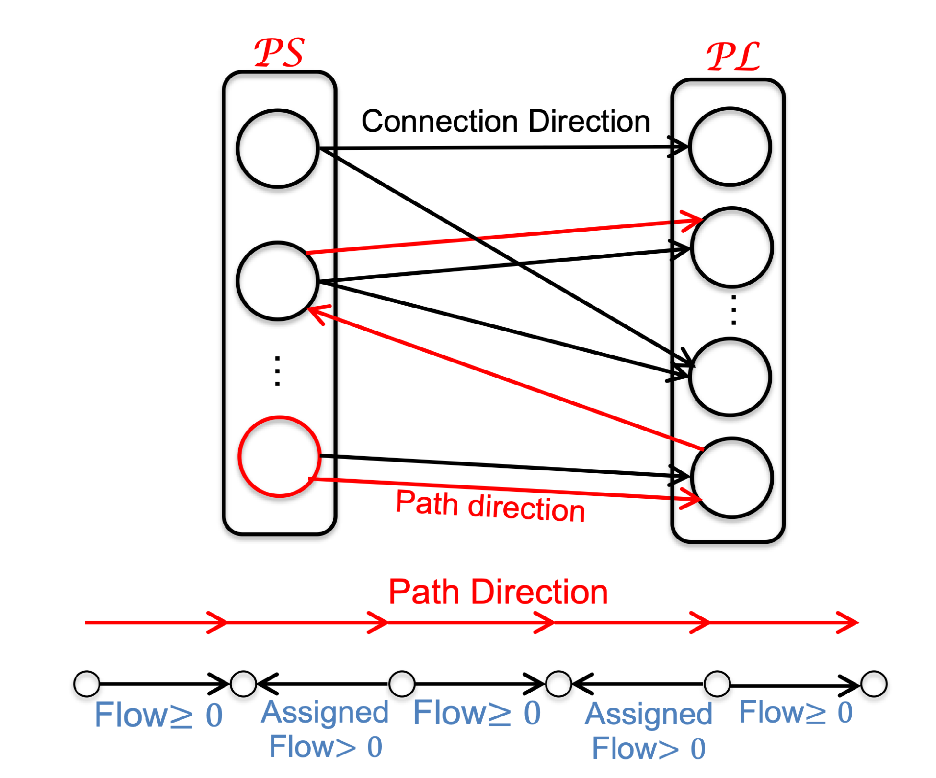
Figure 5.
Illustration of subsets of power sources and loads. (a) Subset S of power sources and neighbor/connected set ; (b) Subset T of power loads and its neighbor/connected set .
Figure 5.
Illustration of subsets of power sources and loads. (a) Subset S of power sources and neighbor/connected set ; (b) Subset T of power loads and its neighbor/connected set .

Figure 6.
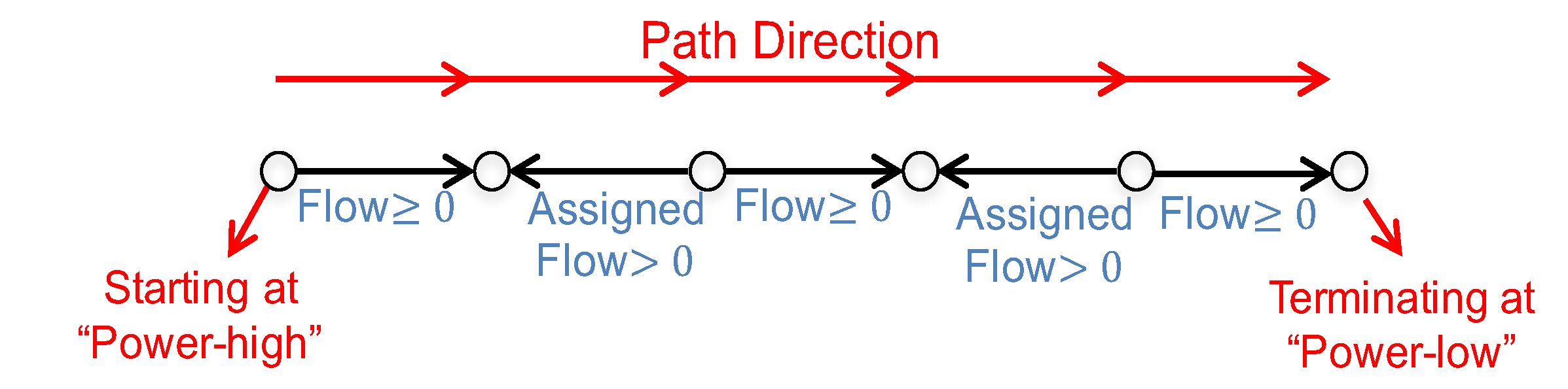
Alternating Path.

Figure 7.
Augmenting Path.

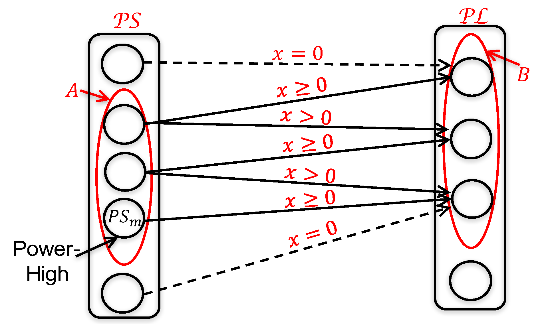
Figure 8.
Illustration of sets A and B of power sources and power loads, respectively, which are reachable from by alternating paths.
Figure 8.
Illustration of sets A and B of power sources and power loads, respectively, which are reachable from by alternating paths.

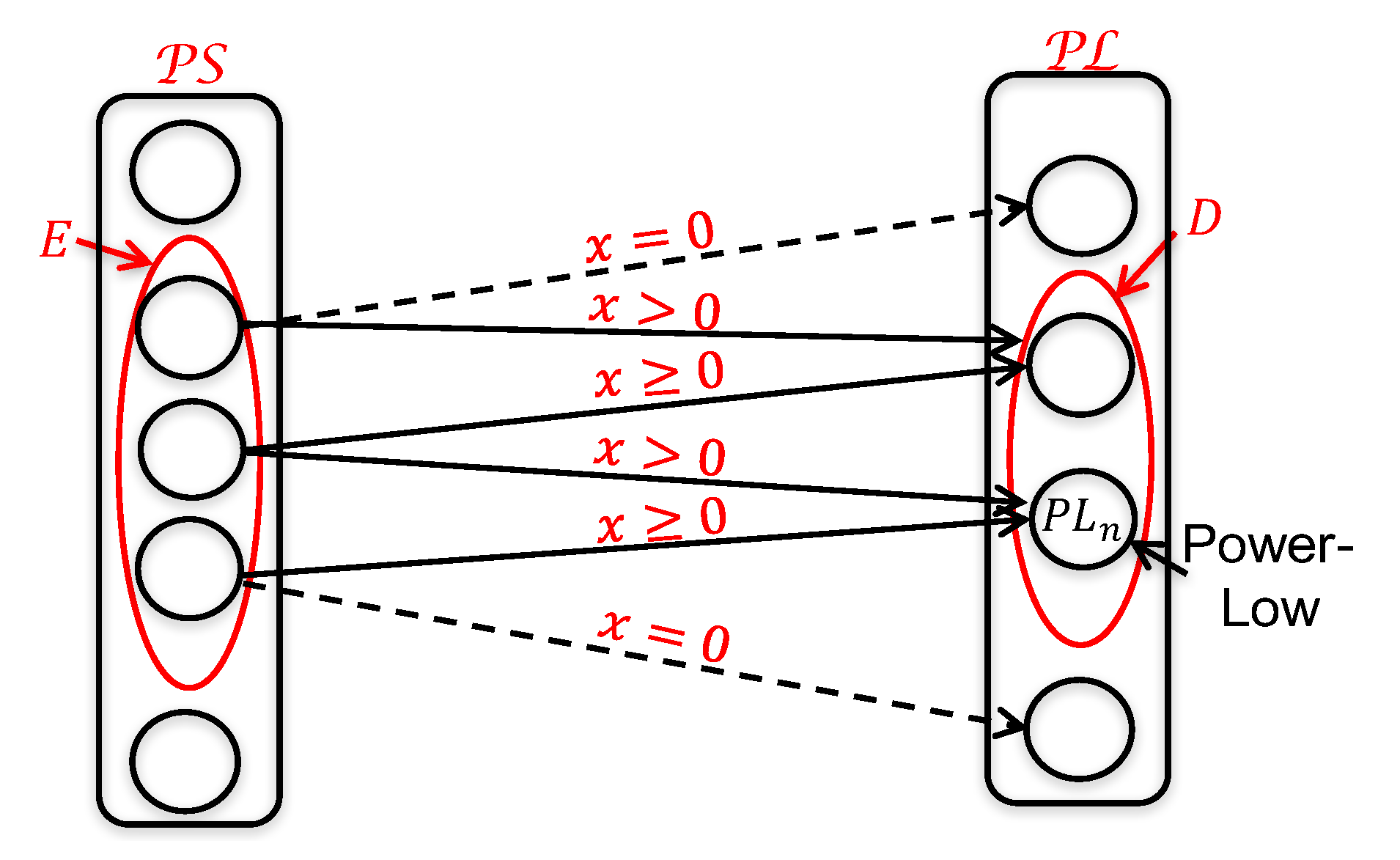
Figure 9.
Illustration of a subset E of sources and set D of loads, which can be starting nodes of alternating paths terminating at
Figure 9.
Illustration of a subset E of sources and set D of loads, which can be starting nodes of alternating paths terminating at

Figure 10.
Illustration of a subset S of power sources and set of power loads.

Figure 11.
Illustration of a subset T of power loads and set of power sources.

Figure 12.
Demonstration example for feasible solution case.

Figure 13.
Demonstration example for non-feasible solution case.


Table 1.
List of subset S of and .
| S | |||
|---|---|---|---|
| 0 | 5 | ||
| 7 | 7 | ||
| 2 | 6 | ||
| 7 | 12 | ||
| 2 | 6 | ||
| 9 | 12 | ||
| 9 | 12 |
© 2020 by the authors. Licensee MDPI, Basel, Switzerland. This article is an open access article distributed under the terms and conditions of the Creative Commons Attribution (CC BY) license (http://creativecommons.org/licenses/by/4.0/).
Share and Cite
MDPI and ACS Style
Javaid, S.; Kaneko, M.; Tan, Y. Structural Condition for Controllable Power Flow System Containing Controllable and Fluctuating Power Devices. Energies 2020, 13, 1627. https://0-doi-org.brum.beds.ac.uk/10.3390/en13071627
AMA Style
Javaid S, Kaneko M, Tan Y. Structural Condition for Controllable Power Flow System Containing Controllable and Fluctuating Power Devices. Energies. 2020; 13(7):1627. https://0-doi-org.brum.beds.ac.uk/10.3390/en13071627
Chicago/Turabian StyleJavaid, Saher, Mineo Kaneko, and Yasuo Tan. 2020. "Structural Condition for Controllable Power Flow System Containing Controllable and Fluctuating Power Devices" Energies 13, no. 7: 1627. https://0-doi-org.brum.beds.ac.uk/10.3390/en13071627
Note that from the first issue of 2016, this journal uses article numbers instead of page numbers. See further details here.