1. Introduction
As a consequence of the high increase in the installed capacity of grid-connected PV plants in recent years, it is quite difficult to plan the growing amount of energy from renewable sources fed into the grid, which is up to now non-programmable. This factor cannot be ignored any longer in the management and control of the load in the transmission network and distribution.
Moreover, considering that the distribution networks are now becoming from passive to active and that production or consumption plants [
1] are gradually becoming more and more important actors in the management of the global electrical system, it is necessary to wonder what is the reliability and accuracy level of the forecasting systems, with particular reference to wind and solar plants [
2].
In this perspective, it is easy to understand how the reliability factor of the forecast becomes a key issue in the set of rules for the identification of incentives or penalty mechanisms, in particular in finding the best mix between programmable and non-programmable sources (as defined in [
3]).
In this case, a different definition of prediction error potentially triggers a significant impact in the economy for the share of the daily energy actually produced every day in comparison with the relevant declared forecasting.
For the system management in the areas of regulation, as regards the operators of transmission networks, in addition to real-time and accurate detection of the power fed into the grid, a precise prediction of energy supply in the short and medium term is also of the utmost importance.
In recent years, the national European regulatory authorities (particularly in Italy [
4]) began to define a number of law provisions aimed at improving the prediction of the input power from renewable sources that cannot be planned, increasing gradually producers’ responsibility. In addition, several transmission networks managers will rely on the operators in the field of monitoring of photovoltaic systems for the prediction of energy generation from solar energy [
5].
In this context the need for a one-day ahead forecasting of the energy production on an hourly basis, by means of soft computer techniques starting from weather forecast provided by meteorological service, can play a fundamental role and becomes extremely useful for optimal management of the energy system. For example the same problem with different approach has been studied in [
6] where a MPC-based (Model Predictive Control) strategy is performed in real-time with accurate short-term PV power predictions.
Usually the complex nature of many practical problems involves an effective use of Artificial Neural Networks (ANNs) to solve them. ANNs are useful tools when it is necessary to understand the complex and nonlinear relationships among data, without any previous assumption concerning the nature of these correlations. The training is one of the most critical phase. In this step the weights of the neural connections have to be properly set in order to have an appropriate simulation of the performance of a PV plant. Recently, even in other application fields like for example traffic flows, hybrid evolutionary algorithms have been applied to obtain more appropriate parameter combination to achieve more accurate forecasting [
7]. In this paper the parameters of a neural network is optimized in order to reach a good and accurate output using a different kind of hybrid technique.
The ANN learning process should result in finding the weights configuration associated to the minimum output error, namely the optimized weights configuration. Usually problems are associated to an objective function to be optimized. Thus this function, called also “fitness”, cost or energy function, provides the interface between the physical problems and the optimization algorithm itself. The huge number of variables is the first difficulty when dealing with one of these optimizing issues. Secondly, there are lots of configurations with different values of the objective function that are quite similar each other and very close to the global optimum case, even if these configurations are sub-optimal. Generally finding a solution in an optimization process means to reach a balance among different and often conflicting goals; as a consequence such a search could be extremely difficult.
Among the various renewable energy sources, this study refers specifically to photovoltaic plants, without precluding the applicability of the proposed methods to other energy sources.
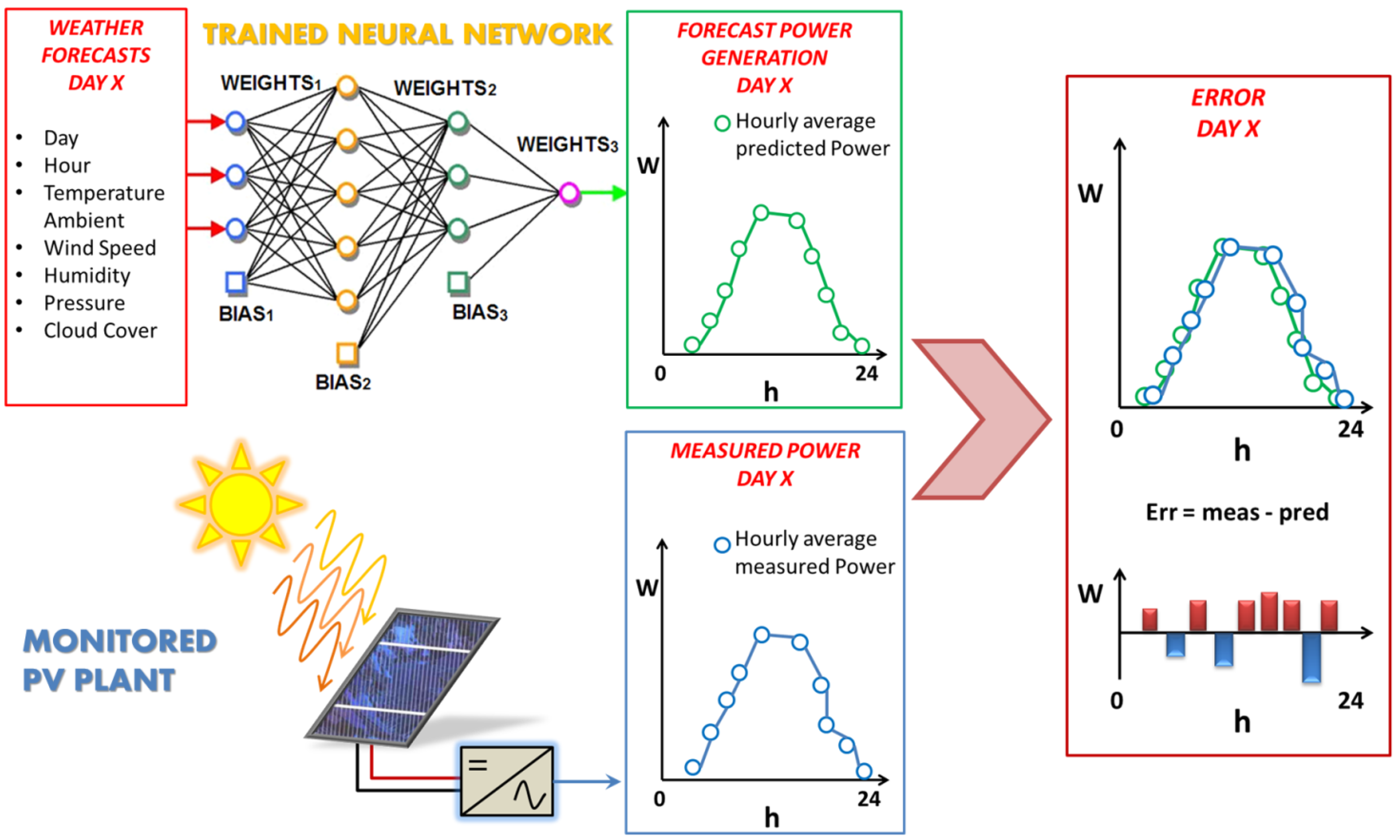
In this context the paper introduce a specific hybrid evolutionary algorithm to artificial neural networks in order to speed up the convergence when applied to ANN training phase and reduce the overall error in PV plant production forecasting applications. ANN and its training with combination of other computational intelligence (CI) techniques are nowadays very well established, nevertheless the paper does not aim to present a pure theoretical contribution, but introduces a novel application in PV power forecasting to be potentially used by power plant management operators and institutions. The whole forecasting flow is shown in
Figure 1. The next sections describe in detail implementation of such technique showing the advantage in integrating evolutionary algorithms (EAs) in ANN models.
Figure 1.
Forecasting flow process.
Figure 1.
Forecasting flow process.
2. Hybrid Evolutionary Techniques Combined with ANN
Error Back Propagation (EBP) algorithm is a well-known analytical algorithm used for neural networks training. In literature, there are several forms of back-propagation, all of them requiring different levels of computational efforts; the conventional back-propagation method is, however, the one based on the gradient descent algorithm. The strong dependence upon the starting hypothesis that severely affects the result is one of the drawbacks of this method. A bad choice of the starting point may result in the possibility to get stuck in a local minimum and consequently to find a solution that is not the best one. Besides, most of the typical requiring optimization problems often have non-differentiable or/and discontinuous regions in the solution domain therefore some difficulties interfere in the application of these traditional methods based on derivatives calculations. These aspects are often overcome by evolutionary methods. The most effective evolutionary algorithm developed until now is Genetic Algorithm (GA), which is now quite familiar to the engineering community and widely used ([
8,
9] and references therein). Genetic algorithms are very efficient at exploring the entire search space, but are relatively poor in finding the precise local optimal solution in the convergence region. Some additional operators can be introduced for GA in order to get a better predictive power of ANNs selecting an optimal combination of input variables. Moreover, in recent years also the Particle Swarm Optimization (PSO) algorithm is gaining increasing attention for the integration in the training phase of ANNs [
10,
11].
Recently hybrid evolutionary techniques have been developed in order to combine the best properties of classical GA and PSO to overcome the problem of premature convergence. Some comparisons of the performances of them [
12] emphasize the reliability and convergence speed of both methods, but still keep them separate. These procedures show a marked application driven characteristic for any respective technique: PSO seems to have faster convergence in the first runs, but often it is outperformed by GA for long simulations, when the last one finds better solutions. Some attempts to exploit the qualities of the two algorithms have been done in the last ten years with a kind of integration of the two strategies [
13], but the authors aimed to reach a stronger co-operation of the two techniques stressing its hybrid nature and maintaining the GA and PSO integration for the entire run of the algorithm. Thus in the last years the authors have developed an innovative hybrid strategy called GSO, Genetical Swarm Optimization, which proved to improve traditional evolutionary mechanisms for a wide range of applications by means of an effective combination of natural selection and knowledge sharing. In particular, in [
14], some comparisons of GSO and classical methods performances were presented, emphasizing the reliability and convergence speed of the first one and applying it to different case studies.
The basic concepts of GSO have been presented in [
15]: in every iteration, the population is randomly divided into two parts that are evolved with GA and PSO techniques respectively. Then the fitness of the newly generated individuals is evaluated and they are recombined in the updated population, which is again divided into two parts in the next iteration for the next run of genetic or particle swarm operators. The population update concept can be easily understood thinking that a part of the individuals is substituted by new generated ones by means of GA, while the remaining are the same of the previous generation but moved on the solution space by PSO. The driving parameter of GSO algorithm is the so called hybridization coefficient (
); it expresses the percentage of population that in each iteration is evolved with GA with respect of PSO technique. GSO has been tested on problem of different dimensions: while for a small number of unknowns GSO performance is similar to GA and PSO ones, if the size of the problem increases, GSO behavior improves and outperforms GA and PSO during iterations. Moreover, the best
value found in that preliminary study does not depend on the dimension of the problem, as it has been reported also in [
14]. Furthermore, the obtained best
value between 0.2 and 0.3 means that for a big-sized problem, the basic PSO can be strongly improved by adding a small percentage of genetic operators on the population. In further studies a convenient value was found to be in the same range for several fitness functions, but the authors extended the class of GSO algorithms by considering several variation rules for
, in order to explore different hybridization strategies for the GSO algorithm and to compare new approaches with others already present in literature. The full set of hybridization rules considered by the authors is also reported in [
16].
In [
15] the authors introduced new rules for varying the
value during the run, to combine more efficiently the properties of GA and PSO, in order to have a general procedure. In fact for engineering optimization problems the best mix of GA and PSO operators cannot be known a priori. In particular there are situations where a fixed
is the right choice, and others where a variable
during the run is better. This means that also the “amount” of hybridization plays a role in affecting the performances of this procedure. Therefore the authors chose to let the procedure adjust the
value by itself during the iterations, according to a predefined set of rules defining two different approached defined as dynamical and self-adapting, where the rule implemented comes in part from the very simple and reliable swarm techniques.
The overall results reported by the authors in cited papers show that, although the static GSO is generally the faster and more robust strategy in order to optimize multi-modal functions, a self-adaptive approach is a suitable and reliable solution especially when the proper value is not known for a specific problem. The overall results reported by the authors in cited papers show that GSO is a good candidate to be used in classical neural networks to replace training procedure as for example the common EBP (Error Back Propagation).
In this work a dynamic GSO was combined with a classical EBP in order to improve the speed of convergence of the neural network training phase and, at the same time, to improve the performance of the predictive system. In [
17] the authors started to apply hybrid evolutionary learning algorithm to increase the accuracy of the daily forecast finding the best neural weights configuration. Here a similar mixed approach is used to optimize the neural weights in a more complex predictive model where the one-day ahead production estimation is performed on a hourly base [
18].
Before showing how such a technique has been applied to a specific real case study, in the next section we will discuss some error definitions in order to identify the most appropriate formula that better describes the gap between declared and really produced energy in the context of future incentives or penalty mechanisms. (e.g., according to Italian regulation Authority [
4]).
3. Error Definitions
The application of the technique described in the previous paragraph to the problem of PV production forecasting requires a proper and shared definition of the error estimation with the aim to assess the amount of the daily produced and declared energy. In order to correctly define the accuracy of the prediction and the relative error, it is necessary to analyze different definitions of error. The starting point reference is the hourly error
, defined as the difference between the average power produced in the hour
and the given prediction
[
4] provided by the neural model:
From this basic definition, other definitions can be introduced:
Absolute hourly error , which is the absolute value of the previous definition (
can give both positive and negative values):
Daily error , given by the summation extended to 24 hours
time error:
Daily absolute error , given by the summation extended to 24 hours of the Absolute Hourly Error:
Time error percentage based on the rated power of the photovoltaic (
):
Time error percentage based on the hourly output expected power (
):
Following Italian regulation authority, the penalties concerning the transitional period of the year 2013 will be calculated on its basis.
Daily time error percentage, based on the hourly output expected power (
):
Moreover some considerations on the accuracy of measurements related to the plant available instrumentation affecting the input raw datasets and dispersion evaluation on these data from the expected values should be considered in a validation phase before starting the ANN training process itself.
4. Case Study
After a trial campaign, the network architecture that has provided better results presents two hidden layers. In particular, the number of neurons in the input layer is 7, as shown in
Figure 2, which describes the meteorological parameters provided from the weather forecast service.
Figure 2.
Simplified view of the implemented feed-forward ANN with details on input, output, and hidden layers.
Figure 2.
Simplified view of the implemented feed-forward ANN with details on input, output, and hidden layers.
This network structure is less complex than the one proposed by another comparative study on power forecasting methods in PV plants [
18], where the authors used neural networks with hidden layers and a number of neurons in a higher range (from 11 to 15); in our work in fact we use two hidden layers with, respectively, 9 and 7 neurons, while the output layer is composed by 1 neuron. The authors, in fact, performed preliminary simulations for different photovoltaic power plants in order to test their method at various scale, with different productive capacities, to make this procedure more general [
19].
Different time horizons can be considered in power forecasting: short term (day and several days), medium term (week and several weeks), long term (year and several years), and forecasts for different lead time can be used for different aims. Here, we chose a very short term time base for this specific application, giving one-day ahead forecasting on an hourly basis in accordance with [
20], since this is the typical resolution requested by power plant operators. In this work the neural network optimized by GSO exhibit good predictive performances in all the operative conditions, in a complete sunny day, a partly cloudy one and even a plant maintenance day. Here a combination of GSO and EBP was used for the hybrid learning process of the artificial neural network, as described in [
19], and weights values of the ANN were changed to reach the minimum error in the network output in a faster way compared with standard EBP alone. In literature other evolutionary procedures as standard PSO and GA were compared with the classical EBP in order to perform a comparison in terms of convergence rate and final obtained result (e.g., [
21]), but GSO has already proven to outperform both GA and PSO [
14].
In particular, here the GSO-based training phase is first conducted for 9000 iterations (with a population of 50 individuals) over a period of one year, to process a global search of weights values; the EBP training is then used for additional 5000 iterations to refine the optimal weights configuration. To show the effectiveness of this hybrid approach, results are then compared with those obtained by running a standard EBP learning for a comparable amount of computational time, i.e., for 500,000 iterations.
5. Data Validation and Training
The neural network has to be calibrated with previously collected data on the energy production, along with the weather forecasts, for a sufficiently long time (a full calendar year would be an appropriate reference). On the basis of the actual measurements, the error is calculated after applying different criteria for defining it as discussed in the next section. The previously described method has been applied to the production forecast of a PV test plant managed by the Department of Energy of Politecnico di Milano.
The considered input parameters are the following physical quantities provided by the weather forecast service:
In particular, since we cannot have a forecast of the temperature for each specific module in a plant, we take into account factors that are correlated with that value, i.e., the environmental temperature, wind speed and humidity.
The average hourly power () forecast in the “h” hour is then calculated as the output value for the next day.
This value is compared with the following meteorological and physical quantities:
is the average hourly power produced by the PV plant in the “h” hour (W);
is the Global Irradiance on the horizontal plan (W/m);
is the Global Irradiance on the tilted plan (W/m
) (as defined in [
22]);
is the percentage of the cloud coverage (%) (as defined in [
23]).
The irradiance data are compared with the theoretical values on the tilted plan
Irr,Th.Tilt assessed by a deterministic algorithm on the basis of the geographical coordinates with the aim to validate the forecast data. The input data have been validated in order to verify their true significance or to provide the proper training to the network. For example all irradiation samples by night were omitted to exclude a high rate of forecasting elements that could highly affect the resulting error (irradiance forecasts during the night are zero). All the missing data have been excluded not contributing to the forecast. Starting from the comparison between the actual produced power and the predicted one, it is calculated for each day:
the hourly error ;
the error percentage, based on the rated power ;
the error percentage on the hourly power forecast ;
the daily error percentage based on the hourly power forecast .
6. Results and Discussion
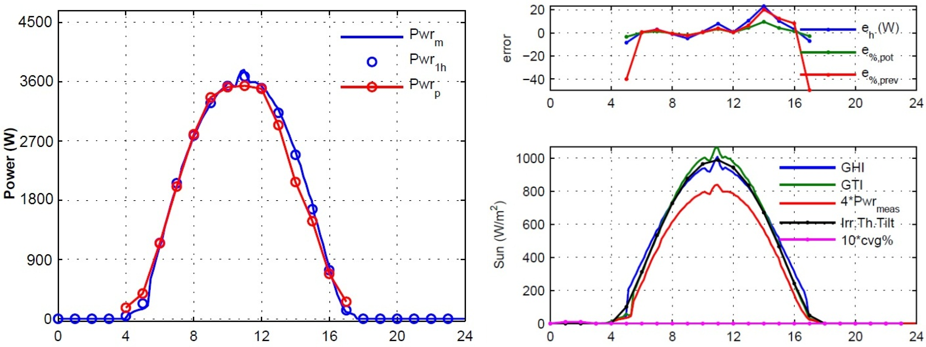
The described forecasting technique has been applied over a one year production period. Two days are displayed hereunder, the first one showing good weather conditions (
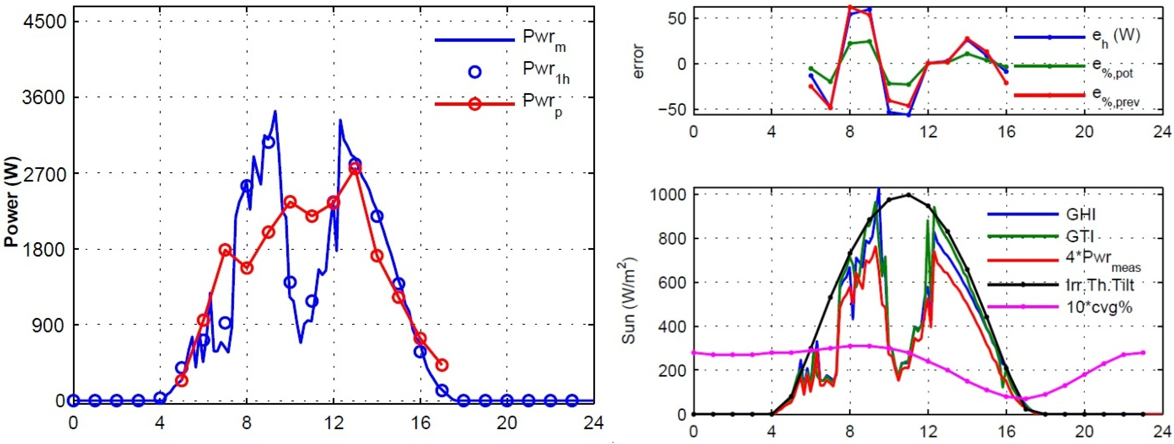
Figure 3), the second day showing bad ones (
Figure 4).
Table 1 reports detailed energy production and error calculation for the two sample days.
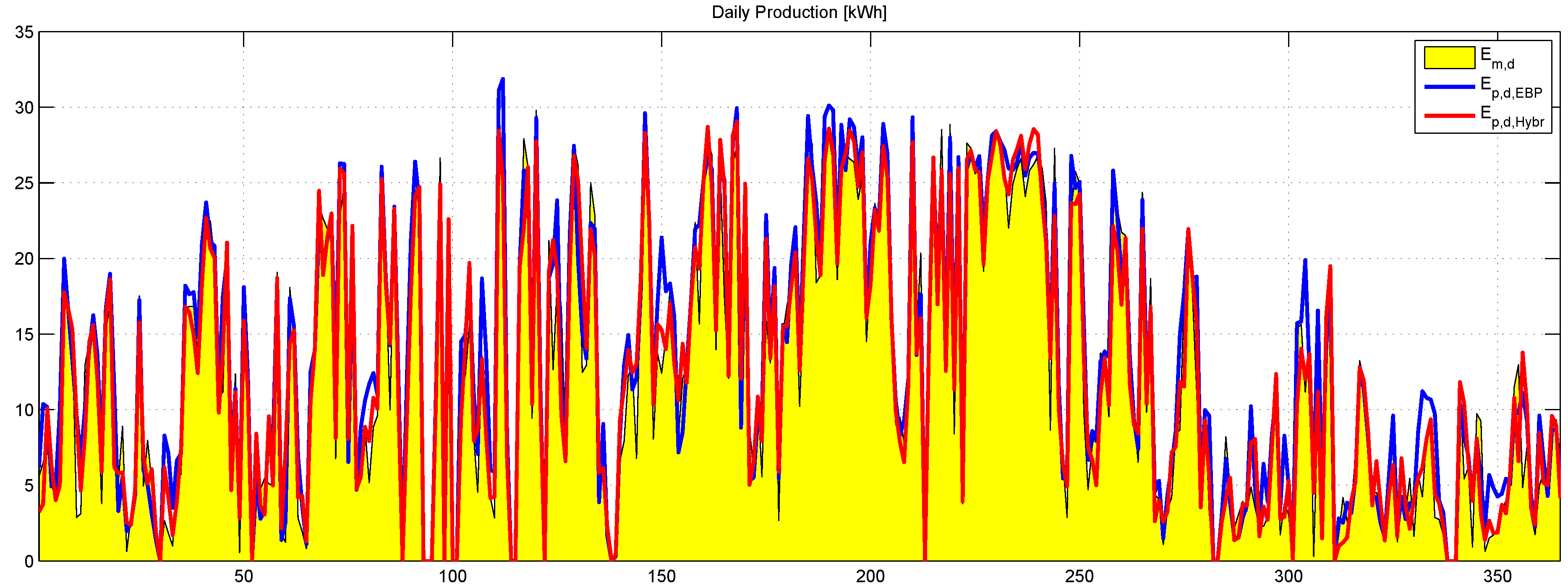
Figure 5 and
Figure 6 respectively report the comparison between the forecast results and errors obtained by the hybrid training (GSO + EBP) and the standard EBP alone, showing an improvement of performances using the hybrid approach for the same computational time. In particular, these results are summarized in
Table 2, where the two training approaches are compared considering some of the error definitions previously introduced in
Section 3.
Figure 3.
Daily detail of the curves of radiation (theoretical, forecast and actual) with the calculation of the error values during a clear sky day.
Figure 3.
Daily detail of the curves of radiation (theoretical, forecast and actual) with the calculation of the error values during a clear sky day.
Figure 4.
Daily detail of the curves of radiation (theoretical, forecast and actual) with the calculation of the error values during day with bad weather conditions.
Figure 4.
Daily detail of the curves of radiation (theoretical, forecast and actual) with the calculation of the error values during day with bad weather conditions.
Figure 5.
Daily produced and predicted energy comparison.
Figure 5.
Daily produced and predicted energy comparison.
Figure 6.
Daily absolute error comparison.
Figure 6.
Daily absolute error comparison.
Table 1.
Production data and error calculation for two-day examples.
Table 1.
Production data and error calculation for two-day examples.
| Physical quantities | Clear sky day | Cloudy day |
|---|
| Daily Production | 28.37 kWh | 19.16 kWh |
| Daily Forecast | 27.68 kWh | 19.65 kWh |
| Daily Error | 684 kWh | −491 kWh |
| Daily Error percentage on the base of the daily production | 2.41% | −2.56% |
| Daily Error absolute | 2.29 kWh | 5.96 kWh |
| Daily Error percentage on the base of hourly forecast power | 8.08% | 30.31% |
Table 2.
Main production data and error calculation with reference to the entire period.
Table 2.
Main production data and error calculation with reference to the entire period.
| Forecast error definition | | EBP | Hybrid (GSO + EBP) | |
|---|
| Nr. Samples | | 2879 | 2879 | h |
| Average Hourly Abs. Error | | 0.338 | 0.317 | kW |
| Yearly Total: | | | | |
| Overall Production | | 4512.3 | 4512.3 | kWh |
| Overall Forecast | | 4852.6 | 4562.4 | kWh |
| Overall Yearly Error | | −340.3 | −50.12 | kWh |
| Error abs. tot | | 973.2 | 912.98 | kWh |
| Error abs.% tot | | 20.06% | 20.01% | |
| Daily Averages: | | | | |
| Average Daily Production | | 12.36 | 12.36 | kWh |
| Average Daily Forecasting | | 13.29 | 12.50 | kWh |
| Average Daily Error | | −0.932 | −0.137 | kWh |
| Average Daily Abs. Error | | 2.666 | 2.501 | kWh |
The developed model allows an accurate prediction generally for clear days as well as for permanently covered days. However, as shown in
Figure 4, there was a lower precision in the days characterized by a strong and rapid variability. In fact, since data provided by the weather service are on hourly basis, we lose information that is particularly important in days with highly variable cloudy conditions. In particular, this problem could be also due to the slowness of
forecast with respect to the actual fluctuations of the other meteorological parameters: probably this index is averaged over several hours and, therefore, it is unable to represent accurately the real variability of the actual cloudy coverage.
Additional considerations can also be made with regard to the formulation of the forecasting error. For example the error percentage on the hourly power forecast is always high in correspondence of values of low solar radiation. This event occurs both during cloudy days and during sunrise and sunset of any day. As in these periods of time the power generation is relatively small, the forecasting error should not be counted in the same way as the forecasting error calculated during the hours with high level of solar radiation. In these conditions, the authors suggest a threshold of solar radiation under which the data have not to be considered. Besides, in this error definition, the measured power data should be adopted instead of the forecast power ones.
7. Conclusions
Due to the increase of renewable energy penetration in the electric grid, it is quite important to estimate the amount of energy from such non-programmable sources.
In this paper a novel hybrid evolutionary approach is used for training artificial neural network in order to achieve more accurate forecasting of photovoltaic systems based on weather forecast as input data. Moreover, analyzing all test results obtained by comparing different definitions suggested for the forecasting error, a sensible reduction of the error itself can be achieved by increasing the time range of observation and of course the quality and resolution of the data provided from the local weather forecast service.
The developed model allows both better predictions and potential novel applications in PV power plant management operations.


