
Carbon Auction Revenue and Market Power: An Experimental Analysis

John Glenn College of Public Affairs, The Ohio State University, 1810 College Rd, Columbus, OH 43210, USA
Energies 2016, 9(11), 897; https://0-doi-org.brum.beds.ac.uk/10.3390/en9110897
Submission received: 15 August 2016
/
Revised: 29 September 2016
/
Accepted: 13 October 2016
/
Published: 1 November 2016
(This article belongs to the Special Issue Contemporary Sustainable Energy Paradigms and the Multifunctional Economy)
Abstract
:State and regional governments in the U.S. and abroad are looking to market-based approaches to mitigating greenhouse gas emissions from the electric sector, and in the U.S. as a compliance approach to meeting the aggressive targets of the Environmental Protection Agency (EPA)’s Clean Power Plan. Auction-based approaches, like those used in the Northeast U.S. and California, are both recommended strategies under the Plan and attractive to state governments because they can generate significant revenue from the sale of emissions permits. However, given the nature of imperfect competition in existing electricity markets, particularly at the state and regional level, the issue of market power is a concern at the forefront. This paper provides the results from a controlled laboratory experiment of an auction-based emissions market in the electricity sector. The results show that government revenue from auctioning emissions permits is substantially lower when market concentration is only moderately increased. The results hold significant implications for states and other subnational governments that have high revenue expectations from the auctioning of emissions permits.
Keywords:
carbon auctions; cap-and-trade; market power; government revenue; climate change; Clean Power Plan; Clean Air ActJEL Classifications:
C90; D43; D44; Q40; Q541. Introduction
Cap-and-trade programs have provided an economically efficient approach to environmental policy throughout the past three decades [1,2,3,4]. More recently, the cap-and-trade approach (carbon markets) has been applied to mitigate greenhouse gas emissions at the international, national, state, regional and municipal levels in the E.U., U.S., China, New Zealand, Canada, South Korea and Japan [5]. In the U.S., there are two operating regional carbon markets—the Regional Greenhouse Gas Initiative (RGGI) in the Northeast, and the California AB32 market. Last year, the Environmental Protection Agency put forth the Clean Power Plan, a regulatory mandate under the Clean Air Act (Section 111d) that requires states to substantially reduce greenhouse gas emissions from the electricity generation sector. The plan outlines a number of compliance strategies for states, the first among which is a recommendation to utilize a carbon market, or to join an existing regional carbon market in either California or RGGI.
To state legislatures, revenue from the sale of carbon permits appears, on the surface, to be an attractive aspect of carbon markets as a compliance strategy moving forward. However, the issue of market power, which has been identified in both the scholarly literature and in practice, in both electricity markets [6,7,8,9,10,11,12,13] and cap-and-trade markets [14,15,16,17,18,19,20,21,22,23,24], may have a noticeable effect on states’ ability to raise revenue under carbon markets modeled after RGGI or California. Market power is exercised in carbon auctions (detailed below) as strategic demand reduction (i.e., a strategic bidding approach) to suppress permit prices. It is exercised in electricity markets as strategic supply reduction to create artificial shortages and inflate the selling price of electricity, either through physical or virtual bidding. Both the California and RGGI markets are state-level cap-and-trade programs in which the electricity generation sector is the predominant sector of compliance [25], and in which nearly 100 percent of the permits are allocated using auctions. Simply put, auctions are almost exclusively used to allocate emissions permits among firms in a thin product market with a well-documented history of market power and market manipulation.
Recent evidence suggests that carbon markets and electricity markets operate with some interdependency. That is, energy-emissions market linkages can be utilized by dominant firms to inflate the selling price of electricity [26,27,28,29,30]. And, recent experimental evidence has shown that strategic supply withholding in the energy market is not only profitable in the energy market alone, but is also an implicit demand reduction in the carbon market [31]. That is, withholding energy from the market not only raises the sale price of energy, but also reduces the market price of carbon permits in auction-based cap-and-trade programs, thus reducing the costs of compliance with the emissions program.
Given this dynamic, states (or other subnational jurisdictions) that are attempting to construct cap-and-trade programs in their jurisdictions may be unaware of the degree to which a divergence exists between expected revenue and revenue under imperfect competition. This paper provides evidence from a series of controlled laboratory experiments of a joint carbon-energy market based upon the RGGI market design. The paper tests three formalized hypotheses and provides evidence that state governments can expect substantially less revenue from the auctioning of carbon permits when firms hold modest market power (an increase in the Herfindahl–Hirschman Index (HHI) from 1000 to 2000). The next section of the paper provides a brief background on supply side and demand side influences on government revenue in auction-based carbon markets that motivates the experimental approach undertaken in this research. Section 3 provides details on the experimental design, and Section 4 provides the formalized hypotheses and data. Section 5 provides the experimental results. And, Section 6 concludes with implications for state governments in the U.S. (and foreign governments) in considering carbon markets as a policy mechanism for reducing greenhouse gas emissions or complying with the new Clean Air Act regulations under the Clean Power Plan.
2. Background
Because the effect of imperfect competition on government revenue is the focus of this research, it is important to note that the revenue that governments receive from the sale (via auctioning) of carbon permits is affected by both supply side and demand side effects. Ex post assessments of the effect of market power on government revenue cannot directly observe variance in market composition or energy market dynamics; however, these effects can be explicitly tested in a controlled lab experiment, as provided here. The RGGI market is the predominant focus of this background given that there is substantially less operational history in the California markets to draw upon, given that California and RGGI are both auction-based markets, given that RGGI is mentioned in the Clean Power Plan first and numerous times, given that the European Union Emissions Trading Scheme (ETS) markets do not yet utilize auctions (but will in the future), and specifically given that states are predominantly looking to U.S. markets to inform their compliance approaches under the Clean Air Act.
2.1. Supply-Side Effects
The regulators’ decision regarding the quantity of emissions allowances issued is subject to both a scientific as well as a political process. Regulators aiming to maximize social welfare will set the quantity of emissions allowances at the socially-efficient level, determined by an external technical and scientific process, which is outside the scope of this analysis. Regulators aiming to maximize government revenue from the sale of emissions allowance may ultimately set the supply of emissions allowances at a level that is substantially different from the socially-efficient one. The law of supply would simply suggest that an over-allocation of emissions allowances relative to a generally fixed demand for allowances (in the short-run) would lead to a decline in the price of emissions allowances. This would suggest that the revenue from the sale of those emissions allowances would also decrease as allowance allocation exceeds demand. Therefore, the quantity of emissions allowances allocated by the regulator plays a significant role in the revenue generated.
In the New England carbon market (RGGI), a majority of state governments participating in the multi-state market, generously over-allocated the supply of emissions allowances they sold into the regional nine-state market. The New England market functions as a regional market in which each state sets its own allowance budget to be auctioned in the central regional auction. Allowances are perfectly substitutable, in that allowances issued by a state can be surrendered for compliance in any participating state. Naturally, a collective action problem arose when each state, in their attempt to maximize revenue to their state from the sale of allowances, collectively inflated the aggregate supply of allowances.
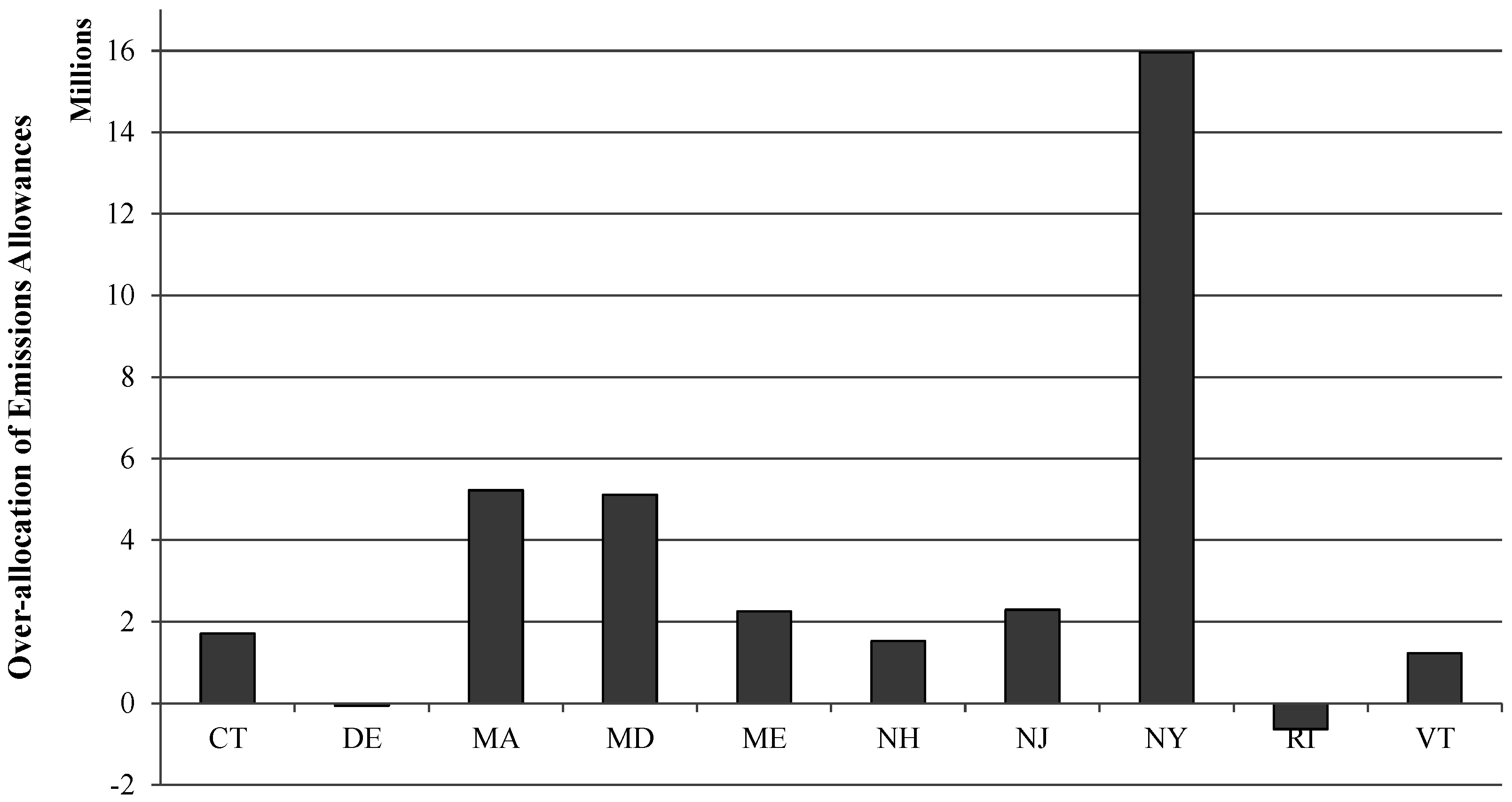
Figure 1 and Figure 2 provide the state-by-state over-allocation of emissions allowances in the New England carbon market in millions of tons of carbon dioxide equivalents (CO2e). To assist state governments in making their allowance budget allocations, an annual carbon inventory was taken, dating from 2000 until the program’s inception in 2008. Figure 1 provides the over-allocation of allowances from the most recent year’s inventory (2008) and Figure 2 provides the over-allocation of allowances from the 9-year average from 2000 until 2008. In total, only Delaware and Rhode Island issued allowances for a quantity of carbon emissions below their historic emissions levels. It should be noted that the ETS markets are also substantially over-allocated, but are not auction-based markets yet.
It is commonly thought that a government will aim to maximize social welfare rather than revenue. Inflating the “cap” of allowances beyond emissions levels negates the intent of the program altogether (i.e., permits are sold but emissions are not reduced). At the same time, government revenue was severely influenced by the supply-side reaction that occurred. Carbon auction prices stayed almost consistently at the auction price minimum, an auction reserve price that ranged from $1.86 to $1.98.
After four years of operation, New England states announced a 45 percent, across the board reduction in the supply of emissions allowances. Since then, auction prices have increased moderately above the reserve price. During initial program development, economic analyses provided price estimates based on the initial allowance allocation (prior to the 45 percent cut) of between $7 and $14 [32], and some external analysts predicted higher prices. The past few quarterly auctions in RGGI, following the nearly fifty percent cut in the supply of permits, have seen auction clearing prices in the neighborhood of $4.00 to $5.00 per ton. None of the prior analyses explicitly tested for the effect of imperfect competition.
2.2. Demand-Side Effects
There are two main demand-side effects that influence government revenue from emissions allowance auctions. First, exogenous effects such as fluctuations in weather and economic growth can substantially influence the long-term demand for emissions permits [16]. Second, market composition and behavioral influences stemming from market failures, such as market power, can influence government revenue both in the long and short run. The latter of which is the subject of the analysis presented here.
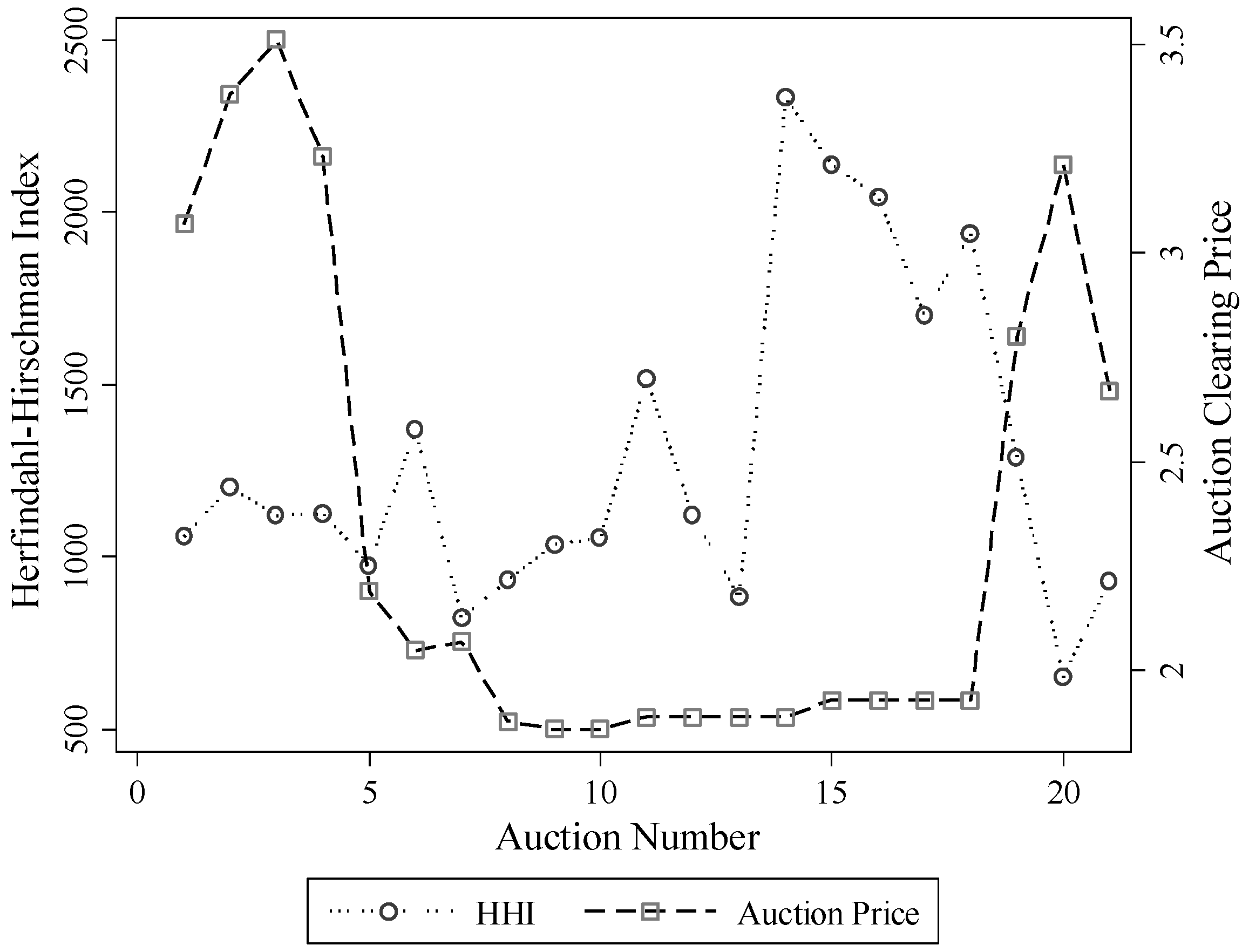
Figure 3 provides a measure of market concentration in the New England carbon market, dating back to the program’s inception in 2008. The HHI of market participants is provided, and ranges from approximately 1000 to 2000. Figure 3 also provides some descriptive evidence that auction price is inversely related to market concentration, although, that is not formally tested here. That is in the expected direction; as the market becomes more oligopolistic, dominant firms are able to utilize their price influence to suppress the price of emissions allowances [15,17,23,33,34,35]. Dormady [17] provides the results of repeated Monte Carlo simulations on the influence of market power through strategic demand reduction in uniform-price auctions. Consistent with demand reduction behavior, firms with market power bid strategically to lower the auction clearing price and acquire allowances at a lower price than in a competitive price-taking market.
Given this, carbon auction revenues can be influenced by a variety of factors, both endogenous and exogenous to the market itself. A controlled laboratory experiment allows us to provide a set of controlled parameters to assess the impact of market composition as an independent influence.
3. Experiment Design
3.1. Experimental Setup
The experimental design simulates a stylized carbon market with inter-temporal dynamics. Although sufficient heterogeneity in market design exists across programs globally, this experiment is intended to provide a stylized market based primarily on the RGGI auctions (and the California design by extension) to test the effect of market concentration on revenue in a carbon market with auction-based allocation.
In this experiment, subjects participate in the electricity market and the carbon market simultaneously. There are two treatments within this experiment, a control treatment where all firms have equivalent price influence and market composition, and a market power treatment. The market power treatment includes oligopolists among firms with less price influence, referred to as “fringe” firms, and consistent with Hahn [24]. The energy market is designed to simulate an auction-based wholesale procurement market, such as would occur under an Independent Systems Operator (ISO) or Regional Transmission Organization (RTO) in a deregulated electricity market. In the carbon market, subjects compete in auctions to acquire emissions permits associated with the energy they have produced in the energy market. Allowances (permits or credits) are required for purposes of compliance, based upon the amount of electricity they sold into the auction (i.e., quantity produced).
The design includes additional features consistent with operating markets. These include stochastic energy demand, heterogeneous supply portfolios, inter-temporal dynamics, a declining emissions cap across time, resale arbitrage, heterogeneous budgets, and collusion among dominant firms. The specifics of the design are detailed in the next sections.
3.2. Auction Format
Both the energy market and the carbon market are uniform-price sealed-bid auctions. This format is consistent with operating markets in California and the Western Climate Initiative (WCI), the RGGI, and most operating deregulated electricity markets [36]. The uniform price auction allows for a single bidding phase in which bidders submit both a price and a quantity bid, that is rank-ordered by price, and quantities are awarded to winning bidders in the order of ranked-bid price. Non-discriminatory auction formats require winning bidders to pay the uniform (or common) auction clearing price for all winning bids, rather than the price submitted by the bidder. In this experiment, bids are ranked from highest to lowest for the sale of carbon allowances, and from lowest to highest for the sale of electricity. The decision rule utilized sets the uniform price as the lowest winning bid [37]. Krishna [38] and Dormady [17] provide useful models of the uniform-price sealed bid auction, the latter of which provides a useful matrix-based approach.
3.3. Generation Assets (Energy Portfolios)
Treatments included two types of generation assets, thus allowing for heterogeneity in aggregate production. Some generation assets were low cost (i.e., low marginal cost of production) and some were high marginal cost assets. The production cost of a low cost asset was $1 experimental, and the production cost of a high cost asset was $2 experimental. The total market available supply of energy was 20 units. The portfolio of power was evenly divided between low and high marginal cost assets, with the aggregate energy portfolio consisting of ten units of available supply from each generation asset type (i.e., 10 coal and 10 natural gas).
3.4. Energy Demand
Just as in operating energy markets, the demand for energy is stochastic and exogenous, varying with changes in weather and climatological conditions as well as supply conditions [16]. The demand for energy in this experiment, therefore, is set exogenously and stochastically. Three levels of demand were simulated; low demand, intermediate demand and high (peak) energy demand. Under low energy demand, only 10 of the 20 generators were called upon to supply energy. Under intermediate energy demand, 15 units were called, and under peak demand, all 20 units were called. The demand was set exogenously and drawn each period from a uniform distribution.
3.5. Inter-Temporal Dynamics
In each treatment of the experiment, inter-temporal dynamics were simulated by including two bidding rounds for each market simulation. Subjects bid in the energy market to sell their supply of energy competitively in both rounds, and subjects also bid in both rounds to acquire emissions allowances. The demand for energy was equal in both rounds. The supply of emissions allowances was 20 in the first round, and 15 in the second. That is, to simulate a declining emissions cap across time, 25 percent fewer allowances were auctioned in the second round, that is . This is consistent with quarterly auctions in operating carbon markets with annual compliance periods.
The emissions market also includes resale dynamics. Ceteris paribus, as the supply of emissions allowances declines with a tightening emissions cap across time, the price of emissions allowances is expected to increase [3,39]. Subjects in the experiment were permitted to resell emissions allowances acquired in the first round, into the tighter second round. Subjects were paid the uniform auction clearing price for each emissions allowances that they sold in the second round auction [40].
The supply of emissions allowances in the second round also included any emissions allowances that were unsold from the first round. The market also instituted the rule of public priority, in which allowances auctioned by the regulator were sold before allowances posted to the auction in the second round for resale. In other words, unless all of the government’s emissions allowances were sold first, market participants could not sell allowances. This is consistent with operating emissions markets that prioritize public revenue from the sale of allowances.
Another key design feature of Coasian markets is the non-compliance penalty that is enforced by the regulator. This is typically operationalized as a penalty for acquiring an insufficient quantity of emissions allowances during a pre-specified compliance period (usually annual). In this experiment, a non-compliance penalty of $5 experimental was imposed per missing, or short allowance. For example, a producer that supplied four units of energy and was required to surrender four emissions allowances at the end of the market simulation, but only surrendered two allowances, would incur a penalty of $10 experimental ($5 times two short allowances).
Implicit within this experimental design is the concept of banking of emissions allowances. Banking is the principle by which firms can inter-temporally optimize their abatement and allowance acquisition in order to maximize firm-level profit [41]. Just as in operating markets, in this experiment the non-compliance penalty only came at the end of the compliance period (i.e., round 2) and thus, subjects could freely determine their own temporal compliance strategy.
3.6. Market Composition
Each treatment of the experiment included ten subjects. In the control treatment without market power, each subject controlled 10 percent of the supply (HHI = 1000) [42]. In the treatment with market power, two subjects were oligopolists with 30 percent of the supply each, and the remaining eight subjects each controlled 5 percent of the supply (HHI = 2000).
In the control treatment, each subject had a supply portfolio of two generation assets. These included one high cost and one low cost asset for each subject. Each subject was also given an opening bank account, or budget, of $20 experimental to utilize for the purchase of emissions allowances. In the market power treatment, each oligopolist had a supply portfolio of three low cost generation assets and three high cost generation assets. Oligopolists had an opening budget of $60 experimental. Fringe bidders each had one generation asset, and were randomly assigned ownership of either a low or a high marginal cost generation asset. Fringe subjects had an opening bank account of $10 experimental. As such, each bidder had an opening bank account of $10 experimental for each generation asset they owned in a bidding period.
In operating energy markets, bidders are often limited by a bid cap. These bid caps are often put in place to limit the extent of price influence. This cap operates as a bid price ceiling on the marginal price of supply. This experiment included a bid cap of $10 experimental per energy unit sold.
3.7. Communication Medium
The two oligopolists were permitted to use a chat communication tool to communicate with one another during the bidding phase of the experiment. This communication tool was only viewable to the two subjects who were oligopolists during the period of the experiment in which they were assigned to the oligopolist type. This feature was put in place so that collusion between oligopolists could occur.
3.8. Experiment Operation
To avoid framing effects, market-specific terminology was removed from the experiment to decontextualize the experiment. High and low cost generation assets were referred to as “Product X” and “Product Y”, respectively. Emissions allowances were called “licenses” instead of “allowances” or “permits”.
Session duration was 3 h. The first hour consisted of a 60 min instructional MP4 video that instructed subjects on the rules of the experiment, client software, and a very brief set of example scenarios to illustrate profit calculation and resale in the two-stage game. Experiment videos were recorded using Jing Pro [43]. The software environment utilized for this analysis was the Zurich Toolbox for Readymade Economics Experiments (ZTREE) and its companion client application Z-Leaf [44].
The experiments were conducted at the University of Southern California Law School (Los Angeles, CA, USA). Subjects consisted of graduate and undergraduate students across all university majors. Subjects were randomly assigned to experimental sessions. To ensure further randomization, treatments were assigned randomly to sessions. In the treatment sessions, subjects were also assigned randomly to bidder types each period, as mentioned above. Within each experimental session, approximately 30 two-round energy-emissions market simulations were conducted.
Subjects each received a $10 show up payment. Session payments had a 0.1 conversion rate. This means that in addition to the show up payment, subjects received ten cents for every dollar they earned during the session. Subjects had an earnings cap of $60. Another constraint was put in place to guard against subject losses. In the event subjects ever incurred losses in any bidding period, the software would simply record their earnings as $0 experimental.
3.9. Government Revenue
Government revenue from the sale of emissions allowances in a carbon auction is a function of both price and quantity across all auctions within the compliance period. Ceteris paribus, the more emissions allowances sold in a carbon auction, the greater the revenue the auction will yield for the government. Similarly, the greater the price of allowances sold in a carbon auction, the greater the revenue the auction will yield for the government. Government revenue in a given auction at time t is given by and is therefore a function of the auction-clearing price and quantity of emissions allowances sold in that auction, given by:
In markets with multiple (e.g., quarterly) auctions within a compliance period (e.g., annual), government annual revenue is the sum of auction revenues across those auctions. In this experiment, a simplification was made such that there were two carbon auctions held in a single compliance period, and thus government revenue in the compliance period, denoted by R, is the simple sum of revenue across round 1 and 2, or and , respectively, as given by:
The nature of compliance periods is such that allowances can be purchased in any auction preceding the compliance deadline, at which point firms must surrender a quantity of allowances equal to their carbon-equivalent emissions during that compliance period. In a two round compliance period, such as that simulated here, a firm may pursue any temporal proportioning of its demand to maximize profit. For example, a firm may opt to purchase its entire compliance obligation in the first auction, or alternatively, it can wait until a later auction. Alternatively, its permit demand can be a proportional split between the early and later auctions. In this way, the auctions are sequential and follow a sub-Martingale process [45,46,47,48]. As such, government revenue in the first round is given by:
in which is the revenue generated by the government from the sale of emissions allowances to all bidders, is the quantity of permits sold to bidder i in round 1, and in which is the auction-clearing price in the first auction (round 1). The inter-temporal compliance weight for bidder i is given by , which represents the share of firm i’s total (compliance period) permit demand that firm i demands in the first round auction. Similarly, total government revenue for the compliance period, or across both round 1 and round 2 auctions, is given by:
in which represents the share of bidder i’s demand that is not demanded in the first round auction. These simple revenue functions do not account for post-auction allowance trading in the secondary market (which can be rather infrequent in 100 percent auction based programs like RGGI), carbon offsetting or abatement, which are not included parameters in the experiments which provide a short run simulation of the revenue effects.
4. Data and Hypotheses
4.1. Data
In total, three experimental sessions were conducted from each of the two treatment groups, for a total of six, three hour experimental sessions. 144 simultaneous energy-carbon market simulations were conducted. The assignment of treatments to sessions was randomized. The main explanatory variable of interest is government revenue as measured in experimental dollars. Table 1 provides descriptive statistics of government revenue by treatment group for both the treatment group with moderate market concentration and the control group with low market concentration.
The descriptive statistics, compared across energy demand level and between treatments, suggest that carbon auction revenue, in terms of experimental dollars, is rather low in the low demand category. When energy demand is low, aggregate permit demand is low and thus the auction revenues will be similarly low. Whereas both the treatment and control group exhibit a similar range in terms of auction prices, the market power treatment shows a higher mean government revenue in both the low and intermediate energy demand categories. In the peak energy demand category, however, government revenue is much lower in terms of both the range and the mean values. The slightly larger mean revenues in off-peak markets in the treatment group are more than offset by the substantially lower mean auction revenues in the treatment group during periods of peak demand. It should similarly be noted that while the sample sizes are small, each observation reflects more than a single auction. Each single observation reports the mean of four auctions, two energy market auctions and two emissions market auctions, simulating a complete compliance period.
A further decomposition of these descriptive statistics is provided in Table 2. These data provide a decomposition of the experimental data based on carbon permit resale. When emissions permits are purchased by a firm for purposes of resale arbitrage, either oligopolist or fringe, they inflate the demand for emissions permits in early rounds, and increase the supply of emissions allowances in later rounds.
The key policy design parameter influencing the effect of resale on government revenue is the rule of public priority, explained above. The results suggest that in off-peak markets, resale inflates the government’s revenue [49]. That is, emissions allowances are purchased by firms in excess of firms’ individual demand, and then are not able to be sold in future auctions until after the government has sold its own allowances.
4.2. Hypotheses
The overarching hypothesis of this paper is that carbon auctions that are defined by market concentration and market power result in less government revenue from the sale of carbon allowances. Dominant firms that have price influence will utilize that price influence to exercise their market power by suppressing the auction clearing price in the auction. This is consistent with the exercise of demand reduction, which is a common practice for firms with price influence [15,19,26,35,40]. That is, these firms can utilize that price influence to suppress the market price and to acquire emissions allowances at a lower overall price.
Hypothesis 1.
A carbon auction under market power will yield lower government revenue than a competitive carbon auction. That is: .
As is consistent with most operating regional energy markets, under periods of low energy demand, the dominant regional energy provider(s) is still required to produce a fixed quantity of energy, even if all other energy producers supply energy at full capacity. In other words, there will always be a residual demand for power produced by the dominant firm (see [50,51]). This means that there will always be, at the very least, a small quantity of emissions allowances demanded by one of the dominant firms. A second hypothesis to be tested by the experiments, therefore, is that as the demand for energy increases, so will the effect of market power on revenue.
Hypothesis 2.
The effect of market power on government revenue will be greater when the demand for energy is greater. That is: .
In this experiment, low energy demand is operationalized as a requirement that 10 of the total 20 generation units supply power into the market each round. In the two round game, this translates to an aggregate demand for 20 emissions allowances. Given that the government supplies a total of 35 allowances between both rounds, supply of allowances exceeds demand and thus, the price is expected to converge toward zero. As a result, government revenue from the sale of those allowances converges toward zero. Under intermediate energy demand, 15 of the total of 20 generation units are required to supply power into the market. In the two round market, this translates to an aggregate allowance demand of 30 emissions allowances. As a result, government revenue from the sale of those allowances also converges toward zero. In the high (peak) energy demand market, 20 of the total of 20 generation units are required to supply power, which translates to a two round demand of 40 allowances, which exceeds the two round supply of 35 allowances.
Under low energy demand, oligopolists face a residual demand for four allowances. This means that the maximum potential demand reduction that can be exercised by the two oligopolists is to restrict their production of energy such that they only demand one allowance each, per round. Under this lower bound scenario, even if all of the fringe firms bid competitively for allowances, the oligopolists would still have price influence over the residual demand. The equivalent lower bound for the intermediate energy demand scenario is such that the two oligopolists must supply at least a minimum two round demand of 14 allowances. Under this scenario, the two dominant firms still have price influence.
Under peak energy demand, the supply of allowances is exceeded by the demand, irrespective of the composition of market structure. In this case, all generation units are required to supply energy, which translates to a two round demand of 40 allowances. An equivalent lower bound scenario of residual demand would suggest that the two oligopolists face a residual demand for 24 allowances. However, in this scenario, only 19 allowances remain if fringe firms bid competitively. Oligopolists face the strategic decision to bid competitively on all 24 remaining allowances, or to reduce their demand for allowances and face the non-compliance penalty on a maximum of five allowances. Given that the non-compliance penalty is $5 experimental; all firms should be indifferent between the non-compliance penalty and an additional allowance at that same price. However, the oligopolists are clearly not indifferent to acquiring 24 allowances at a competitive price near $5 experimental, versus acquiring 19 allowances at a price that they could suppress down to $0, and paying the non-compliance penalty on the remaining five allowances [52].
These lower bound scenarios ignore the potential distortion of resale demand. Firms expecting to arbitrage on the declining emissions cap in the later auction and capitalize on the scarcity rents, were permitted in this experiment to resell a quantity of allowances into the second round emissions auction. As firms bid for additional allowances in the first round to resell into the second round, they inflate the demand for allowances in the first round. In terms of Equations (3) and (4), this translates to an increase in . At the same time, selling those allowances into the second round increases the supply of allowances in the second round, which would tend to, all things being equal, decrease the price of allowances in the second round.
Hypothesis 3.
The resale of allowances will increase government revenue in early auctions and decrease government revenue in later auctions.
5. Results
5.1. Hypothesis Testing
This section provides the results of formalized tests of the main hypotheses presented in Section 4.2. Table 3 provides Wilcoxon non-parametric hypothesis tests on treatment equality of government revenue from the sale of carbon permits in the laboratory experiment decomposed by energy demand level. This provides formalized tests of both Hypothesis 1 and Hypothesis 2. Whereas Hypothesis 1 states that revenue received by the government from the auction of carbon allowances will be lower under conditions of market power, Hypothesis 2 states that the effect of market power will be greater as the demand for energy increases.
The hypothesis tests provided in Table 3 confirm these hypotheses in part. That is, we can safely reject treatment equality in government revenue at high levels of energy demand at a high level of statistical significance. In markets defined by high energy demand, dominant firms will command a larger share of residual demand for emissions permits and they will be able to exercise market power more effectively. However, under low and intermediate energy demand markets, we cannot reject the null hypothesis of treatment equality formally.
However, the Wilcoxon test assesses treatment equality at the mean. Figure 4 provides a box plot of government revenue by treatment. Whereas the means of the two treatments are approximately equivalent, the upper quartile of government revenue under conditions of market power is considerably lower. This is in part attributable to the difference in standard deviations across treatments. An F-test of treatment equality in standard deviations safely rejects the null hypothesis that the control group and the market power treatment have equivalent standard deviations at the p < 0.01 level (F = 2.06). That is, the means of the two treatments are not statistically different except in cases of peak energy demand, but the standard deviation of the market power treatment is significantly lower.
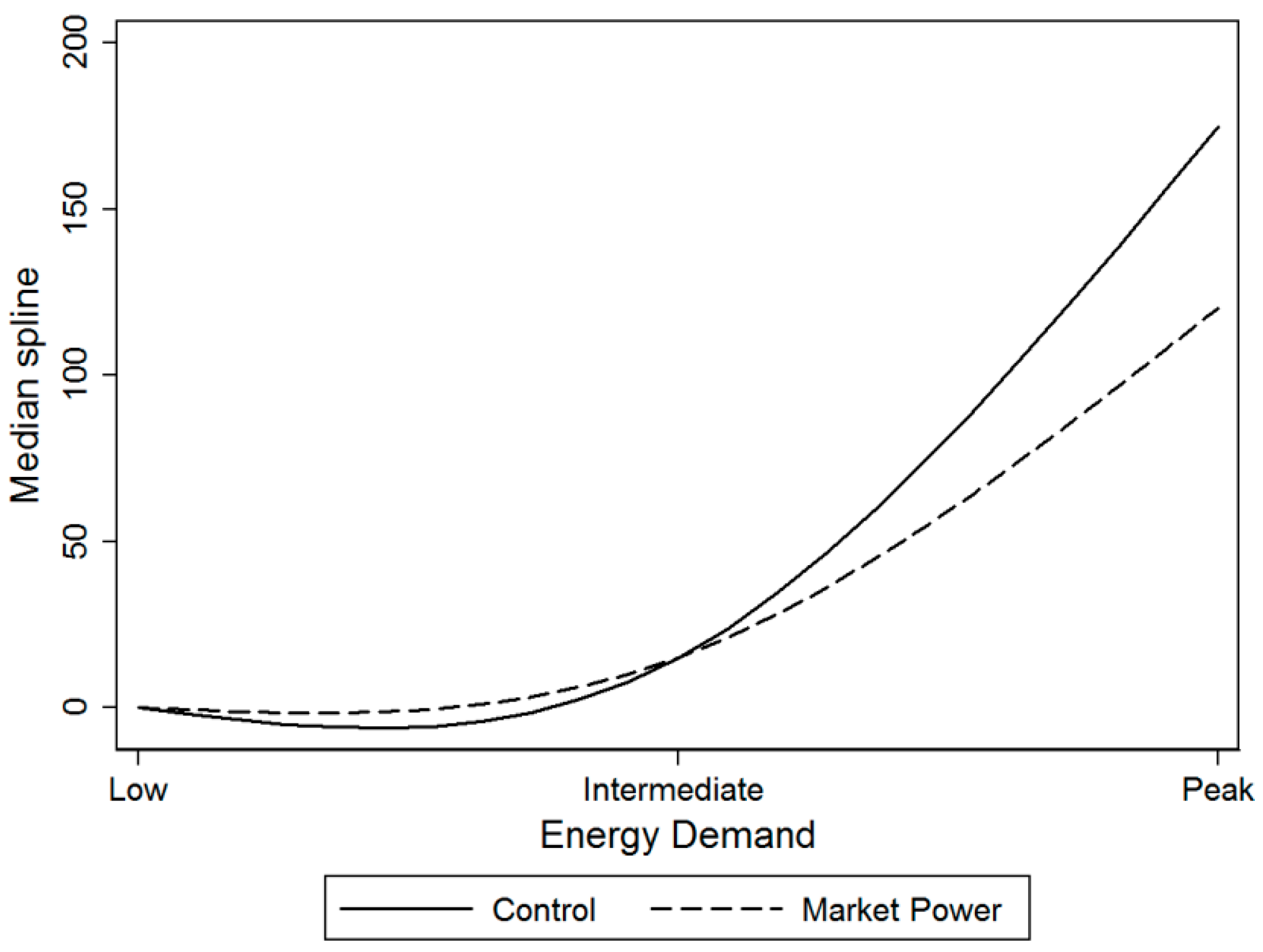
To further analyze Hypothesis 2, a median spline function of revenue (in dollars) is provided in Figure 5. The x-axis of the function provides the three energy demand levels, and the y-axis provides the median spline of government revenue from the simulated carbon auctions. The spline figures provide a graphical assessment of Hypotheses 1 and 2. In particular, it is evident from Figure 5 that market concentration has little effect on government revenue in low and intermediate demand markets. However, the impact becomes much clearer at the peak energy demand level. This is consistent with Hypothesis 2. Figure 6 provides the equivalent function for cases in which firms pursued resale.
As can be seen from Figure 6, Hypothesis 2 is supported at the peak energy demand category as in Figure 5, however a sign change (reversal effect) becomes evident in the low demand markets. Although this positive revenue impact of market power in the low energy market is more than reversed by the negative impact in the peak energy market, the difference illustrates an important feature of resale by dominant firms. That is, when dominant firms purchase allowances for purposes of resale in low demand energy markets, they are not attempting to reduce demand and acquire the emissions permits at a low price, but rather are attempting to corner the market by buying permits required by other firms in the attempt to liquidate them at a profit in subsequent auctions. As such, the effect of market power in low demand energy markets can be to inflate the carbon price where it would otherwise converge toward zero. The distinction between Figure 5 and Figure 6 also provide some illustrative support for Hypothesis 3 regarding resale. While the spline figures do not explicitly highlight temporal differences, the distinction is due to resale, which is an inherent inter-temporal decision among firms.
However, a more formalized test of Hypothesis 3 is provided in Table 4. Table 4 provides Wilcoxon non-parametric hypothesis tests of the null hypothesis corresponding to Hypothesis 3. That is, that the difference in revenue received by the government in the first round auction and revenue received in the second round will be equal regardless of whether resale is pursued by firms. We can safely reject this null hypothesis when treatment conditions are not taken into consideration (p < 0.01). When treatments are not considered, the mean difference in revenue between round 1 and round 2 when resale is pursued is $15.91, and it is $7.77 when resale is not pursued. When treatments are considered, we can safely reject the null at (p < 0.05) in the market power treatment, however we cannot reject the null in the control group. In the control group the mean revenue difference is $6.80 when resale is not pursued and $12.61 when resale is pursued. Although in the expected direction, this test is influenced by the rather small sample size that is an artifact of the experimental design. There was no explicit treatment in which subjects were restricted from resale. Inevitably, in a market consisting of 10 subjects, at least one subject attempted to profit from resale in any given bidding round. In the market power treatment, the mean revenue difference is $8.57 when resale is not pursued and $20.05 when resale is pursued. These provide strong support for Hypothesis 3, particularly in markets defined by market power.
The policy implications of this finding are not immediately apparent from the standpoint of revenue; however they are highly relevant from the standpoint of efficiency and policy implementation. A regulator or state government would not be concerned with differences in revenue between quarterly auctions. However, differences from auction to auction are often compared and measured as metrics of program performance. Skeptics and program evaluators aiming to criticize the overall effectiveness of a trading regime may cite auction-to-auction volatility. However, they may actually be identifying resale effects rather than inherent and underlying volatility due to structural flaws in emissions market design.
5.2. Regression Analysis
To extend the analysis further, regression analysis results are provided in Table 5. The analysis begins with a reduced form model (Model 1) that predicts government revenue from the sale of carbon allowances in the laboratory experiment. An interactive model is then presented in Model 2 that provides a decomposition of the treatment conditions on energy demand levels. Furthermore, the interactive model is extended to include the assessment of resale in Model 3. And finally, Model 4 provides a decomposition of resale by energy demand level. All models utilize Ordinary Least Squares (OLS) regression with heteroskedasticity-corrected robust standard errors [53].
The reduced form model (Model 1) provides a tractable assessment of the treatment effect and energy demand influences on carbon auction revenue. The model however, provides only basic support for Hypotheses 1 and 2 without the decomposition offered in Models 2–4. Model 1 includes a binary indicator variable that indicates the treatment condition for market power, and binary indicator variables for each level of energy demand. Low energy demand is excluded as the reference case.
The treatment dummy for the market power treatment is negative and not statistically significant. Whereas the negative coefficient is in a direction consistent with Hypothesis 1, namely that government revenue is lower under market power, that estimate is not supported at a robust level of statistical significance without further decomposition. The energy demand level variables indicate the change at the mean from government revenue at the low energy demand level. That is, government revenue is $11 experimental higher than government revenue under low energy demand when energy demand is intermediate. Similarly, government revenue is just over $100 experimental higher than government revenue under low energy demand when energy demand is at peak demand. As appropriate, energy demand is significantly and positively associated with government carbon auction revenue, as this represents an inherent demand-side characteristic (see Section 3.3). The reduced form model provides relatively strong summary and fitness measures, as indicated by the R-squared and F-statistic.
The interactive model (Model 2) provides the most support for Hypothesis 1 and Hypothesis 2. The five independent variables of Model 2 include the interaction of each of the three energy demand levels by the associated treatment dummy, with the low energy demand level control group excluded as the reference category. Model 2 also exhibits strong summary and fitness measures. The control group auctions at the intermediate and peak levels of energy demand are larger in magnitude and statistically significant. Compared with the low energy demand level, government revenue was nearly $16 and $125 larger in the intermediate and peak energy demand levels, respectively. This is driven by the demand-side features associated with the positive relationship between energy demand and carbon emissions.
Government revenue in the peak energy demand market under market power is also highly statistically significant, but the coefficient is approximately 33 percent smaller () than the equivalent coefficient for the control group. This provides support for both Hypotheses 1 and 2. Government revenue in the market power treatment at the low and intermediate energy demand levels, however, is slightly above the control group. This is supported by both the descriptive statistics as well as the hypothesis tests in Section 5.1. Taken together, Models 1 and 2 provide support for both hypotheses. Namely, whereas government revenue is less under market power, it is 33 percent less when the demand for energy is high.
These results are driven heavily by the degree of residual demand that the oligopolist maintains in the high energy demand markets. When the energy demand is peak and there is scarcity in the emissions permit market, oligopolists control the largest share of residual demand. Thus, their bids are most likely to be the marginal bid that sets the uniform auction clearing price.
The interactive model is expanded further with Model 3 by the inclusion of resale of emissions allowances. Unlike the binary indicator variables in Models 1 and 2, resale is a levels variable and indicates the quantity of emissions allowances that firms offered for resale into the second round emissions auction. Whereas the coefficient estimate is negative and suggests that government revenue is less when resale is pursued by firms, it fails the statistical significance test.
Model 4 provides an improvement over Model 3 by interacting the energy demand indicators with the levels variable for emissions allowances offered for resale. Again, the low energy demand category is excluded as the reference category. Whereas the coefficient for resale at the intermediate energy demand level is flat and not statistically significant, it is negative and significant at the peak energy demand level. This suggests that for each additional emissions allowance posted for resale by firms in peak energy demand markets, government revenue declines by almost $12 in the experiment. This is consistent with the supply-side features discussed previously.
6. Conclusions
This paper has provided the results of a set of controlled laboratory experiments on the effect of market power in an inter-temporal carbon market. The experiment consisted of a standard 2 treatment design, in which the treatment group provided a moderate market power scenario case and in which the control group provided a more competitive distribution of market share. The treatment group is more closely consistent with state-level and regional energy markets in the U.S. in terms of market concentration. The experiments included many real-world institutional features, including stochastic permit demand from an endogenous energy market with heterogeneous supply portfolios, inter-temporal (two round) carbon auctions within compliance periods, banking of emissions allowances and allowance resale into future auctions.
Three formalized hypotheses regarding the impact of market power on government revenue from the sale of emissions allowances in carbon auctions were provided. These hypotheses were formally tested and confirmed in part, with some important caveats. Namely, carbon auctions defined by market power will tend to yield less government revenue than competitive carbon auctions. Also, the effect of market power on government revenue is significantly larger when the demand for energy is high. It is in these scenarios that dominant firms command an ever larger portion of the residual allowance demand and in which their ability to exercise strategic bidding to influence the price in the carbon auction is greatest. A regression analysis was provided and suggests that governments can expect 33 percent less carbon allowance revenue when the markets are defined by concentration and market power, when the demand for energy is high.
The intuition behind these results is the interdependency between the energy market and the emissions market. When the product market—in this case electricity—is defined by a moderate degree of market concentration (HHI = 2000), peak energy demand markets in which there is scarcity in the emissions permit market provide oligopolists with the largest possible share of residual permit demand. Their ability to exercise price influence over the emissions auction is greatest during peak energy demand because it is during this time of scarcity in the permit market that their bids have the highest expectation of being the marginal bid that sets the uniform auction price.
This paper also considered these impacts for allowance resale. A common feature of emissions auctions in practice today is to allow firms to sell emissions allowances into the auction. This is a policy design feature included to increase liquidity. This paper has provided formalized tests that suggest that allowance resale increases government revenue in early periods and decreases it in later periods, even under a declining emissions cap. This is consistent with firms purchasing allowances for the purpose of resale arbitrage. This has the effect of raising demand for allowances in early auctions and inflating the supply of allowances in later auctions into which the allowances are resold. Whereas these results are instructive in explaining the declining price effects in regional carbon markets like RGGI, it is expected that over a significantly longer time horizon, such as a three year compliance period, and with banking across compliance periods, these effects would ebb away.
Whereas the European Union maintains a robust international carbon market, no such national market exists in the U.S. The implications of this paper are particularly important for the U.S., in which current carbon markets in California and the RGGI (nine East Coast states) are defined by greater concentration among firms and in which only the energy sector participates in the carbon market on a non-voluntary basis. However, the implications of this paper are also important to the European Union ETS markets, which have a directive to begin using auctions as a method for allocating emissions permits beginning in the next phase (similar to a compliance period in the U.S.) of the program.
Finally, the results are also highly relevant for purposes of federal planning for national carbon regulatory design. Stemming from the 2007 U.S. Supreme Court’s endangerment finding in Massachusetts v. EPA (549 U.S. 497), the Environmental Protection Agency (EPA) has put forth regulations for greenhouse gas emissions from existing power facilities under the Clean Air Act (Section 111d) under President Obama’s Clean Power Plan. Under the Plan, states are the compliance entities and have a variety of approaches at their disposal for compliance with the mandate. The Plan recommends market-based approaches modeled after RGGI and California’s program as the first recommendation. As such, the sale of carbon permits through a regional or state-level carbon market represents a compliance approach that also yields revenue to state governments. The implications of this paper would suggest therefore, that if states such as New Mexico operate their own auction-based carbon market modeled after California or RGGI, they can expect substantially less revenue than that which would be predicted under competitive market assumptions.
Acknowledgments
The author thanks the John Randolph and Dora Haynes Foundation for its generous financial support.
Conflicts of Interest
The authors declare no conflict of interest.
References and Notes
- Dales, J. Pollution, Property and Prices; University Press: Toronto, ON, Canada, 1968. [Google Scholar]
- Montgomery, W.D. Markets for licenses and pollution control. J. Econ. Theory. 1972, 5, 395–418. [Google Scholar] [CrossRef]
- Tietenberg, T.H. Emissions Trading: Principles and Practice, 2nd ed.; Resources for the Future Press: Washington, DC, USA, 2006. [Google Scholar]
- Tietenberg, T.; Lewis, L. Environmental and Natural Resource Economics, 9th ed.; Routledge: New York, NY, USA, 2012. [Google Scholar]
- Dormady, N.; Englander, A. Carbon allowances and the demand for offsets: A comprehensive assessment of imperfect substitutes. J. Public Policy 2016, 36, 139–167. [Google Scholar] [CrossRef]
- Borenstein, S.; Bushnell, J.; Knittel, C.; Wolfram, C. Inefficiencies and market power in financial arbitrage: A study of California’s electricity markets. J. Ind. Econ. 2008, 56, 347–378. [Google Scholar] [CrossRef]
- Brennan, T.J. Preventing Monopoly or Discouraging Competition? The Perils of Price-Cost Tests for Market Power in Electricity. In Electric Choices: Deregulation and the Future of Electric Power; Kleit, A.N., Ed.; Rowman & Littlefield: Lanham, MD, USA, 2006. [Google Scholar]
- Hortacsu, A.; Puller, S. Understanding strategic bidding in multi-unit auctions: A case study of the Texas electricity spot market. RAND J. Econ. 2008, 39, 86–114. [Google Scholar] [CrossRef]
- Hunt, S. Making Competition Work in Electricity; John Wiley & Sons: New York, NY, USA, 2002. [Google Scholar]
- Joskow, P.L. Restructuring, competition and regulatory reform in the U.S. electricity sector. In Designing Competitive Electricity Markets; Chao, H., Huntington, H.G., Eds.; Kluwer Press: Boston, MA, USA, 1998; pp. 11–31. [Google Scholar]
- Joskow, P.L.; Kahn, E. A quantitative analysis of pricing behavior in California’s wholesale electricity market during summer 2000: The final word. Energy J. 2002, 23, 1–35. [Google Scholar] [CrossRef]
- Perekhodtsev, D.; Baselice, R. Empirical assessment of strategic behavior in the Italian power exchange. Eur. Trans. Electr. Power 2010, 21, 1842–1855. [Google Scholar] [CrossRef]
- Saravia, C. Speculative Trading and Market Performance: The Effect of Arbitrageurs on Efficiency and Market Power in the New York Electricity Market; Working Paper 121; University of California (Berkeley), Center for the Study of Energy Markets: Berkeley, CA, USA, 2003. [Google Scholar]
- Alvarez, F.; Andre, F.J. Auctioning versus grandfathering in cap-and-trade systems with market power and incomplete information. Environ. Resour. Econ. 2015, 62, 1–34. [Google Scholar] [CrossRef]
- Burtraw, D.; Goeree, J.; Holt, C.A.; Myers, E.; Palmer, K.; Shobe, W. Collusion in Auctions for Emissions Permits: An Experimental Analysis; Working Paper DP 08-36; Resources for the Future: Washington, DC, USA, 2008. [Google Scholar]
- Chavez, C.A.; Stranlund, J.K. Enforcing transferable permit systems in the presence of market power. Environ. Resour. Econ. 2003, 25, 65–78. [Google Scholar] [CrossRef]
- Dormady, N. Market power in cap-and-trade auctions: A Monte Carlo approach. Energy Policy 2013, 62, 788–797. [Google Scholar] [CrossRef]
- Godby, R. Market power and emissions trading: Theory and laboratory results. Pac. Econ. Rev. 2000, 5, 349–363. [Google Scholar] [CrossRef]
- Hahn, R.W. Market power and transferable property rights. Q. J. Econ. 1984, 99, 763–765. [Google Scholar] [CrossRef]
- Lange, A. On the endogeneity of market power in emissions markets. Environ. Resour. Econ. 2012, 52, 573–583. [Google Scholar] [CrossRef]
- Liski, M.; Montero, J.P. On pollution permit banking and market power. J. Regul. Econ. 2006, 29, 283–302. [Google Scholar] [CrossRef]
- Malik, A.S. Further results on permit markets with market power and cheating. J. Environ. Econ. Manag. 2002, 44, 371–390. [Google Scholar] [CrossRef]
- Misiolek, W.S.; Elder, H.W. Exclusionary manipulation of markets for pollution rights. J. Environ. Econ. Manag. 1989, 16, 156–166. [Google Scholar] [CrossRef]
- Van Egteren, H.; Weber, M. Marketable permits, market power, and cheating. J. Environ. Econ. Manag. 1996, 30, 161–173. [Google Scholar] [CrossRef]
- California’s program is slated to add petroleum refiners in 2016. This addition is the subject of intense political debate and is challenged in the courts presently.
- Borenstein, S.; Bushnell, J.; Wolak, F.A. Measuring market inefficiencies in California’s restructured wholesale electricity market. Am. Econ. Rev. 2002, 92, 1376–1405. [Google Scholar] [CrossRef]
- Kolstad, J.; Wolak, F. Using Environmental Emissions Permit Prices to Raise Electricity Prices: Evidence from the California Electricity Market; Working Paper WP 113; University of California, Center for the Study of Energy Markets: Berkeley, CA, USA, 2003. [Google Scholar]
- Limpaitoon, T.; Chen, Y.H.; Oren, S. The impact of imperfect competition in emission permits trading on oligopolistic electricity markets. Energy J. 2014, 35, 145–166. [Google Scholar] [CrossRef]
- Reichenbach, J.; Requate, T. Potential Anti-Competitive Effects of Emission Permit Markets: A Survey on Theoretical Findings and Evidence. Rev. Econ. 2013, 64, 271–292. [Google Scholar] [CrossRef]
- Sartzetakis, E.S. Tradeable emission permits regulations in the presence of imperfectly competitive product markets: Welfare implications. Environ. Resour. Econ. 1997, 9, 65–81. [Google Scholar] [CrossRef]
- Dormady, N. Carbon auctions, energy markets and market power: An experimental analysis. Energy Econ. 2014, 44, 468–482. [Google Scholar] [CrossRef]
- Investigating the Impact of Nuclear Power Plant License Renewal. Power Point Presentation to the Regional Greenhouse Gas Initiative (RGGI) Inc., September 2005. Available online: http://www.rggi.org/docs/epri_charts_9_9_05.ppt (accessed on 20 July 2016).
- Engelbrecht-Wiggans, R.; List, J.A.; Lucking-Reiley, D. Demand reduction in multi-unit auctions with varying numbers of bidders: Theory and evidence from a field experiment. Int. Econ. Rev. 2006, 47, 203–231. [Google Scholar] [CrossRef]
- Hintermann, B. Market power, permit allocation and efficiency in emission permit markets. Environ. Resour. Econ. 2011, 49, 327–349. [Google Scholar] [CrossRef]
- Von der Fehr, N.M. Tradeable emission rights and strategic interaction. Environ. Resour. Econ. 1993, 3, 129–151. [Google Scholar] [CrossRef]
- This was also the auction format proscribed in the U.S. proposals in the Senate (Kerry-Boxer) and House of Representatives (Waxman-Markey) in 2009; S. 1733 (http://www.c2es.org/federal/congress/111/clean-energy-jobs-american-power-act) and H.R. 2454 (https://www.congress.gov/bill/111th-congress/house-bill/2454), respectively.
- Uniform price auctions vary widely in their decision rule regarding which bid sets the market price. Some uniform price auctions set the market price as the lowest winning bid, while others set the uniform price as the highest losing bid. The latter is referred to as a second price mechanism. The interested reader is encouraged to see Krishna (2009) [38].
- Krishna, V. Auction Theory, 2nd ed.; Elsevier Press: Oxford, UK, 2009. [Google Scholar]
- Stevens, B.; Rose, A. A dynamic analysis of the marketable permits approach to global warming policy: A comparison of spatial and temporal flexibility. J. Environ. Econ. Manag. 2002, 44, 45–69. [Google Scholar] [CrossRef]
- The decision rule utilized for ties in both the energy and emissions auctions was randomization. The decision rule utilized for ties in the resale market (e.g., four permits were posed for resale by two subjects but only three of them sold) was weighted averaging in which weights were given by the proportion of total resale permits posted into the auction by an individual reseller.
- Ellerman, A.D.; Schmalensee, R.; Bailey, E.M.; Joskow, P.L.; Montero, J.P. Markets for Clean Air: The U.S. Acid Rain Program; Cambridge University Press: Cambridge, UK, 2000. [Google Scholar]
- The Herfindahl–Hirschman Index (HHI) is the U.S. Department of Justice’s measure of market concentration. It ranges from 10,000 in the case of a perfect monopoly, and approaches zero in an atomistic market. According to recent guidelines, any HHI above 1800 is a moderately concentrated market. See Dormady (2013) for an assessment of the HHI in recent carbon auctions.
- TechSmith. Jing Pro, Computer Software; TechSmith: Okemo, MI, USA, 2011.
- Fischbacher, U. Z-TREE: Zurich Tookbox for Ready-made Economic Experiments. Exp. Econ. 2007, 10, 171–178. [Google Scholar] [CrossRef]
- Gale, I.L.; Hausch, D.B. Bottom-fishing and declining prices in sequential auctions. Games Econ. Behav. 1994, 7, 318–331. [Google Scholar] [CrossRef]
- McAfee, R.P.; Vincent, D. The declining price anomaly. J. Econ. Theory 1993, 60, 191–212. [Google Scholar] [CrossRef]
- Milgrom, P.; Webber, R.J. A Theory of Auctions and Competitive Bidding, II. In The Economic Theory of Auctions; Klemperer, P., Ed.; Edward Elgar Publishing, Ltd.: Cheltenham, UK, 2000; Volume 2, pp. 179–194. [Google Scholar]
- Weber, R.J. Multiple Object Auctions. In Auctions, Bidding, and Contracting: Uses and Theory; Engelbrecht-Wiggans, R., Shubik, M., Stark, R.M., Eds.; New York University Press: New York, NY, USA, 1983; pp. 165–191. [Google Scholar]
- One significant mitigating factor, not simulated here, is the effect of trading in the secondary market. This can occur through a brokerage or on a bilateral basis, depending upon the rules of the regional market. However, the same general results occur in the instance of a secondary trading market. That is, government revenue is inflated when allowances are purchased for purposes of resale, and suppressed when those permits are liquidated on either the secondary market or through the auction.
- Electric Reliability Council of Texas. 2010 State of the Market Report for the ERCOT Wholesale Electricity Markets. 2010. Available online: http://www.potomaceconomics.com/uploads/ercot_reports/2010_ERCOT_SOM_REPORT.pdf (accessed on 20 July 2016).
- PJM. State of the Market Report for PJM, Volume II: Detailed Analysis. 2012. Available online: http://www.monitoringanalytics.com/reports/PJM_State_of_the_Market/2011.shtml (accessed on 20 July 2016).
- It should be noted that these lower bound market power scenarios assume full and perfect collusion among the two oligopolists.
- Davidson, R.; MacKinnon, J.G. Estimation and Inference in Econometrics; Oxford University Press: New York, NY, USA, 1993. [Google Scholar]
Figure 1.
Government over-allocation of emissions allowances in the New England carbon market (Note: Values in Figure 1 are the state by state difference between reported 2008 emissions from the Regional Greenhouse Gas Initiative (RGGI) carbon inventory and state final allowance allocations (issued allowances); Over-Allocation = Allowances Issued—2008 Emissions Inventory.). CT: Connecticut; DE: Delaware; MA: Massachusetts; MD: Maryland; ME: Maine; NH: New Hampshire; NJ: New Jersey; NY: New York; RI: Rhode Island; VT: Vermont.

Figure 2.
Government over-allocation of emissions allowances in the New England carbon market (Note: Values in Figure 2 are the state by state difference between reported 2000–2008 emissions from RGGI carbon inventory and state final allowance allocations (issued allowances); Over-Allocation = Allowances Issued—Annual Average 2000–2008 Emissions Inventory.).

Figure 3.
Market concentration and auction price in New England carbon auctions.

Figure 4.
Box plot of government revenue by treatment.

Figure 5.
Median spline of treatment effect (no allowance resale).

Figure 6.
Median spline of treatment effect (with resale).


| Treatment | Energy Demand | Carbon Auction Revennue | ||||
|---|---|---|---|---|---|---|
| Mean | S.D. | Min. | Max. | N | ||
| Control | Low | $9.69 | 15.21 | 0.00 | 59.80 | 19 |
| Intermediate | $25.40 | 26.21 | 0.00 | 117.15 | 28 | |
| Peak | $133.70 | 34.57 | 69.00 | 186.25 | 30 | |
| Treatment (Market Power) | Low | $19.46 | 20.45 | 0.00 | 65.00 | 25 |
| Intermediate | $29.96 | 31.77 | 0.00 | 104.20 | 22 | |
| Peak | $93.71 | 37.55 | 20.00 | 154.85 | 30 | |
Note: Figures in experimental dollar terms.
| Treatment | Resale | Energy Demand | Carbon Auction Revennue | ||||
|---|---|---|---|---|---|---|---|
| Mean | S.D. | Min. | Max. | N | |||
| Control | No Resale | Low | $0.00 | 0.00 | 0.00 | 0.00 | 4 |
| Intermediate | $20.45 | 21.06 | 1.80 | 50.00 | 4 | ||
| Peak | $157.80 | 32.59 | 100.00 | 174.85 | 5 | ||
| Treatment (Market Power) | Low | $3.33 | 8.14 | 0.00 | 19.95 | 6 | |
| Intermediate | $13.09 | 12.46 | 0.00 | 26.00 | 5 | ||
| Peak | $116.23 | 40.66 | 63.00 | 154.85 | 5 | ||
| Control | Resale | Low | $12.28 | 16.26 | 0.00 | 59.80 | 15 |
| Intermediate | $26.23 | 27.27 | 0.00 | 117.15 | 24 | ||
| Peak | $128.88 | 33.49 | 69.00 | 186.25 | 25 | ||
| Treatment (Market Power) | Low | $24.56 | 20.61 | 0.00 | 65.00 | 19 | |
| Intermediate | $34.93 | 34.22 | 2.00 | 104.20 | 17 | ||
| Peak | $86.20 | 34.63 | 20.00 | 138.60 | 15 | ||
| Null Hypothesis | Demand | Z-Value | p-Value |
|---|---|---|---|
| Revenue (Control) = Revenue (Treatment) | Peak | 3.37 *** | 0.001 |
| Intermediate | −0.37 | 0.709 | |
| Low | −0.14 | 0.255 | |
| Revenue (Control) = Revenue (Treatment) (Round 1) | Peak | 2.64 ** | 0.007 |
| Intermediate | −0.65 | 0.517 | |
| Low | −1.17 | 0.243 | |
| Revenue (Control) = Revenue (Treatment) (Round 2) | Peak | 2.97 ** | 0.003 |
| Intermediate | 0.66 | 0.509 | |
| Peak | −1.09 | 0.273 |
Notes: * p < 0.05; ** p < 0.01; *** p < 0.001.
| Null Hypothesis | Treatment | Z-Value | p-Value |
|---|---|---|---|
| Revenue R1 – Revenue R2 (No Resale) = Revenue R1 – Revenue R2 (Resale) | All | −2.60 ** | 0.009 |
| Treatment | −2.18 * | 0.029 | |
| Control | −1.19 | 0.231 |
Notes: * p < 0.05; ** p < 0.01; *** p < 0.001.
| Explanatory Variables | Model 1 | Model 2 | Model 3 | Model 4 |
|---|---|---|---|---|
| Market Power Treatment | −9.06 | - | - | - |
| [−5.36] | - | - | - | |
| Intermediate Energy Demand | 11.0 * | - | - | - |
| [5.34] | - | - | - | |
| Peak Energy Demand | 100.93 *** | - | - | - |
| [6.49] | - | - | - | |
| Control * Intermediate Energy Demand | - | 15.71 * | 16.02 * | 15.32 * |
| - | [6.19] | [6.56] | [7.25] | |
| Control * Peak Energy Demand | - | 124.01 *** | 122.72 *** | 148.22 *** |
| - | [7.35] | [7.47] | [8.17] | |
| Market Power * Low Energy Demand | - | 9.77 | 9.08 | 9.77 |
| - | [5.50] | [5.89] | [5.50] | |
| Market Power * Intermediate Energy Demand | - | 20.27 ** | 19.16 * | 20.05 * |
| - | [7.81] | [7.98] | [8.04] | |
| Market Power * Peak Energy Demand | - | 84.01 *** | 82.79 *** | 109.03 *** |
| - | [9.33] | [9.37] | [9.79] | |
| Resale | - | - | −0.86 | - |
| - | - | [−0.67] | - | |
| Resale * Intermediate Energy Demand | - | - | - | 0.10 |
| - | - | - | 0.65 | |
| Resale * Peak Energy Demand | - | - | - | −11.92 *** |
| - | - | - | [−2.53] | |
| Constant | 20.39 *** | 9.69 ** | 12.73 ** | 9.69 ** |
| [4.25] | [3.59] | [4.37] | [3.59] | |
| N | 144 | 144 | 144 | 144 |
| F | 90.13 *** | 70.10 *** | 58.78 *** | 72.47 *** |
| R2 | 0.69 | 0.74 | 0.74 | 0.79 |
Note: OLS regression models with robust heteroskedasticity corrected standard errors in brackets, * p < 0.05; ** p < 0.01; *** p < 0.001.
© 2016 by the author; licensee MDPI, Basel, Switzerland. This article is an open access article distributed under the terms and conditions of the Creative Commons Attribution (CC-BY) license (http://creativecommons.org/licenses/by/4.0/).
Share and Cite
MDPI and ACS Style
Dormady, N. Carbon Auction Revenue and Market Power: An Experimental Analysis. Energies 2016, 9, 897. https://0-doi-org.brum.beds.ac.uk/10.3390/en9110897
AMA Style
Dormady N. Carbon Auction Revenue and Market Power: An Experimental Analysis. Energies. 2016; 9(11):897. https://0-doi-org.brum.beds.ac.uk/10.3390/en9110897
Chicago/Turabian StyleDormady, Noah. 2016. "Carbon Auction Revenue and Market Power: An Experimental Analysis" Energies 9, no. 11: 897. https://0-doi-org.brum.beds.ac.uk/10.3390/en9110897
Note that from the first issue of 2016, this journal uses article numbers instead of page numbers. See further details here.