Hybrid Machine Learning Approaches for Landslide Susceptibility Modeling


 , , ,
, , ,  , ,
, ,  and
and
Abstract
:1. Introduction
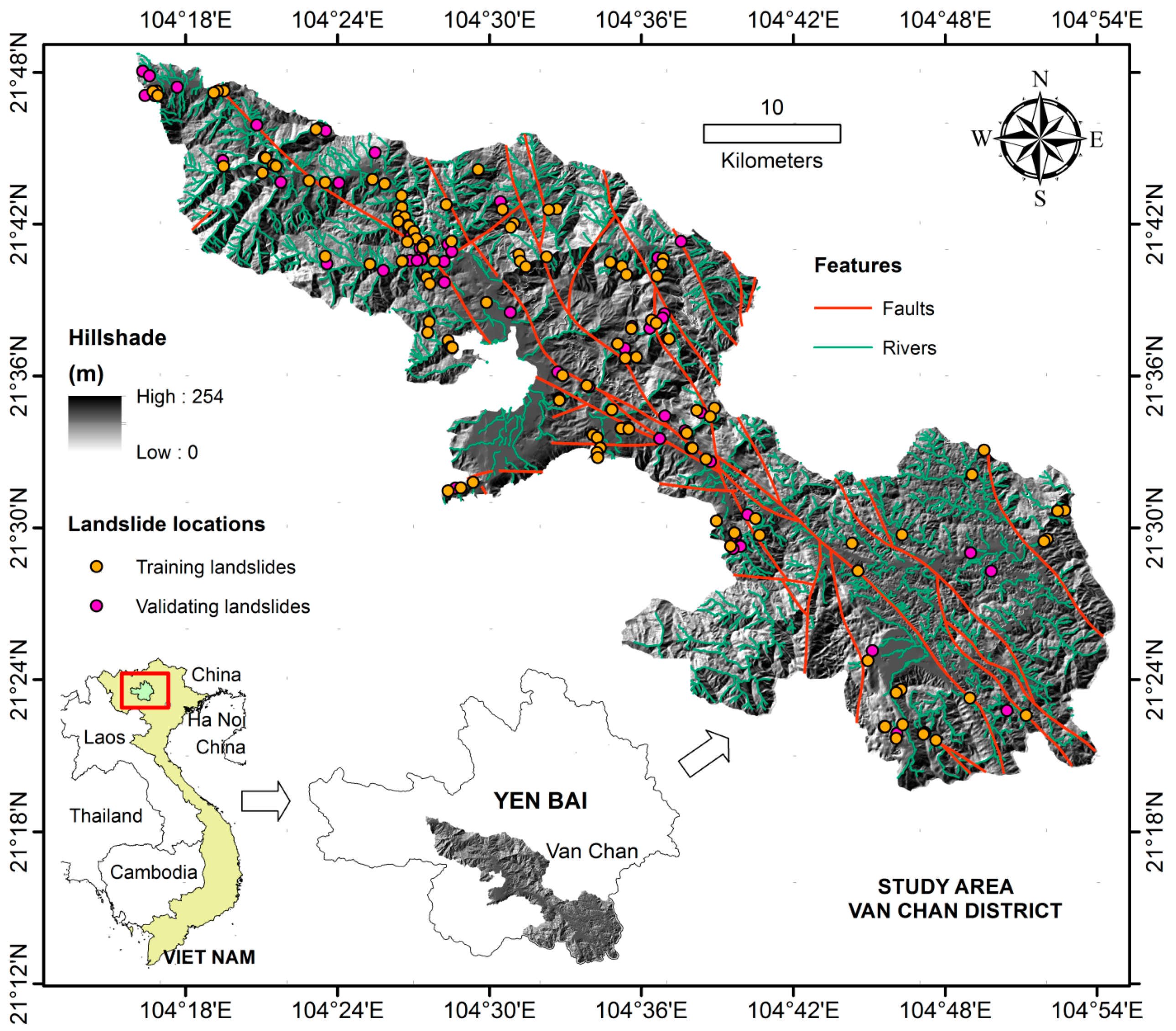
2. Study Area
3. Materials and Methods
3.1. Data Used
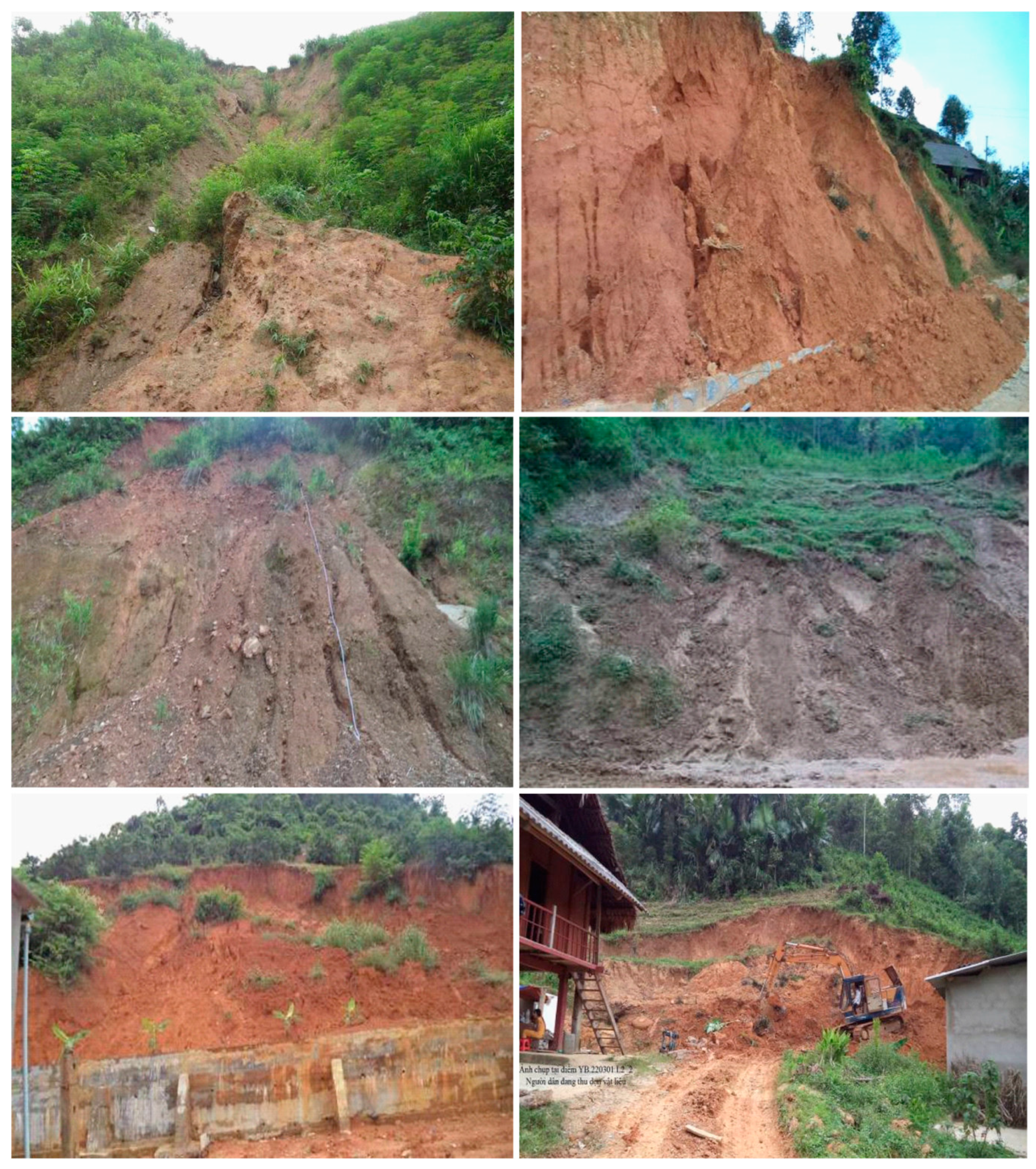
3.1.1. Landslide Inventory
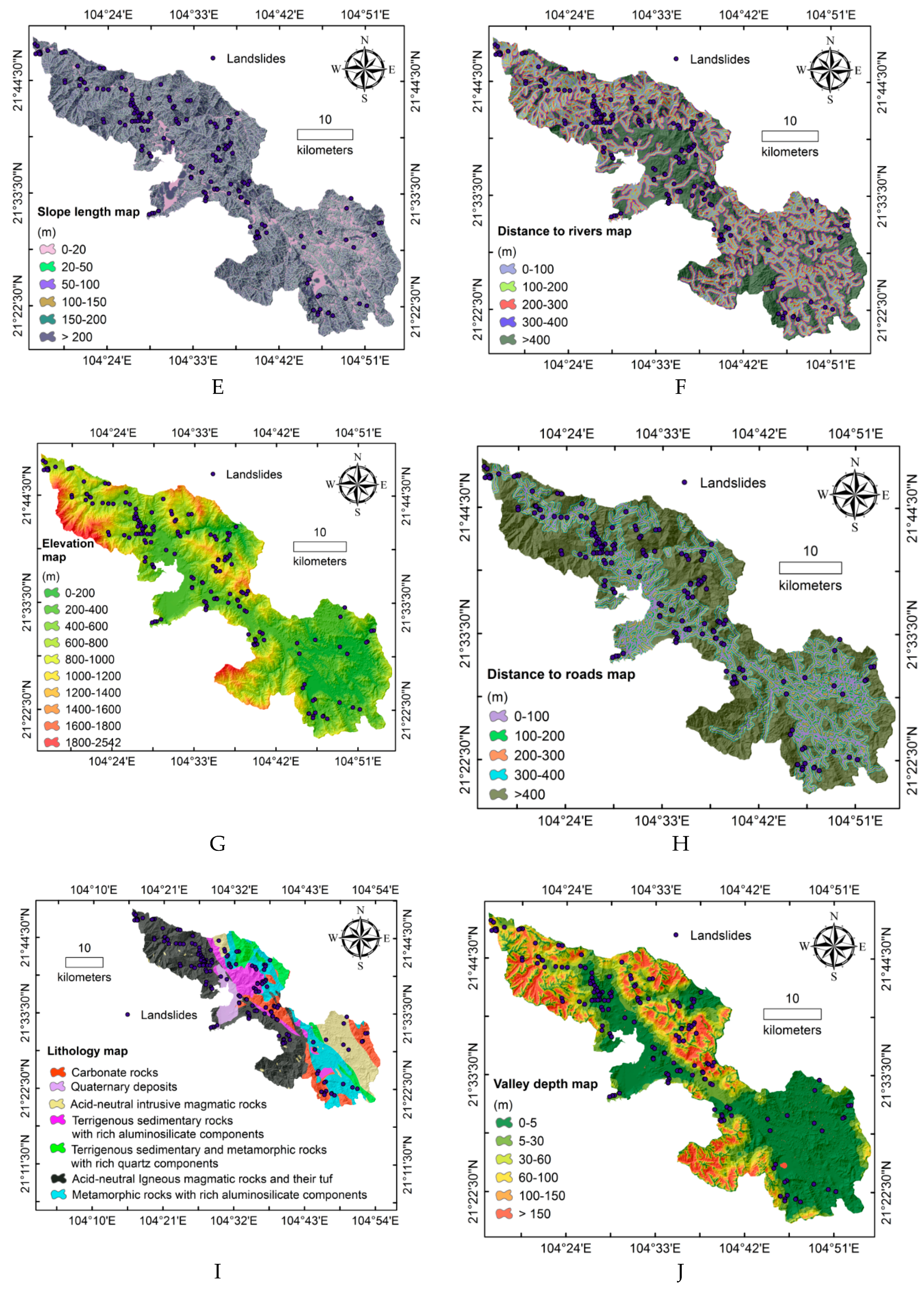
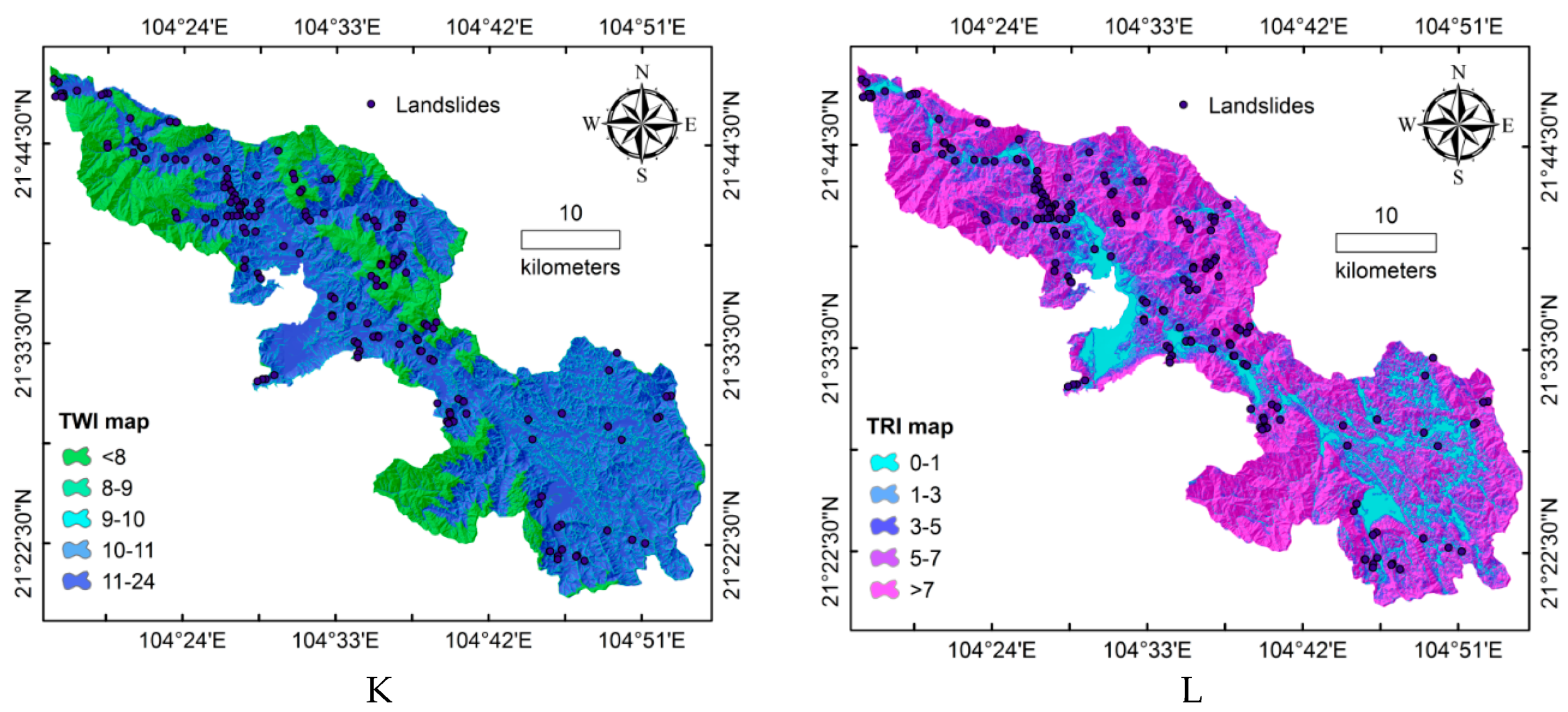
3.1.2. Landslide Influencing Parameters
3.2. Methods Used
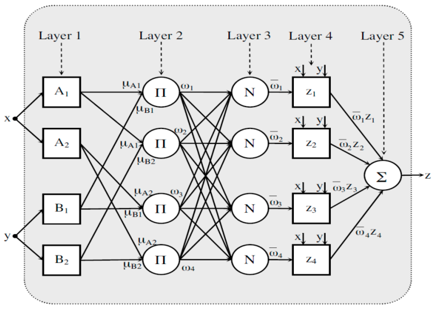
3.2.1. Adaptive Neuro Fuzzy Inference System (ANFIS)
3.2.2. Multilayer Perceptron Neural Networks
3.2.3. Particle Swarm Optimization (Pso)
3.2.4. Rotation Forest
3.2.5. Best First Decision Trees
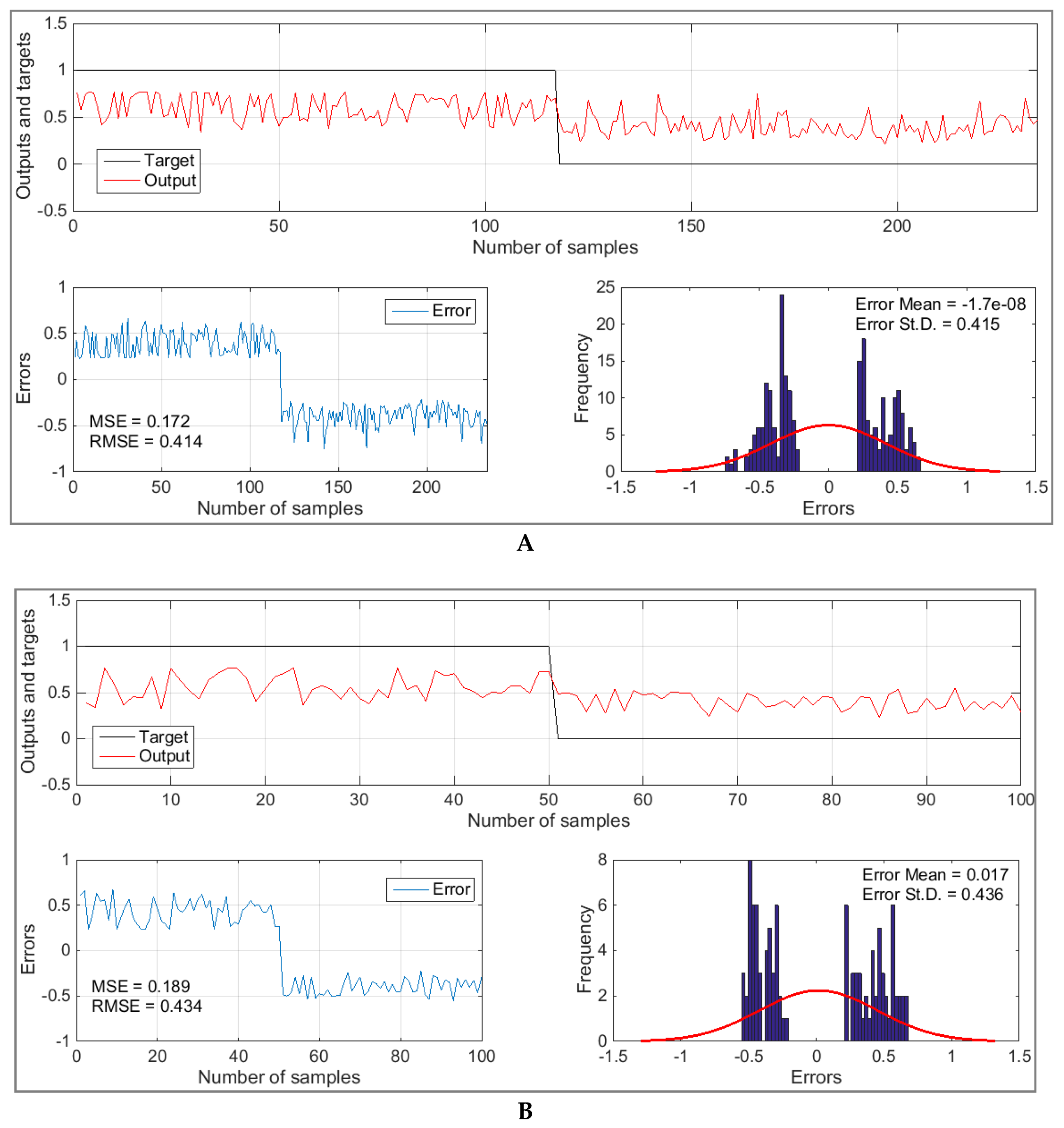
3.2.6. Validation Assessment
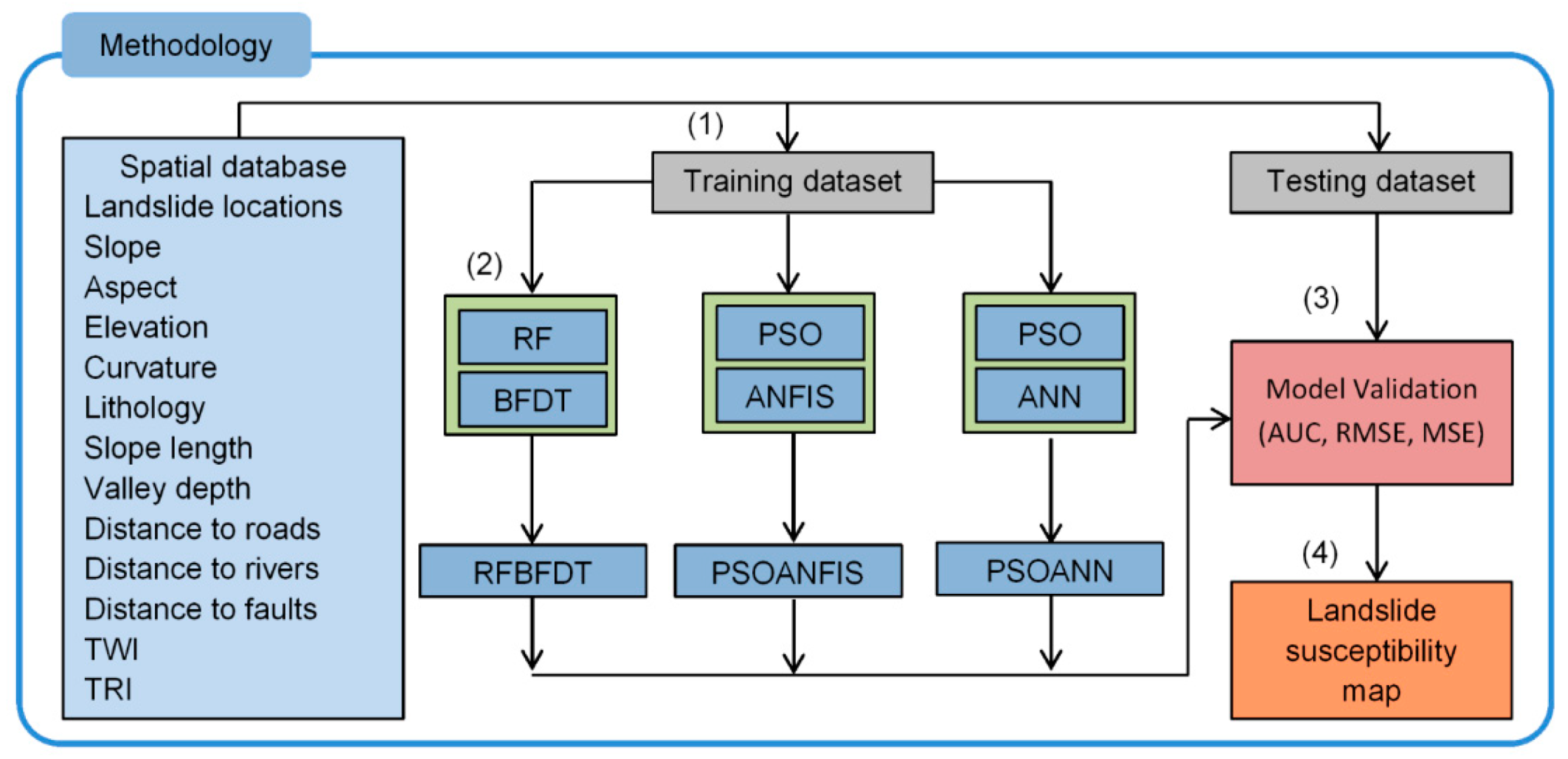
4. Methodology Adopted for Developing Landslide Susceptibility Maps
5. Results and Discussion
6. Conclusions
Author Contributions
Funding
Acknowledgments
Conflicts of Interest
References
- Cruden, D.M. A simple definition of a landslide. Bull. Eng. Geol. Environ. 1991, 43, 27–29. [Google Scholar] [CrossRef]
- Fell, R.; Corominas, J.; Bonnard, C.; Cascini, L.; Leroi, E.; Savage, W.Z. Guidelines for landslide susceptibility, hazard and risk zoning for land use planning. Eng. Geol. 2008, 102, 85–98. [Google Scholar] [CrossRef] [Green Version]
- Ercanoglu, M.; Gokceoglu, C. Use of fuzzy relations to produce landslide susceptibility map of a landslide prone area (West Black Sea Region, Turkey). Eng. Geol. 2004, 75, 229–250. [Google Scholar] [CrossRef]
- Song, Y.; Gong, J.; Gao, S.; Wang, D.; Cui, T.; Li, Y.; Wei, B. Susceptibility assessment of earthquake-induced landslides using Bayesian network: A case study in Beichuan, China. Comput. Geosci. 2012, 42, 189–199. [Google Scholar] [CrossRef]
- Pradhan, B. A comparative study on the predictive ability of the decision tree, support vector machine and neuro-fuzzy models in landslide susceptibility mapping using GIS. Comput. Geosci. 2013, 51, 350–365. [Google Scholar] [CrossRef] [Green Version]
- Bui, D.T.; Pradhan, B.; Lofman, O.; Revhaug, I.; Dick, O.B. Landslide susceptibility mapping at Hoa Binh province (Vietnam) using an adaptive neuro-fuzzy inference system and GIS. Comput. Geosci. 2012, 45, 199–211. [Google Scholar]
- Umar, Z.; Pradhan, B.; Ahmad, A.; Jebur, M.N.; Tehrany, M.S. Earthquake induced landslide susceptibility mapping using an integrated ensemble frequency ratio and logistic regression models in West Sumatera Province, Indonesia. Catena 2014, 118, 124–135. [Google Scholar] [CrossRef]
- Su, C.; Wang, L.; Wang, X.; Huang, Z.; Zhang, X. Mapping of rainfall-induced landslide susceptibility in Wencheng, China, using support vector machine. Nat. Hazards 2015, 76, 1759–1779. [Google Scholar] [CrossRef]
- Chen, W.; Yan, X.; Zhao, Z.; Hong, H.; Bui, D.T.; Pradhan, B. Spatial prediction of landslide susceptibility using data mining-based kernel logistic regression, naive Bayes and RBFNetwork models for the Long County area (China). Bull. Eng. Geol. Environ. 2018, 1–20. [Google Scholar] [CrossRef]
- Youssef, A.M.; Pourghasemi, H.R.; Pourtaghi, Z.S.; Al-Katheeri, M.M. Landslide susceptibility mapping using random forest, boosted regression tree, classification and regression tree, and general linear models and comparison of their performance at Wadi Tayyah Basin, Asir Region, Saudi Arabia. Landslides 2016, 13, 839–856. [Google Scholar] [CrossRef]
- Dou, J.; Yamagishi, H.; Pourghasemi, H.R.; Yunus, A.P.; Song, X.; Xu, Y.; Zhu, Z. An integrated artificial neural network model for the landslide susceptibility assessment of Osado Island, Japan. Nat. Hazards 2015, 78, 1749–1776. [Google Scholar] [CrossRef]
- Chen, W.; Zhang, S.; Li, R.; Shahabi, H. Performance evaluation of the gis-based data mining techniques of best-first decision tree, random forest, and naïve bayes tree for landslide susceptibility modeling. Sci. Total Environ. 2018, 644, 1006–1018. [Google Scholar] [CrossRef]
- Pham, B.T.; Prakash, I. Machine Learning Methods of Kernel Logistic Regression and Classification and Regression Trees for Landslide Susceptibility Assessment at Part of Himalayan Area, India. Indian J. Sci. Technol. 2018, 11. [Google Scholar] [CrossRef]
- Abedini, M.; Ghasemian, B.; Shirzadi, A.; Shahabi, H.; Chapi, K.; Pham, B.T.; Bin Ahmad, B.; Tien Bui, D. A novel hybrid approach of bayesian logistic regression and its ensembles for landslide susceptibility assessment. Geocarto Int. 2018, 1–31. [Google Scholar] [CrossRef]
- Zhang, T.; Han, L.; Chen, W.; Shahabi, H. Hybrid Integration Approach of Entropy with Logistic Regression and Support Vector Machine for Landslide Susceptibility Modeling. Entropy 2018, 20, 884. [Google Scholar] [CrossRef]
- Chen, W.; Shahabi, H.; Zhang, S.; Khosravi, K.; Shirzadi, A.; Chapi, K.; Pham, B.; Zhang, T.; Zhang, L.; Chai, H. Landslide susceptibility modeling based on gis and novel bagging-based kernel logistic regression. Appl. Sci. 2018, 8, 2540. [Google Scholar] [CrossRef]
- Hoang, N.-D.; Tien Bui, D. A novel relevance vector machine classifier with cuckoo search optimization for spatial prediction of landslides. J. Comput. Civ. Eng. 2016, 30, 04016001. [Google Scholar] [CrossRef]
- Chen, W.; Pourghasemi, H.R.; Naghibi, S.A. A comparative study of landslide susceptibility maps produced using support vector machine with different kernel functions and entropy data mining models in China. Bull. Eng. Geol. Environ. 2018, 77, 647–664. [Google Scholar] [CrossRef]
- Pourghasemi, H.R.; Pradhan, B.; Gokceoglu, C. Application of fuzzy logic and analytical hierarchy process (AHP) to landslide susceptibility mapping at Haraz watershed, Iran. Nat. Hazards 2012, 63, 965–996. [Google Scholar] [CrossRef]
- Jebur, M.N.; Pradhan, B.; Tehrany, M.S. Manifestation of LiDAR-derived parameters in the spatial prediction of landslides using novel ensemble evidential belief functions and support vector machine models in GIS. IEEE J. Sel. Top. Appl. Earth Obs. Remote Sens. 2015, 8, 674–690. [Google Scholar] [CrossRef]
- Meinhardt, M.; Fink, M.; Tünschel, H. Landslide susceptibility analysis in central Vietnam based on an incomplete landslide inventory: Comparison of a new method to calculate weighting factors by means of bivariate statistics. Geomorphology 2015, 234, 80–97. [Google Scholar] [CrossRef]
- Gomez, H.; Kavzoglu, T. Assessment of shallow landslide susceptibility using artificial neural networks in Jabonosa River Basin, Venezuela. Eng. Geol. 2005, 78, 11–27. [Google Scholar] [CrossRef]
- Bai, S.; Lü, G.; Wang, J.; Zhou, P.; Ding, L. GIS-based rare events logistic regression for landslide-susceptibility mapping of Lianyungang, China. Environ. Earth Sci. 2011, 62, 139–149. [Google Scholar] [CrossRef]
- Lee, S.; Min, K. Statistical analysis of landslide susceptibility at Yongin, Korea. Environ. Geol. 2001, 40, 1095–1113. [Google Scholar] [CrossRef]
- Galli, M.; Ardizzone, F.; Cardinali, M.; Guzzetti, F.; Reichenbach, P. Comparing landslide inventory maps. Geomorphology 2008, 94, 268–289. [Google Scholar] [CrossRef]
- Yilmaz, I. Comparison of landslide susceptibility mapping methodologies for Koyulhisar, Turkey: Conditional probability, logistic regression, artificial neural networks, and support vector machine. Environ. Earth Sci. 2010, 61, 821–836. [Google Scholar] [CrossRef]
- Ermini, L.; Catani, F.; Casagli, N. Artificial neural networks applied to landslide susceptibility assessment. Geomorphology 2005, 66, 327–343. [Google Scholar] [CrossRef]
- Ayalew, L.; Yamagishi, H. The application of GIS-based logistic regression for landslide susceptibility mapping in the Kakuda-Yahiko Mountains, Central Japan. Geomorphology 2005, 65, 15–31. [Google Scholar] [CrossRef]
- Demir, G.; Aytekin, M.; Akgün, A.; Ikizler, S.B.; Tatar, O. A comparison of landslide susceptibility mapping of the eastern part of the North Anatolian Fault Zone (Turkey) by likelihood-frequency ratio and analytic hierarchy process methods. Nat. Hazards 2013, 65, 1481–1506. [Google Scholar] [CrossRef]
- Nefeslioglu, H.A.; Duman, T.Y.; Durmaz, S. Landslide susceptibility mapping for a part of tectonic Kelkit Valley (Eastern Black Sea region of Turkey). Geomorphology 2008, 94, 401–418. [Google Scholar] [CrossRef]
- Różycka, M.; Migoń, P.; Michniewicz, A. Topographic Wetness Index and Terrain Ruggedness Index in geomorphic characterisation of landslide terrains, on examples from the Sudetes, SW Poland. Z. Für Geomorphol. Suppl. Issues 2017, 61, 61–80. [Google Scholar]
- Jang, J.-S. ANFIS: Adaptive-network-based fuzzy inference system. IEEE Trans. Syst. Manand Cybern. 1993, 23, 665–685. [Google Scholar] [CrossRef]
- Shirzadi, A.; Shahabi, H.; Chapi, K.; Bui, D.T.; Pham, B.T.; Shahedi, K.; Ahmad, B.B. A comparative study between popular statistical and machine learning methods for simulating volume of landslides. CATENA 2017, 157, 213–226. [Google Scholar] [CrossRef]
- Chen, W.; Panahi, M.; Pourghasemi, H.R. Performance evaluation of GIS-based new ensemble data mining techniques of adaptive neuro-fuzzy inference system (ANFIS) with genetic algorithm (GA), differential evolution (DE), and particle swarm optimization (PSO) for landslide spatial modelling. Catena 2017, 157, 310–324. [Google Scholar] [CrossRef]
- Sarikaya, N.; Guney, K.; Yildiz, C. Adaptive neuro-fuzzy inference system for the computation of the characteristic impedance and the effective permittivity of the micro-coplanar strip line. Prog. Electromagn. Res. 2008, 6, 225–237. [Google Scholar] [CrossRef]
- Turkmen, I.; Guney, K. Genetic tracker with adaptive neuro-fuzzy inference system for multiple target tracking. Expert Syst. Appl. 2008, 35, 1657–1667. [Google Scholar] [CrossRef]
- Aghdam, I.N.; Varzandeh, M.H.M.; Pradhan, B. Landslide susceptibility mapping using an ensemble statistical index (Wi) and adaptive neuro-fuzzy inference system (ANFIS) model at Alborz Mountains (Iran). Environ. Earth Sci. 2016, 75, 553. [Google Scholar] [CrossRef]
- Haykin, S.; Haykin, S. Neural Networks and Learning Machines. vol. 3; Pearson. Prentice Hall: Upper Saddle River, NJ, USA, 2009; ISBN 10: 0-13-147139-2. [Google Scholar]
- Zare, M.; Pourghasemi, H.R.; Vafakhah, M.; Pradhan, B. Landslide susceptibility mapping at Vaz Watershed (Iran) using an artificial neural network model: A comparison between multilayer perceptron (MLP) and radial basic function (RBF) algorithms. Arab. J. Geosci. 2013, 6, 2873–2888. [Google Scholar] [CrossRef]
- Pham, B.T.; Bui, D.T.; Prakash, I.; Dholakia, M. Hybrid integration of Multilayer Perceptron Neural Networks and machine learning ensembles for landslide susceptibility assessment at Himalayan area (India) using GIS. Catena 2017, 149, 52–63. [Google Scholar] [CrossRef]
- Bui, D.T.; Tuan, T.A.; Klempe, H.; Pradhan, B.; Revhaug, I. Spatial prediction models for shallow landslide hazards: A comparative assessment of the efficacy of support vector machines, artificial neural networks, kernel logistic regression, and logistic model tree. Landslides 2016, 13, 361–378. [Google Scholar]
- Eberhart, R.; Kennedy, J. A new optimizer using particle swarm theory. In Proceedings of the Sixth International Symposium on Micro Machine and Human Science, Nagoya, Japan, 4–6 October 1995; pp. 39–43. [Google Scholar]
- Rodriguez, J.J.; Kuncheva, L.I.; Alonso, C.J. Rotation forest: A new classifier ensemble method. Ieee Trans. Pattern Anal. Mach. Intell. 2006, 28, 1619–1630. [Google Scholar] [CrossRef] [PubMed]
- Rodriguez, J.J. Rotation forest and random oracles: Two classifier ensemble methods. In Proceedings of the Twentieth IEEE International Symposium on Computer-Based Medical Systems, Maribor, Slovenia, 20–22 June 2007; p. 3. [Google Scholar]
- Wold, S.; Esbensen, K.; Geladi, P. Principal component analysis. Chemom. Intell. Lab. Syst. 1987, 2, 37–52. [Google Scholar] [CrossRef]
- Ozcift, A.; Gulten, A. Classifier ensemble construction with rotation forest to improve medical diagnosis performance of machine learning algorithms. Comput. Methods Programs Biomed. 2011, 104, 443–451. [Google Scholar] [CrossRef] [PubMed]
- Dufour, D. Finding Cost-Efficient Decision Trees; University of Waterloo: Waterloo, ON, Canada, 2014. [Google Scholar]
- Kumar, N.; Reddy, G.O.; Chatterji, S. Evaluation of best first decision tree on categorical soil survey data for land capability classification. Int. J. Comput. Appl. 2013, 72, 5–8. [Google Scholar] [CrossRef]
- Gorum, T.; Gonencgil, B.; Gokceoglu, C.; Nefeslioglu, H. Implementation of reconstructed geomorphologic units in landslide susceptibility mapping: The Melen Gorge (NW Turkey). Nat. Hazards 2008, 46, 323–351. [Google Scholar] [CrossRef]
- Chen, W.; Shirzadi, A.; Shahabi, H.; Ahmad, B.B.; Zhang, S.; Hong, H.; Zhang, N. A novel hybrid artificial intelligence approach based on the rotation forest ensemble and naïve Bayes tree classifiers for a landslide susceptibility assessment in Langao County, China. Geomat. Nat. Hazards Risk 2017, 8, 1955–1977. [Google Scholar] [CrossRef] [Green Version]
- Zhou, C.; Yin, K. Landslide displacement prediction of WA-SVM coupling model based on chaotic sequence. Electr. J. Geol. Eng. 2014, 19, 2973–2987. [Google Scholar]
- Pham, B.T.; Bui, D.; Prakash, I.; Dholakia, M. Evaluation of predictive ability of support vector machines and naive Bayes trees methods for spatial prediction of landslides in Uttarakhand state (India) using GIS. J. Geomat. 2016, 10, 71–79. [Google Scholar]
- Shirzadi, A.; Bui, D.T.; Pham, B.T.; Solaimani, K.; Chapi, K.; Kavian, A.; Shahabi, H.; Revhaug, I. Shallow landslide susceptibility assessment using a novel hybrid intelligence approach. Environ. Earth Sci. 2017, 76, 60. [Google Scholar] [CrossRef]
- Shahabi, H.; Hashim, M. Landslide susceptibility mapping using GIS-based statistical models and Remote sensing data in tropical environment. Sci. Rep. 2015, 5, 9899. [Google Scholar] [CrossRef] [PubMed] [Green Version]
- Chen, W.; Peng, J.; Hong, H.; Shahabi, H.; Pradhan, B.; Liu, J.; Zhu, A.-X.; Pei, X.; Duan, Z. Landslide susceptibility modelling using GIS-based machine learning techniques for Chongren County, Jiangxi Province, China. Sci. Total Environ. 2018, 626, 1121–1135. [Google Scholar] [CrossRef] [PubMed]


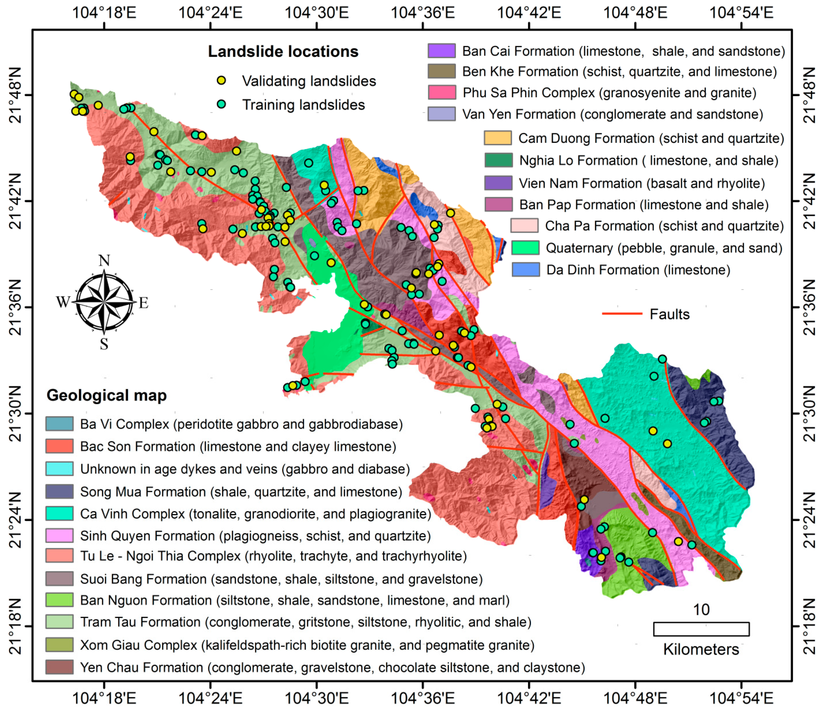
| No | Geological Formations and Complexes | Notation | Area (%) | Landslide Pixels (%) | Thickness (m) |
|---|---|---|---|---|---|
| 1 | Ban Cai Formation | D3bc | 0.76 | 1.18 | 810 |
| 2 | Ban Nguon Formation | D1bn | 3.18 | 2.4 | - |
| 3 | Ban Pap Formation | D1-2bp | 1.61 | 3.0 | 560 |
| 4 | Bac Son Formation | C-Pbs | 4.62 | 1.2 | 360–770 |
| 5 | Ba Vi Complex | U/T1bv | 0.04 | 0 | - |
| 6 | Ben Khe Formation | Є-Obk | 1.23 | 0 | 300–500 |
| 7 | Ca Vinh Complex | G/PP-MPcv | 13.17 | 4.19 | - |
| 8 | Cam Duong Formation | Є1cđ | 4.72 | 4.79 | 500–700 |
| 9 | Nghia Lo Formation | T1-2nl | 0.22 | 6.59 | 500–550 |
| 10 | Phu Sa Phin Complex | sG,Sy/Kpp | 0.42 | 7.18 | - |
| 11 | Quaternary | - | 4.18 | 7.78 | 2–18 |
| 12 | Song Mua Formation | D1sm | 4.01 | 8.98 | 700–800 |
| 13 | Da Dinh Formation | NP-Є1đđ | 0.98 | 0 | 200–400 |
| 14 | Cha Pa Formation | NPcp | 3.07 | 5.39 | 500–700 |
| 15 | Suoi Bang Formation | T3n-rsb | 8.40 | 9.58 | 990 |
| 16 | Tu Le–Ngoi Thia Complex | tR/Ktl–R/Knt | 21.56 | 10.78 | - |
| 17 | Tram Tau Formation | J-Ktt | 15.42 | 10.18 | 200–800 |
| 18 | Unknown in age dykes and veins | - | 0.22 | 11.38 | - |
| 19 | Van Yen Formation | N12vy | 0.04 | 0 | 100 |
| 20 | Vien Nam Formation | T1vn | 0.45 | 0 | 800–1500 |
| 21 | Xom Giau Complex | G/NPxg | 0.25 | 0 | - |
| 22 | Sinh Quyen Formation | PP-MPsq | 9.89 | 8.38 | 1600–1800 |
| 23 | Yen Chau Formation | K2yc | 1.58 | 0 | 300 |
| No. | Parameter | Attribute | Class | Number of Pixels in Class | No. of Landslide in Pixels | % Class Pixels | % Landslide Pixels | FR |
|---|---|---|---|---|---|---|---|---|
| 1 | Slope (o) | 1 | 0–7.92 | 515,596 | 0 | 17.18 | 0 | 0.00 |
| 2 | 7.92–17.82 | 541,470 | 51 | 18.04 | 30.54 | 1.69 | ||
| 3 | 17.82–26.07 | 711,557 | 57 | 23.71 | 34.13 | 1.44 | ||
| 4 | 26.07–34.65 | 668,546 | 42 | 22.27 | 25.15 | 1.13 | ||
| 5 | 34.65–44.88 | 431,726 | 14 | 14.38 | 8.38 | 0.58 | ||
| 6 | 44.88–84.16 | 132,683 | 3 | 4.42 | 1.8 | 0.41 | ||
| 2 | Aspect | 1 | Flat | 143,317 | 0 | 4.77 | 0 | 0.00 |
| 2 | North | 327,283 | 21 | 10.9 | 12.57 | 1.15 | ||
| 3 | Northeast | 418,241 | 26 | 13.93 | 15.57 | 1.12 | ||
| 4 | East | 395,523 | 31 | 13.18 | 18.56 | 1.41 | ||
| 5 | Southeast | 325,218 | 22 | 10.83 | 13.17 | 1.22 | ||
| 6 | South | 339,844 | 24 | 11.32 | 14.37 | 1.27 | ||
| 7 | Southwest | 388,176 | 18 | 12.93 | 10.78 | 0.83 | ||
| 8 | West | 349,264 | 13 | 11.64 | 7.78 | 0.67 | ||
| 9 | Northwest | 314,712 | 12 | 10.48 | 7.19 | 0.69 | ||
| 3 | Elevation (m) | 1 | 0–200 | 311,586 | 11 | 10.38 | 6.59 | 0.63 |
| 2 | 200–400 | 822,680 | 53 | 27.41 | 31.74 | 1.16 | ||
| 3 | 400–600 | 583,190 | 54 | 19.43 | 32.34 | 1.66 | ||
| 4 | 600–800 | 474,387 | 26 | 15.8 | 15.57 | 0.99 | ||
| 5 | 800–1000 | 328,800 | 16 | 10.95 | 9.58 | 0.87 | ||
| 6 | 1000–1200 | 218,799 | 5 | 7.29 | 2.99 | 0.41 | ||
| 7 | 1200–1400 | 122,496 | 2 | 4.08 | 1.2 | 0.29 | ||
| 8 | 1400–1600 | 65,695 | 0 | 2.19 | 0 | 0.00 | ||
| 9 | 1600–1800 | 35,632 | 0 | 1.19 | 0 | 0.00 | ||
| 10 | 1800–2542 | 38,313 | 0 | 1.28 | 0 | 0.00 | ||
| 4 | Curvature | 1 | Concave (<−0.05) | 1,251,973 | 93 | 41.71 | 55.69 | 1.34 |
| 2 | Flat (−0.05–0.05) | 477,452 | 0 | 15.91 | 0 | 0.00 | ||
| 3 | Convex (>0.05) | 1,272,153 | 74 | 42.38 | 44.31 | 1.05 | ||
| 5 | Lithology | 1 | Group A | 1,156,217 | 94 | 38.52 | 56.29 | 1.46 |
| 2 | Group B | 253,577 | 17 | 8.45 | 10.18 | 1.20 | ||
| 3 | Group C | 208,547 | 3 | 6.95 | 1.8 | 0.26 | ||
| 4 | Group D | 335,011 | 18 | 11.16 | 10.78 | 0.97 | ||
| 5 | Group E | 419,594 | 9 | 13.98 | 5.39 | 0.39 | ||
| 6 | Group F | 124,353 | 4 | 4.14 | 2.4 | 0.58 | ||
| 7 | Group G | 504,270 | 22 | 16.8 | 13.17 | 0.78 | ||
| 6 | Slope length (m) | 1 | 0–20 | 917,077 | 36 | 30.55 | 21.56 | 0.71 |
| 2 | 20–50 | 440,296 | 20 | 14.67 | 11.98 | 0.82 | ||
| 3 | 50–100 | 586,102 | 33 | 19.53 | 19.76 | 1.01 | ||
| 4 | 100–150 | 343,241 | 25 | 11.44 | 14.97 | 1.31 | ||
| 5 | 150–200 | 227,146 | 21 | 7.57 | 12.57 | 1.66 | ||
| 6 | 200–2501 | 487,716 | 32 | 16.25 | 19.16 | 1.18 | ||
| 7 | Valley depth (m) | 1 | 0–5 | 1,379,429 | 80 | 45.96 | 47.9 | 1.04 |
| 2 | 5–30 | 538,948 | 34 | 17.96 | 20.36 | 1.13 | ||
| 3 | 30–60 | 320,995 | 16 | 10.69 | 9.58 | 0.90 | ||
| 4 | 60–100 | 272,900 | 10 | 9.09 | 5.99 | 0.66 | ||
| 5 | 100–150 | 221,974 | 20 | 7.4 | 11.98 | 1.62 | ||
| 6 | 150–656 | 267,332 | 7 | 8.91 | 4.19 | 0.47 | ||
| 8 | Distance (Roads) (m) | 1 | 0–100 | 528,102 | 80 | 17.59 | 47.9 | 2.72 |
| 2 | 100–200 | 402,641 | 19 | 13.41 | 11.38 | 0.85 | ||
| 3 | 200–300 | 300,834 | 15 | 10.02 | 8.98 | 0.90 | ||
| 4 | 300–400 | 235,154 | 10 | 7.83 | 5.99 | 0.76 | ||
| 5 | >400 | 1,534,838 | 43 | 51.13 | 25.75 | 0.50 | ||
| 9 | Distance (Rivers) (m) | 1 | 0–100 | 692,491 | 32 | 23.07 | 19.16 | 0.83 |
| 2 | 100–200 | 599,333 | 52 | 19.97 | 31.14 | 1.56 | ||
| 3 | 200–300 | 469,911 | 29 | 15.66 | 17.37 | 1.11 | ||
| 4 | 300–400 | 342,122 | 19 | 11.4 | 11.38 | 1.00 | ||
| 5 | >400 | 897,712 | 35 | 29.91 | 20.96 | 0.70 | ||
| 10 | Distance (Faults) (m) | 1 | 0–250 | 442,100 | 30 | 14.73 | 17.96 | 1.22 |
| 2 | 250–500 | 393,956 | 28 | 13.13 | 16.77 | 1.28 | ||
| 3 | 500–750 | 342,641 | 21 | 11.42 | 12.57 | 1.10 | ||
| 4 | 750–900 | 179,677 | 9 | 5.99 | 5.39 | 0.90 | ||
| 5 | >900 | 1,643,195 | 79 | 54.74 | 47.31 | 0.86 | ||
| 11 | TWI | 1 | 0–8 | 800,751 | 22 | 26.7 | 13.17 | 0.49 |
| 2 | 8–9 | 86,528 | 2 | 2.89 | 1.2 | 0.42 | ||
| 3 | 9–10 | 240,496 | 17 | 8.02 | 10.18 | 1.27 | ||
| 4 | 10–11 | 360,506 | 23 | 12.02 | 13.77 | 1.15 | ||
| 5 | 11–24 | 1,510,529 | 103 | 50.37 | 61.68 | 1.22 | ||
| 12 | TRI | 1 | 0–1 | 366,542 | 0 | 12.21 | 0 | 0.00 |
| 2 | 1–3 | 274,886 | 12 | 9.16 | 7.19 | 0.78 | ||
| 3 | 3–5 | 460,466 | 46 | 15.34 | 27.54 | 1.80 | ||
| 4 | 5–7 | 596,576 | 49 | 19.88 | 29.34 | 1.48 | ||
| 5 | >7 | 1,303,108 | 60 | 43.41 | 35.93 | 0.83 |
| No. | Group | Name | Characteristics of Rock Types |
|---|---|---|---|
| 1 | A | Acid-neutral igneous magmatic rocks | Dacite, felsite, rhyolite, and andesite rocks |
| 2 | B | Terrigenous sedimentary rocks with rich aluminosilicate components | Rhyolites, gritstone, siltstone, carbonates, claystone, alternated dacites, sandstone, and andesite sediments |
| 3 | C | Terrigenous sedimentary and transformative rocks with rich quartz segments | Quartz–mica sandstone, gritstone, sandstone, claystone, siltstone, alternated rhyolites, dacites, carbonates, quartzitic sandstone, andesite sediments, cherty shale |
| 4 | D | Carbonate rocks | Cherty limestone, clayish limestone, and dolomitized limestone |
| 5 | E | Acid-neutral intrusive magmatic rocks | Plagioclase–granite, rhyolite, felsite, dacite, andesite rocks, granophyre, granodiorite, granosyenite, diorite, and quartz-diorite |
| 6 | F | Quaternary deposits | Pluvial and alluvial sedimentary: pebbles, cobble, stone, sand, silt |
| 7 | G | Metamorphic rocks with rich aluminosilicate components | Quartz sericite–schist, quartz mica–schist, quartzite, sericite–quartzite |
© 2019 by the authors. Licensee MDPI, Basel, Switzerland. This article is an open access article distributed under the terms and conditions of the Creative Commons Attribution (CC BY) license (http://creativecommons.org/licenses/by/4.0/).
Share and Cite
Nguyen, V.V.; Pham, B.T.; Vu, B.T.; Prakash, I.; Jha, S.; Shahabi, H.; Shirzadi, A.; Ba, D.N.; Kumar, R.; Chatterjee, J.M.; et al. Hybrid Machine Learning Approaches for Landslide Susceptibility Modeling. Forests 2019, 10, 157. https://0-doi-org.brum.beds.ac.uk/10.3390/f10020157
Nguyen VV, Pham BT, Vu BT, Prakash I, Jha S, Shahabi H, Shirzadi A, Ba DN, Kumar R, Chatterjee JM, et al. Hybrid Machine Learning Approaches for Landslide Susceptibility Modeling. Forests. 2019; 10(2):157. https://0-doi-org.brum.beds.ac.uk/10.3390/f10020157
Chicago/Turabian StyleNguyen, Vu Viet, Binh Thai Pham, Ba Thao Vu, Indra Prakash, Sudan Jha, Himan Shahabi, Ataollah Shirzadi, Dong Nguyen Ba, Raghvendra Kumar, Jyotir Moy Chatterjee, and et al. 2019. "Hybrid Machine Learning Approaches for Landslide Susceptibility Modeling" Forests 10, no. 2: 157. https://0-doi-org.brum.beds.ac.uk/10.3390/f10020157