Article

Insights into the BRT (Boosted Regression Trees) Method in the Study of the Climate-Growth Relationship of Masson Pine in Subtropical China

1
School of Geography, Nanjing Normal University, Nanjing 210023, China
2
School of Resources and Environment, Anqing Normal University, Anqing 246011, China
*
Author to whom correspondence should be addressed.
Submission received: 8 January 2019 / Revised: 27 February 2019 / Accepted: 28 February 2019 / Published: 5 March 2019
(This article belongs to the Special Issue Influence of Climate Change on Tree Growth and Forest Ecosystems)

Abstract

:
Dendroclimatology and dendroecology have entered mainstream dendrochronology research in subtropical and tropical areas. Our study focused on the use of the chronology series of Masson pine (Pinus massoniana Lamb.), the most widely distributed tree species in the subtropical wet monsoon climate regions in China, to understand the tree growth response to ecological and hydroclimatic variability. The boosted regression trees (BRT) model, a nonlinear machine learning method, was used to explore the complex relationship between tree-ring growth and climate factors on a larger spatial scale. The common pattern of an asymptotic growth response to the climate indicated that the climate-growth relationship may be linear until a certain threshold. Once beyond this threshold, tree growth will be insensitive to some climate factors, after which a nonlinear relationship may occur. Spring and autumn climate factors are important controls of tree growth in most study areas. General circulation model (GCM) projections of future climates suggest that warming climates, especially temperatures in excess of those of the optimum growth threshold (as estimated by BRT), will be particularly threatening to the adaptation of Masson pine.

1. Introduction

Tree-ring width (TRW) exhibits a high interannual resolution and has become increasingly important for understanding complex climate systems. In the field of dendroclimatology, the development of climate-sensitive chronologies of subtropical and tropical areas remains an important issue. Therefore, studies involving detailed climate-growth analyses in warm and humid subtropical regions of China have been developed in recent decades [1,2,3,4,5,6,7,8,9,10,11,12,13,14]. Despite these achievements, additional studies on the undeniable problems in this area are still necessary. Masson pine (Pinus massoniana Lamb.), one of the most widely distributed tree species in the subtropical regions of China, has high environmental and social impacts. This species grows as well in the lowlands as it does in the highlands and occurs at altitudes ranging from a few meters to approximately 2000 m above sea level (a.s.l.). Because of this, this species occurs in highly varying climatological conditions, ranging from moist lowland river valleys to the dry mountain plateaus in the interior parts of China [15]. Thus, Masson pine is an ideal tree species for subtropical tree-climate research in China. However, using tree rings for dendroclimatology studies in tropical and subtropical areas is often complicated, and the responses of trees to the climate variables can be nonlinear and can even vary across species and ecosystems [16,17]. With respect to the Masson pine, previous ecophysiological or climatological studies have shown that the climate-growth relationship may exhibit complex patterns. For example, Kuang et al. [1] reported that both temperature and precipitation are significantly linearly related to tree growth. Duan et al. [5] showed that only the January–April average temperature was significantly related to growth. Chen et al. [4] reported a significant negative correlation between growth and the August–October average temperature. Xia et al. [6] reported a significant negative correlation between TRW and May–August average temperature during the growing season. However, some authors reported a significant nonlinear relationship between these two factors. [18,19]. With respect to the majority of dendroclimatological studies, only important climate variables and the tree-growth relationship are well understood, and reliable climate reconstruction works can be implemented [20]. Traditionally, a common practice in dendroclimatology is to correlate TRW with monthly or seasonal climate data in a linear form [21]. However, the tree ring records are likely to be nonlinear biophysical processes and may be complicated [14,21,22,23,24,25,26]. Therefore, an increasing number of authors have acknowledged nonlinearities in the climate-growth system [17,27,28,29,30,31]. One of the current methods used for calibrating the nonlinear climate-growth relationship is the Vaganov–Shashkin (VS) model [23,32,33,34,35]. However, this performs worst in warm and wet environments [22]. Thus, given that our study occurred in a subtropical area, our focus turned to using machine learning methods. Artificial neural network (ANN) was considered as a better choice for careful assessment of complex climate-growth relationships [20,36,37,38,39,40,41,42,43,44,45,46,47,48,49,50]. However, the learning method process of an ANN is a “black box operation” [51,52,53], meaning that it is sensitive to overfitting and ANNs have difficulty evaluating the contribution of each variable to the results, from a statistical point of view [53,54]. An ensemble machine learning method (i.e., a boosted regression trees (BRT)), developed by Friedman [55], appears to be a promising method for detecting nonlinear relationships, as demonstrated by some recent studies that aimed to model tree growth responses to climate [51,56,57,58]. To the best of our knowledge, this technique has not been applied in dendroclimatic studies with respect to complex interactions in dendroclimatic relationships in subtropical China. Thus, this paper attempts to examine the application of the BRT for (1) Selecting the relatively important climate predictors for TRW, (2) investigating the complex climate-growth relationship, and (3) evaluating the potential thresholds concerning the effects of climate variables and estimate the influence of the warming climate on the growth of Masson pine.

2. Materials and Methods

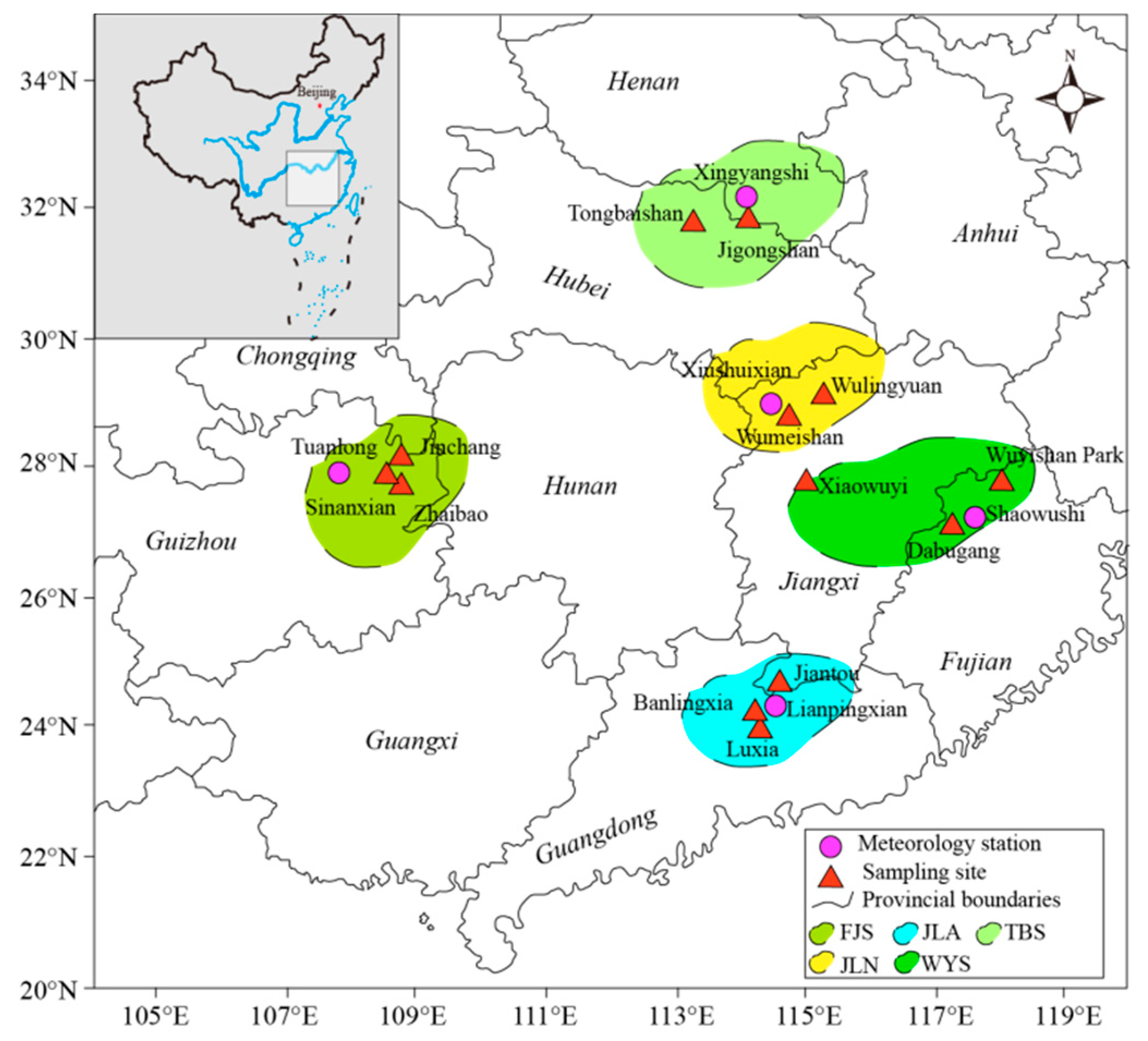
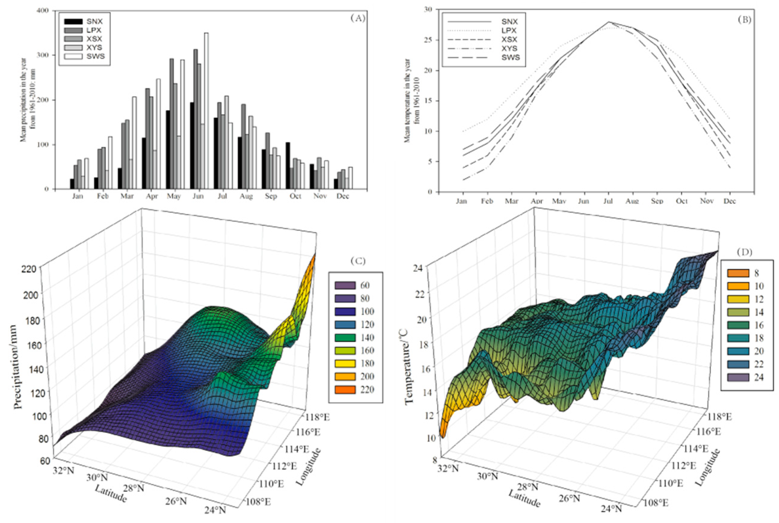
2.1. Geography and Climatology of the Study Areas

Tree-ring records from individual sites can also reflect the influence of unobserved localized and nonclimatic influences [21,59]. To systematically explore the relationship between Masson pine and climate on a large spatial scale, we collected tree ring data from five areas, that were subjected to little human disturbance (Table 1).
Fanjing Mountain (FJS), located in the western portion of the Masson pine-dominated area, contains vegetation associated with typical subtropical evergreen broad-leaved forest zonal primitive forest vegetation. The annual average temperature is approximately 17.4 °C. The lowest temperature is approximately 6.1 °C in January, and the highest temperature is approximately 27.8 °C in July. The annual average precipitation is approximately 1129.5 mm, and the average relative humidity is approximately 74%. Three sampling sites were selected here: Tuanlong, Jinchang and Zhaibao.
The southern sampling area was Jiulian Mountain (JLA), known as the “gene bank of biological resources”, located at the border of the Jiangxi province and Guangdong province. Masson pine trees in this area composes secondary forest. The annual average temperature is approximately 16.4 °C, the lowest temperature in January is approximately 6.8 °C, and the highest temperature is in July, is approximately 24.4 °C. The average annual precipitation is approximately 2155.6 mm, and the average annual relative humidity is approximately 85%. The sampling sites here include Jiantou, Banlingxia and Luxia.
Near the center of the Masson pine distribution, we chose to sample on Jiuling Mountain (JLN), which is the site of the original Masson pine forest. The annual average temperature is approximately 16.7 °C, the lowest temperature in January is approximately 4.4 °C, and the highest temperature in July is approximately 28.2 °C. The annual average precipitation is approximately 1653 mm, and the average relative humidity is approximately 79%. The rainfall is abundant during every season each year, and the climate is warm. The two sampling sites in this area are Wulingyan and Wumeishan.
The fourth sampling area, located at the northern margin of the Masson pine distribution, is Tongbai Mountain (TBS), which is dominated by its primary forest. The highest altitude of the Tongbai Mountain is 1140 m and the climate of the north subtropical region is considered monsoon is humid. The average annual temperature is approximately 15 °C, the average temperature in January is approximately 2 °C, and the average temperature in July is approximately 28 °C. The climate is mild and sunshine is abundant. The northern region lacks an alpine barrier, and the cold wave from the north can continue into winter. The winter temperature is low, the annual precipitation is approximately 1168 mm, and the annual average relative humidity is approximately 74%. Tongbaishan and Jigongshan were the two sampling sites.
We also developed TRW chronologies on Wuyi Mountain (WYS), which is covered with both natural and artificial secondary forests. The annual average temperature is approximately 18 °C, the lowest temperature in January is approximately 7.1 °C, and the highest temperature in July is approximately 27.8 °C. The average annual precipitation is approximately 1818.6 mm, and the average relative humidity is approximately 81%. The sample area here mainly includes mainly three sampling sites: Xiaowuyi, Wuyishan Park and Dabugang.

2.2. Tree-Ring Preparation and Measurement

The sampling sites were selected on the south slope, far away from human residents. The average slope was approximately 20 to 35 degrees. There were 2 to 3 sampling subsites in each area. There was no evidence indicating that natural conditions such as soil and water supply had experienced extreme disturbance at each sampling site. According to the sampling standards for the International Tree-Ring Data Bank (ITRDB), a tree-ring core with a diameter of 5.15 mm of Masson pine was drilled on both sides of the tree stem, which were parallel to the direction of the slope. In total, 207 old and dominant tapped trees were selected to maximize the temporal extent of the TRW records. Tree ring cores were preserved in a paper tube and then returned to the laboratory. After drying in a natural state, the tree-ring cores were fixed and sanded with increasingly finer sandpaper, up to 400 grit, to produce visible rings [60]. The skeleton plot was first used to validate the dating, after which the pseudo and missing tree-rings were initially identified [21]. The preliminary calendar age for each tree ring was determined. Afterward, the ring width was measured using an AcuRite (VoorTech, New York, NY, USA) measuring system, with an precision of 0.001 mm. Finally, the COFECHA program was used to check and control the quality of cross-dating, and samples with week correlation, large singularities and juvenile effects were rejected [61,62]. The ARSTAN program was used to establish chronologies [63]. After cross-dating, the chronologies were subjected to detrending and other statistical procedures were used routinely on the tree-rings [21]. We applied the cubic spline curve (SP), which eliminates low-frequency variations and enhances high-frequency climate signals [64]. The resulting population chronology is often described with various statistical measures to quantify the signal to noise ratio (SNR) [65], the mean sensitivity (MSX) [66,67], standard deviation (SD), the commonly used expressed population signal (EPS) [68], with a threshold of 0.85 [69], explained variance in first eigenvector (PC1) and the Gini coefficient [70,71]. In addition, principal component analysis was used to estimate the common similar and different regional environments that influenced the growth process of the trees. These statistical analyses (Table 2) were performed via R (version 3.5.1), using the dplR package [72,73,74].

2.3. Climate Data

Climate data were used for detecting dendroclimatology from the CRUTS 4.01 datasets (https://crudata.uea.ac.uk/cru/data/hrg/) [75]. Meteorological station records were obtained from the National Meteorological Information Center (http://data.cma.cn/). The locations of the five homogenized meteorological stations are as follows: the Sinanxian (SNX) station is close to FJS, the Lianpingxian (LPX) station is near JLA, the Xiushuixian (XSX) station is a short distance away from JLN, the closest station to TBS is in Xinyangshi (XYS), and the Shaowushi (SWS) station is near WYS. Basic climate information is shown in Figure 1 and Figure 2. In Figure 2A,B, both precipitation and temperature display a single peak that essentially belongs to the climate type of the same period of rain and heat. The peak precipitation occurs each year in June, while the peak surface temperature occurs in July; spring, autumn and winter are relatively dry. The precipitation data from the meteorological stations indicate that the annual precipitation in the TBS sampling area is the lowest, and that in the WYS sampling area is the highest. The temperature records from the meteorological stations indicate that the temperature of the TBS sampling area is relatively low, and that of the JLA sampling area is relatively high. Based on the CRUTS 4.01 datasets and instrumental data, the annual temperature and precipitation gradually decreases from southeast to northwest (Figure 2C,D) in our analysis area, and their difference are quite obvious. When viewed alongside the latitude, the precipitation along the western margin of the Masson pine distribution changes little, but the gradient is obvious along the eastern margin. Therefore, the hydroclimatic environment of Masson pine differs in the subtropical wet monsoon climate, where heat is abundant and precipitation is plentiful.

2.4. BRT Methods

The generalized boosting model (GBM) has the ability to characterize nonlinear changes. Elith et al. [76] produced a detailed paper concerning the applications of a boosted regression trees (BRT) method under the (GBM) framework in relation to ecological data. The strengths of the GBM model (including BRT) were threefold: (1) It facilitated the processing of multiple interactive variables; (2) characterized partial dependence, i.e., potential nonlinear and nonmonotonic changes in response functions; and (3) had a high predictive accuracy and abundant flexibility. BRT models are robust in relation to small-size or absent data [77]. In this paper, BRT models were implemented using the GBM package (version 2.1.4) [76,78].
The first consideration of BRT models is distribution. For continuous predictors, the Gaussian distribution is selected (to minimize the squared error), which provides a better correlation between the observed value and the GBM model estimate [56,78]. We took the train function in the caret package to explore the optimal values for the foremost parameters [79]. The function tries a number of different parameters, compares the error rates, and then suggests the smallest parameter that generates an appreciable decrease in the error rate. The first two parameters generated were shrinkage (learning rates) and the number of trees (nt). A good rule of thumb for an ideal shrinkage value is 0.001, which is close to the point of diminishing return. Shrinkage is also related to the number of trees. The optimal number of trees (minimizing the prediction bias) was estimated using 10-fold cross-validation [51,76]. To increase the model accuracy, randomness is included using a bagging fraction of 0.5 [76].
The expected sensitivity of the tree growth to the climate variables is quantified based on two factors: the relative influence of the variables and the partial dependence plots [56]. With respect to the BRT models, an extension of a variable’s “relative influence” (here, the relative influence refers to the contribution of each variable to the minimization of the loss function) was developed by Friedman [55]. The relative importance is calculated by averaging the number of times a variable is selected for splitting, weighted by the squared improvement to the BRT model, as a result of each split, it is then scaled so the values sum to 100. Variables whose relative influence exceeds the median of each model are classified as “highly important”, and those below the median are classified as having “low importance” [56]. The partial dependence plots indicate the relationship of the predictor variable “X” with the response variable “Y”, as well as the former’s dependence on the latter. In current applications, a change in the quantitative tree growth index of partial dependence plots is quantified as a function of the season climate signal.
In southeastern China, the growth season of coniferous tress generally occurs from early April to November [80]. Cai and Liu [81] selected the March–October season length for Pinus taiwanensis Hayata. Zhang et al. [82] accurately quantified the length of the growing season of Masson pine. These authors have shown that December is the beginning of the dormancy period of Masson pine. The cambium is inactive in January and is likely to be semidormant. February is the end of the dormancy period of the Masson pine or the beginning of its germination, and buds appear in March (i.e., the beginning of rapid growth). Hardly any growth occurs in the summer, after which rapid growth begins again. Therefore, in terms of tree physiology relevant to studying the dendroclimatic relationships, the Masson pine growth season selected in this study is listed in Table 3. To avoid overfitting, we used the “vif” function in the car package (version 3.0-2) [79], to exclude any collinearity variables (vif >5). We found that the selected climate variables were not collinear.

3. Results

3.1. Tree Ring Chronology Statistics

By the use of COFECHA quality test, which included several trials of different frequency responses and wavelength cutoff years, the standard and residual chronologies of the TRW in five study areas were ultimately established with an SP (a 50% frequency response and wavelength cutoff at 30 years) (Figure 3). The chronology statistics of each tree ring chronology series indicate that the chronology can be used for subsequent analyses (Table 2). The high mean sensitivity obtained (0.208–0.256) is greater than 0.2. The mean sensitivity is approximately 0.2, which is generally accepted as a series that is sensitive enough for climate reconstruction [83]. The first autocorrelation value for the raw width series of this study ranged from 0.587 to 0.689. The mean Gini coefficient shows that it satisfies three hypotheses related to variability in the ring-width increment: (1) it would decrease as the latitude increased; (2) it would increase with the longitude (i.e., west to east); and (3) it would decrease as elevation increased [70]. EPS values ranged from 0.931 to 0.970, indicating that each chronology was dominated by a coherent stand-level signal. The series intercorrelation, SNR, PC1, and EPS of the same sample area were all relatively high, which indicated that the variation in the ring width of each sequence at the same sampling site was synchronized, indicating that they might be affected by consistent changes in the external climate and environment.
As shown in Figure 4, the cumulative proportion of the first three principal components is as high as 83.1%, the value of PC1 is 40.01%, and the other three principal components are also higher than 10%. The loadings of JLA, WYS and JLN are relatively large in the first principal component, while they are relatively small for TBS and FJS. On the other hand, the loadings of FJS, TBS and JLN are relatively large in the second principal component. These results show that the regional climate conditions affecting the growth of Masson pine may be relatively consistent, and that niche factors have an impact on tree growth.

3.2. Performance of the BRT Models

To evaluate the performance of the BRT model, resampling and cross-validation were used [84]. With respect to the regression of continuous data, the mean absolute error (MAE) and the root mean squared error (RMSE) are easy to understand and are widely used to measure the performance of machine learning problems. If these values are small, then the models can make accurate predictions when faced with “new” data [85]. The R-squared values (R2) for the BRT model ultimately applied across all five study areas are 0.491 (FJS), 0.559 (JLA), 0.608 (JLN), 0.597 (TBS), and 0.569 (WYS). The BRT model performs better for TBS and JLN than for the other areas. In addition, we compared it with other models, including the generalized linear model (GLM), random forests (RF), and bayesian regularization neural network (BRNN) models (Figure 5). The RMSE and MAE values among the four models are relatively small in the five study areas and give slightly more accurate results. However, the nonlinear models (BRT, BRNN and RF) slightly outperform the linear model. These results show that the BRT model can be a useful tool for dendroclimatic studies.

3.3. Relative Influence of Seasonal Climate Factors

One major advantage of BRT models is that they can select variables of relative importance. By ranking climate predictors based on how much they influence TRW, the values of relative influence from the five study areas can be determined (Table 3 and Figure 6). Some aspects of the growth response to climate were relatively consistent across all five study areas. The September–November precipitation and February–May temperature have a comparatively large influence on tree growth in the five study areas, and spring temperatures tended to be more influential than summer temperatures. Despite these similarities, some differences occurred between the study areas. For example, winter temperatures were generally unimportant, except at JLA, where the December–January temperature has a relatively strong effect on growth. The June–August temperature was relatively important at JLA and JLN, but less important at FJS, TBS and WYS.

3.4. Nonlinearity of the Data

A frequency distribution, which is a statistical tool, was generated to visualize the distribution of one seasonal climate variable (Figure 7). The interannual variations of climatic conditions in the five study areas are quite different, and extreme climate phenomena occurred in some years. For example, at WYS, for the prior September–November precipitation variable, the chart shows a skewed frequency distribution, with variation ranging from 35 to 150 mm; moreover, the frequency in some years is high, whereas that in others is low, but there is a high probability of a higher frequency or concentration of 60 mm. Combining partial dependence plots and climate annual dynamics will help elucidate these complex climate–growth relationships. We found that with changes in climatic conditions, the sensitivity of growth to climatic conditions will increase or decrease rapidly. Afterward, the partial dependence curve eventually flattens. When the partial dependence curve was associated with fluctuation, there was a general asymptotic growth response model, i.e., tree growth is relatively insensitive to a wide range of climatic conditions [56]. Therefore, the asymptotic growth response to climate is highly common in the study areas.
The upper-right plots of Figure 7 show that the February–May temperature is somewhat directly related to the tree growth at FJS. The interannual variations of the February–May temperature range from 10 to 13.3 °C and center on 11–12 °C. The partial dependence plots of FJS on February–May temperature show that, at 11 °C, the value is 0.92, after which there is an upward trend followed by the peak (0.95). Tree growth was relatively insensitive to the colder years, but during the warmer years, the sensitivity of tree ring growth to the temperature of the time period increased rapidly. Note that February is the beginning of the germination of Masson pine. At this time, low temperatures may slow the germination process and delay growth.
Residual plots are a useful graphical tool for identifying nonlinearity. The presence of a pattern may indicate a problem with some aspects of a linear model. Figure 8 displays a residual plot from the linear regression. The residuals exhibit obvious trends in some study areas, which may indicate nonlinearity of the data. For example, an upward growth trend in the bottom-right panel of Figure 8 shows that the relationship between tree growth and the September–November precipitation of the previous year may be nonlinear at WYS.

3.5. Threshold of Climate-Growth in the Future

To assess the potential impact of future climate change on tree growth, we estimated the optimal seasonal temperature or precipitation range of seasons for tree growth. These optimal thresholds were defined within the partial dependency plots derived by the BRT model [56]. These optimal growth ranges are then compared with the mean distribution of the climatic values of the seasons in the CMIP5 datasets for the period of 2006–2100 (https://esgf-node.llnl.gov/projects/cmip5/). A comparison of the CMIP3 and CMIP5 datasets gave a slightly more accurate result for simulating future climate change in China [86]. Through comparison with the CRUTS 4.01 datasets, we can quantify the sensitivity of tree growth to future climate change and determine what variables will lead to significant changes in Masson pine, i.e., relative optimal growth hydroclimate conditions (Figure 9 and Figure 10). Understanding how climate change will affect the cambial growth of Masson pine in the future is of practical significance.
The average temperature in the next 100 years will be higher than that of the historical datasets (Figure 9). The box chart shows that the median values of the seasonal temperature of the CMIP5 datasets are higher than the optimum growth temperature, as estimated by the BRT models. These temperatures correspond to the relatively cool temperature values to be experienced for the next 100 years at most sites and suggest that the optimum conditions for growth here have been relatively rare. It can be seen that the median temperature of each season during the 1901–2016 period is essentially no more than that of the optimum growth temperature, but in some years, the temperature exceeds the optimum temperature threshold. These years, which exceed the optimum growth temperature, may strongly influence on the growth of Masson pine. In some study areas, there are abnormal temperature occurrences in some years, i.e., the abnormally low June–August temperature at JLA and the abnormally high February–May temperature at TBS.
Generally, the optimum precipitation range suitable for Masson pine growth varied substantially among the study areas (Figure 10). The median values of seasonal precipitation during the next 100 years were essentially equal to those within the CRUTS 4.01 datasets. Even some seasonal precipitation is lower than the historical precipitation data. For example, at JLA, the future median February–May precipitation is 101 mm, but the historical median value is 194 mm. The interannual June–August precipitation (regardless of the current year or prior year) varies greatly in the five study areas. Moreover, the interannual February–May precipitation variations are relatively large. In different areas, the threshold of precipitation, suitable for tree growth in different seasons, is very different, and the relative influence of different climatic variables varies from place to place. These differences are not explained by the location of the study area or its topography, and the reasons for this nonuniformity deserve further study.

4. Discussion

4.1. BRT as a Potential Tool for Analysing Climate-Growth Relationships

Linear regression (correlation analysis, multiple regression, principal component regression, etc.) is commonly used to analyze the statistical relationship between the TRW (as a proxy) and climate data [21,87]. Pearson’s product-moment correlation has become a workhorse for analyzing complex dendroclimatic relationships. However, Pearson’s coefficient is very sensitive to outliers; even a single outlier can change the direction of the coefficient. Additionally, this technique cannot capture the nonlinear relationship between two variables. Because the BRT model is insensitive to outliers and multicollinearity, it can fit complex nonlinear relationships and can automatically handle the interactive effects between predictors [76,77,88]. We preliminarily used this technique to determine the most important variables, evaluate potential thresholds regarding the effects of these climate variables, and examine their functional responses. Based on two evaluation metrics (RMSE and MAE), our analyses confirmed the results of a previous study showing that the BRT, BRNN and RF models performed better than the generalized linear models (GLMs) did [45,89,90], with less variance and bias. Moreover, the BRT model performed better for TBS and JLN than for the other areas. Considering the ecological and climate factors, both TBS and JLN are dominated by primeval Masson pine forest, and the highest temperature in July is higher than 28 °C. On the other hand, in conjunction with WYS, a lower altitude may be another factor that affects the performance of BRT methods. However, this result deserves further study. To our knowledge, some studies have shown that there are nonlinear climate-growth relationships in subtropical areas of China [18,19,43,91]. Thus, it is necessary to further explore this issue.
The frequency distribution of the historical climate data shows that some outliers occur during some seasons of different years. This phenomenon indicates that extreme climate records are also frequent in subtropical regions [92], which would cause a divergent problem and a nonlinear response pattern [43,91,93].
In addition, the residual plots exhibit obvious trends in some study areas, which may provide an indication of nonlinearity of the data [94]. We assessed the partial dependence plots and found that the asymptotic growth response to climate was relatively common in the Masson pine growth models. We speculated that this pattern of an asymptotic climate-growth relationship may exhibit nonlinear patterns [56,95]. Until a certain threshold, the climate-growth relationship may be linear. Once beyond this threshold, tree growth will be insensitive to some climate factors, after which a nonlinear relationship may occur. Some authors have stated that the growth of Pinus taiwanensis exhibits some nonlinear characteristics associated with temperature and precipitation, and the linear relationship only holds true within a certain threshold of subtropical China [91]. The widespread occurrence of growth thresholds indicates that small climate changes may have great impacts on the growth of Masson pine. In fact, tree growth is a continuously dynamic process. While tree-ring datasets provide insight into a limited interval of climate conditions, the long-term impact of tree growth on the ontogenetics of Masson pine remains unknown. The assumption that the dendroclimatic relationship is constant across the whole spectrum of climate-growth responses in linear regression is not always correct [22,46]. The response of tree growth to climate is a complex process and there may be interactive and compensatory effects between climate variables in different seasons and years, which makes for an unstable relationship between tree growth and climate [37,91].
Last, factor–discrete can be used to explain the nonlinearities in physiological responses to climate [56,95]. Discrete climate factors are revealed in cases where the response threshold is relatively consistent among study areas. In our studies, thresholds in tree responses to the February to May temperature were reached from 11 to 18 °C in the majority of our study areas. The temperature thresholds of Masson pine in the early part of the growing season are similar to those in some previous studies [96,97]. Therefore, this phenomenon probably represents a real physiological threshold in the growth response to temperature.
The enhanced regression model (BRT) allows us to clearly identify the threshold of the climate-growth response and develop a statistical model of that response, and this model has a greater explanatory power than does the linear statistical model. The universality of nonlinear responses to climate is important for understanding how trees respond to climate variability in subtropical China, and our ability to identify and describe these threshold responses is crucial for developing accurate predictions of the impact of climate warming on subtropical forests.

4.2. Seasonal Features in Growth-Climate Relationships

Our relative influence analysis using the BRT technique showed that the response patterns of Masson pine to climate change exhibit both similarities and differences. The beginning of each phenology of Masson pine coincides with the month of the temperature variable that affects the growth of the species, as revealed by the BRT model. Principal component analysis reveals that the regional environment affecting the growth of Masson pine was relatively consistent, but the niche factors impact the growth of trees.
Notably, with the exception of wet areas with relatively low elevation (JLA and WYS), the February–May temperature significantly impacts Masson pine growth. In addition, the growth of Masson pine in wet areas at high elevation was affected by the temperature in February [98]. In warm-temperate forests, stem radial growth at the beginning of growing seasons is generally limited by temperature [99,100]. Our similar results at JLN confirm previous findings in which, compared with other seasons, the January–April temperature has a greater impact on the growth of Masson pine in Hunan and Jiangxi provinces [5]. Other dendroclimatological studies in southeastern China have confirmed that temperatures during the spring and early summer strongly influence coniferous forests [101,102]. With respect to northern region of the Masson pine distribution zone, growth is related to the squares of the temperature during February, May and August [18,19]. In fact, in our northern study area (TBS), the February–May temperature had an important influence on the growth of Masson pine. The increase of the temperature in the spring is conducive to the division and growth of early wood cells, and early wood is the main component of radial tree growth.
Under normal climatic conditions, growth at an altitude of 300 m was affected by the mean monthly precipitation during the previous October [98]. In Fujian Province, the autumn and winter temperature and precipitation are highly important for width of tree-rings [4,8,103,104], at WYS (mean altitude of 275 m a.s.l.), that the September–November temperature and previous September–November precipitation yield the greatest relative importance value. In the southern distribution region of Masson pine (JLA), the tree growth is highly sensitive to the winter temperature and autumn precipitation. These results are consistent with those of a previous study that showed that the winter temperature negatively affects on tree growth [103]. Compared with the findings in a previous study in the tropical area [17], our findings showed that the September–November precipitation is a growth-limiting factor at JLA. In addition, the September–November precipitation of the current years is important for tree growth at TBS and JLN. In the Lushan Mountains, near to our study area (JLN), the precipitation during the dry season (July–November) greatly promoted stem growth [105]. In the northern region of the distribution zone of Masson pine, the August–November precipitation positively affected on tree growth [18].
Consequently, the relatively important climate factors do vary across the whole distribution range of Masson pine, but the spring and autumn climate conditions mainly affect tree growth. These results may explain the bimodal radial growth pattern of Masson pine stems, as two growth peaks during the transitional seasons (spring–early summer and autumn) and a decreased growth rate in the summer were observed [105]. Zhang et al. [82] also mentioned that the growth of Masson pine during dry seasons is obviously stronger than during the wet seasons.

4.3. Influence of Global Warming

We briefly considered the possible impacts of future climate change on the growth of Masson pine tree-rings based on general circulation model (GCM) projections. In the context of future climate change, subtropical monsoon climate will be characterized by milder winters and hotter summers. When the CMIP5 datasets were compared, the optimum growth temperature occurred within a relatively low range. These findings suggest that warming during the next 100 years is likely to lead to significant changes in Masson pine. Temperatures exceeding the thermal optimum for growth will reduce net photosynthesis due to increased photorespiration [106,107]. In addition, based on the CMPI5 datasets, future precipitation during the season from September–November will dip below the optimum precipitation threshold. In the future, the growth of Masson pine may not benefit from future global warming and will exhibit increased sensitivity to conditions of the dry season (September–November).
Trees growing at temperatures higher than those for the optimum growth conditions tend to distribute less biomass to their roots [93]. This phenomenon could lead to a decrease in or a movement of Masson pine. Some authors have confirmed that the declining trend and the distribution area of Masson pine will likely gradually shift northward with the warming climate [82,103]. Thus, the hydrological combination during the dry season will play an important role in the normal growth of Masson pine indicating that the growth of this species will be affected not only by environmental factors (temperature and precipitation) but also by net photosynthetic energy.

5. Conclusions

In this paper, climate-growth correlation analyses were carried out on a large spatial scale, based on the tree-ring chronologies of Masson pine. Compared with the results of previous studies, our results showed that, by the use of a nonlinear machine learning algorithm (a BRT model), spring and autumn conditions were relatively highly influential on Masson pine. GCM projections of the future climate suggest that the warming climate, especially temperatures in excess of those of the optimum growth threshold (as estimated by BRT), will be particularly threatening to the adaptation of Masson pine. The relationship between the Masson pine TRW and climate is unstable when the habitat exceeds the optimal threshold value and may be nonlinear. The BRT method can be a variable selection tool for identifying the important linear and/or nonlinear independent climate variables, which can then be used in more classic predictive models.

Author Contributions

Conceptualization, J.W.; Data curation, L.M.; Investigation, Z.S. and Q.Z.; Writing—original draft, H.G.; Writing—review and editing, H.G.

Funding

This work was supported by the National Natural Science Foundation of China (grant No. 41271204), and the Social Science Foundation of Anhui, China (grant No. SK2016A0544).

Acknowledgments

We are grateful for the helpful and constructive comments of three anonymous reviewers. We also thank the assistant editor (MS Winter Wang) for her help.

Conflicts of Interest

The authors declare no conflict of interest.

References

  1. Kuang, Y.W.; Sun, F.F.; Wen, D.Z.; Zhou, G.Y.; Zhao, P. Tree-ring growth patterns of Masson pine (Pinus massoniana L.) during the recent decades in the acidification Pearl River Delta of China. For. Ecol. Manag. 2008, 255, 3534–3540. [Google Scholar] [CrossRef]
  2. Sun, F.; Kuang, Y.; Wen, D.; Xu, Z.; Li, J.; Zuo, W.; Hou, E. Long-Term Tree Growth Rate, Water Use Efficiency, and Tree Ring Nitrogen Isotope Composition of Pinus massoniana L. in Response to Global Climate Change and Local Nitrogen Deposition in Southern China. J. Soils Sediments 2010, 10, 1453–1465. [Google Scholar] [CrossRef]
  3. Kuang, Y.; Zhou, G.; Wen, D.; Li, J.; Sun, F. Analysis of Polycyclic Aromatic Hydrocarbons in Tree-Rings of Masson Pine (Pinus massoniana L.) from Two Industrial Sites in the Pearl River Delta, South China. J. Environ. Monit. 2011, 13, 2630–2637. [Google Scholar] [CrossRef] [PubMed]
  4. Chen, F.; Yuan, Y.; Wei, W.; Yu, S.; Zhang, T. Reconstructed Temperature for Yong’an, Fujian, Southeast China: Linkages to the Pacific Ocean Climate Variability. Glob. Planet. Chang. 2012, 86–87, 11–19. [Google Scholar] [CrossRef]
  5. Duan, J.; Zhang, Q.-B.; Lv, L.; Zhang, C. Regional-Scale Winter-Spring Temperature Variability and Chilling Damage Dynamics over the Past Two Centuries in Southeastern China. Clim. Dyn. 2012, 39, 919–928. [Google Scholar] [CrossRef]
  6. Xia, P.; Yin, S.; Jiang, J. Pinus aiwanensis Tree-Ring Chronology and Its Response to Climate. Procedia Environ. Sci. 2012, 13, 307–315. [Google Scholar] [CrossRef]
  7. Zheng, Y.; Zhang, Y.; Shao, X.; Yin, Z.-Y.; Zhang, J. Temperature Variability Inferred from Tree-Ring Widths in the Dabie Mountains of Subtropical Central China. Trees 2012, 26, 1887–1894. [Google Scholar] [CrossRef]
  8. Chen, F.; Yuan, Y.; Yu, S.; Zhang, T. Influence of Climate Warming and Resin Collection on the Growth of Masson Pine (Pinus massoniana) in a Subtropical Forest, Southern China. Trees 2015, 29, 1423–1430. [Google Scholar] [CrossRef]
  9. Li, D.; Fang, K.; Li, Y.; Chen, D.; Liu, X.; Dong, Z.; Zhou, F.; Guo, G.; Shi, F.; Xu, C.; et al. Climate, Intrinsic Water-Use Efficiency and Tree Growth over the Past 150 Years in Humid Subtropical China. PLoS ONE 2017, 12, e0172045. [Google Scholar] [CrossRef] [PubMed]
  10. Liu, Y.; Ta, W.; Li, Q.; Song, H.; Sun, C.; Cai, Q.; Liu, H.; Wang, L.; Hu, S.; Sun, J.; et al. Tree-Ring Stable Carbon Isotope-Based April–June Relative Humidity Reconstruction since Ad 1648 in Mt. Tianmu, China. Clim. Dyn. 2018, 50, 1733–1745. [Google Scholar] [CrossRef]
  11. Zhao, Y.; Shi, J.; Shi, S.; Wang, B.; Yu, J. Summer Climate Implications of Tree-Ring Latewood Width: A Case Study of Tsuga longibracteata in South China. Asian Geogr. 2017, 34, 131–146. [Google Scholar] [CrossRef]
  12. Williams, R. The Effects of Resin Tapping on the Radial Growth of Masson Pine Trees in South China-A Case Study. Agric. Res. Technol. Open Access J. 2017, 8. [Google Scholar] [CrossRef]
  13. Zhao, Y.; Shi, J.; Shi, S.; Yu, J.; Lu, H. Tree-Ring Latewood Width Based July–August SPEI Reconstruction in South China since 1888 and Its Possible Connection with ENSO. J. Meteorol. Res. 2017, 31, 39–48. [Google Scholar] [CrossRef]
  14. Acevedo, W.; Fallah, B.; Reich, S.; Cubasch, U. Assimilation of Pseudo-Tree-Ring-Width Observations into an Atmospheric General Circulation Model. Clim. Past 2017, 13, 545–557. [Google Scholar] [CrossRef]
  15. Farjon, A. Pinus Massoniana. The IUCN Red List of Threatened Species 2013: E.T42379A2976356. Available online: https://0-doi-org.brum.beds.ac.uk/10.2305/IUCN.UK.2013-1.RLTS.T42379A2976356.en (accessed on 28 February 2019).
  16. Brienen, R.J.W.; Schöngart, J.; Zuidema, P.A. Tree Rings in the Tropics: Insights into the Ecology and Climate Sensitivity of Tropical Trees. In Tropical Tree Physiology; Goldstein, G., Santiago, L.S., Eds.; Springer International Publishing: Cham, Germany, 2016; Volume 6, pp. 439–461. [Google Scholar]
  17. Anhuf, D.; Schleser, G.H. Tree Ring Studies in the Tropics and Subtropics. Erdkunde 2017, 71, 1–4. [Google Scholar] [CrossRef]
  18. Xia, B.; Lan, T.; He, S. Nonelinear Response Function of Growth of Pinus massoniana to Climate. Chin. J. Acta Phytoecol. Sin. 1996, 20, 51–56. [Google Scholar]
  19. Lan, T.; Xia, B.; He, S. Tree ring Analysis on Relation of Pinus massoniana Growth to Climate Factors. Chin. J. Appl. Ecol. 1994, 5, 422–424. [Google Scholar]
  20. Jevšenak, J.; Levanič, T. Should Artificial Neural Networks Replace Linear Models in Tree Ring Based Climate Reconstructions? Dendrochronologia 2016, 40, 102–109. [Google Scholar] [CrossRef]
  21. Fritts, H.C. Tree Rings and Climate; Academic Press: London, UK; New York, NY, USA; San Francisco, CA, USA, 1976. [Google Scholar]
  22. Evans, M.N.; Reichert, B.K.; Kaplan, A.; Anchukaitis, K.J.; Vaganov, E.A.; Hughes, M.K.; Cane, M.A. A Forward Modeling Approach to Paleoclimatic Interpretation of Tree-Ring Data. J. Geophys. Res. 2006, 111. [Google Scholar] [CrossRef]
  23. Vaganov, E.A.; Hughes, M.K.; Šaškin, A.V. Growth Dynamics of Conifer Tree Rings: Images of Past and Future Environments; Springer: Berlin, Germany, 2006. [Google Scholar]
  24. Andreuhayles, L.; D’Arrigo, R.; Anchukaitis, K.J.; Beck, P.S.A.; Frank, D.; Goetz, S. Varying Boreal Forest Response to Arctic Environmental Change at the Firth River, Alaska. Environ. Res. Lett. 2011, 6, 045503. [Google Scholar] [CrossRef]
  25. Surface Temperature Reconstructions for the Last 2000 Years; National Research Council (U.S.) (Ed.) National Academies Press: Washington, DC, USA, 2006. [Google Scholar]
  26. Ohse, B.; Jansen, F.; Wilmking, M. Do Limiting Factors at Alaskan Treelines Shift with Climatic Regimes? Environ. Res. Lett. 2012, 7, 015505. [Google Scholar] [CrossRef]
  27. Fritts, H.; Vaganov, E.; Sviderskaya, I.; Shashkion, A. Climatic Variation and Tree-Ring Structure in Conifers: Empirical and Mechanistic Models of Tree-Ring Width, Number of Cells, Cell Size, Cell-Wall Thickness and Wood Density. Clim. Res. 1991, 1, 97–116. [Google Scholar] [CrossRef]
  28. Graumlich, L.J.; Brubaker, L.B. Reconstruction of Annual Temperature (1590–1979) for Longmire, Washington, Derived from Tree Rings. Quat. Res. 1986, 25, 223–234. [Google Scholar] [CrossRef]
  29. Graumlich, L.J. Subalpine Tree Growth, Climate, and Increasing CO2: An Assessment of Recent Growth Trends. Ecology 1991, 72, 1–11. [Google Scholar] [CrossRef]
  30. Graumlich, L.J. A 1000-Year Record of Temperature and Precipitation in the Sierra Nevada. Quat. Res. 1993, 39, 249–255. [Google Scholar] [CrossRef]
  31. Ni, F. Analysis and Reconstruction of the Relationship between a Circulation Anomaly Feature and Tree Rings: Linear and Nonlinear Approaches. Master’s Thesis, University of Arizona, Tucson, AZ, USA, 2000. [Google Scholar]
  32. Breitenmoser, P.; Brönnimann, S.; Frank, D. Forward Modelling of Tree-Ring Width and Comparison with a Global Network of Tree-Ring Chronologies. Clim. Past 2014, 10, 437–449. [Google Scholar] [CrossRef]
  33. Tolwinski-Ward, S.E.; Evans, M.N.; Hughes, M.K.; Anchukaitis, K.J. An Efficient Forward Model of the Climate Controls on Interannual Variation in Tree-Ring Width. Clim. Dyn. 2011, 36, 2419–2439. [Google Scholar] [CrossRef]
  34. Speed, J.D.M.; Austrheim, G.; Hester, A.J.; Mysterud, A. Browsing Interacts with Climate to Determine Tree-Ring Increment: Browsing Interacts with Climate. Funct. Ecol. 2011, 25, 1018–1023. [Google Scholar] [CrossRef]
  35. Gou, X.; Zhou, F.; Zhang, Y.; Chen, Q.; Zhang, J. Forward Modeling Analysis of Regional Scale Tree-Ring Patterns around the Northeastern Tibetan Plateau, Northwest China. Biogeosci. Discuss. 2013, 10, 9969–9988. [Google Scholar] [CrossRef]
  36. Carrer, M.; Urbinati, C. Assessing Climate-Growth Relationships: A Comparative Study between Linear and Non-Linear Methods. Dendrochronologia 2001, 19, 57–65. [Google Scholar]
  37. Zhou, F. Research on Nonlinear Climate—Growth Patterns and Driving Mechanisms of Regional Long—Term Climatic Variabilitv in the Northeastern Tibetan Platea. Ph.D. Thesis, Lanzhou University, Lanzhou, China, 2013. [Google Scholar]
  38. Jevšenak, J.; Džeroski, S.; Levanič, T. Predicting the Vessel Lumen Area Tree-Ring Parameter of Quercus Robur with Linear and Nonlinear Machine Learning Algorithms. Geochronometria 2018, 45, 211–222. [Google Scholar] [CrossRef]
  39. Balybina, A.S. Reconstructing the Air Temperature from Dendrochronological Data from the Preolkhon Area Using the Neural Network Method. Geogr. Nat. Resour. 2010, 31, 30–33. [Google Scholar] [CrossRef]
  40. Zhang, Q.-B.; Hebda, R.J.; Zhang, Q.-J.; Alfaro, R.I. Modeling Tree-Ring Growth Responses to Climatic Variables Using Artificial Neural Networks. For. Sci. 2000, 46, 229–239. [Google Scholar] [CrossRef]
  41. Woodhouse, C.A. Artificial Neural Networks and Dendroclimatic Reconstructions: An Example from the Front Range, Colorado, USA. Holocene 1999, 9, 521–529. [Google Scholar] [CrossRef]
  42. Moffat, A.M.; Beckstein, C.; Churkina, G.; Mund, M.; Heimann, M. Characterization of Ecosystem Responses to Climatic Controls Using Artificial Neural Networks. Glob. Chang. Biol. 2010, 16, 2737–2749. [Google Scholar] [CrossRef]
  43. Fang, K.; Gou, X.; Chen, F.; Frank, D.; Liu, C.; Li, J.; Kazmer, M. Precipitation Variability during the Past 400 Years in the Xiaolong Mountain (Central China) Inferred from Tree Rings. Clim. Dyn. 2012, 39, 1697–1707. [Google Scholar] [CrossRef]
  44. Jevšenak, J.; Džeroski, S.; Zavadlav, S.; Levanič, T. A Machine Learning Approach to Analyzing the Relationship between Temperatures and Multi-Proxy Tree-Ring Records. Tree-Ring Res. 2018, 74, 210–224. [Google Scholar] [CrossRef]
  45. Jevšenak, J.; Levanič, T.; Džeroski, S. Comparison of an Optimal Regression Method for Climate Reconstruction with the Compare_methods () Function from the DendroTools R Package. Dendrochronologia 2018, 52, 96–104. [Google Scholar] [CrossRef]
  46. Sun, Y.; Bekker, M.F.; DeRose, R.J.; Kjelgren, R.; Wang, S.-Y.S. Statistical Treatment for the Wet Bias in Tree-Ring Chronologies: A Case Study from the Interior West, USA. Environ. Ecol. Stat. 2017, 24, 131–150. [Google Scholar] [CrossRef]
  47. D’Odorico, P.; Revelli, R.; Ridolfi, L. On the Use of Neural Networks for Dendroclimatic Reconstructions. Geophys. Res. Lett. 2000, 27, 791–794. [Google Scholar] [CrossRef]
  48. Guiot, J.; Keller, T.; Tessier, L. Relational Databases in Dendroclimatology and New Non-Linear Methods to Analyse the Tree Response to Climate and Pollution. In Tree Rings: From the Past to the Future (Proceedings of the International Workshop on Asian and Pacific Dendrochronology, Tsukuba city); Ohta, S., Fujii, T., Okada, N., Hughes, M.K., Eckstein, D., Eds.; Forestry and Forest Products Research Institute: Tsukuba, Japan, 1995. [Google Scholar]
  49. Keller, T.; Guiot, J.; Tessier, L. Climatic Effect of Atmospheric CO2 Doubling on Radial Tree Growth in South Eastern France. J. Biogeogr. 2003, 24, 857–864. [Google Scholar] [CrossRef]
  50. Ni, F.; Cavazos, T.; Hughes, M.K.; Comrie, A.C.; Funkhouser, G. Cool-Season Precipitation in the Southwestern USA SinceAD 1000: Comparison of Linear and Nonlinear Techniques for Reconstruction. Int. J. Climatol. 2002, 22, 1645–1662. [Google Scholar] [CrossRef]
  51. Fang, K.; Frank, D.; Zhao, Y.; Zhou, F.; Seppä, H. Moisture Stress of a Hydrological Year on Tree Growth in the Tibetan Plateau and Surroundings. Environ. Res. Lett. 2015, 10, 034010. [Google Scholar] [CrossRef]
  52. Kolman, E.; Margaliot, M. Knowledge Extraction from Neural Networks Using the All-Permutations Fuzzy Rule Base: The LED Display Recognition Problem. In Computational Intelligence and Bioinspired Systems; Cabestany, J., Prieto, A., Sandoval, F., Hutchison, D., Kanade, T., Kittler, J., Kleinberg, J.M., Mattern, F., Mitchell, J.C., Naor, M., et al., Eds.; Springer: Berlin/Heidelberg, Germany, 2005; Volume 3512, pp. 1222–1229. [Google Scholar]
  53. Suleiman, A.; Tight, M.R.; Quinn, A.D. Hybrid Neural Networks and Boosted Regression Tree Models for Predicting Roadside Particulate Matter. Environ. Model. Assess. 2016, 21, 731–750. [Google Scholar] [CrossRef] [Green Version]
  54. Nolan, B.T.; Fienen, M.N.; Lorenz, D.L. A Statistical Learning Framework for Groundwater Nitrate Models of the Central Valley, California, USA. J. Hydrol. 2015, 531, 902–911. [Google Scholar] [CrossRef]
  55. Friedman, J.H. Machine. Ann. Stat. 2001, 29, 1189–1232. [Google Scholar] [CrossRef]
  56. Lloyd, A.H.; Duffy, P.A.; Mann, D.H. Nonlinear Responses of White Spruce Growth to Climate Variability in Interior Alaska. Can. J. For. Res. 2013, 43, 331–343. [Google Scholar] [CrossRef]
  57. Walker, X.J.; Mack, M.C.; Johnstone, J.F. Predicting Ecosystem Resilience to Fire from Tree Ring Analysis in Black Spruce Forests. Ecosystems 2017, 20, 1137–1150. [Google Scholar] [CrossRef]
  58. Trouvé, R.; Bontemps, J.-D.; Collet, C.; Seynave, I.; Lebourgeois, F. Radial Growth Resilience of Sessile Oak after Drought Is Affected by Site Water Status, Stand Density, and Social Status. Trees 2017, 31, 517–529. [Google Scholar] [CrossRef]
  59. Trotter, R.T.; Cobb, N.S.; Whitham, T.G. Herbivory, Plant Resistance, and Climate in the Tree Ring Record: Interactions Distort Climatic Reconstructions. Proc. Natl. Acad. Sci. USA 2002, 99, 10197–10202. [Google Scholar] [CrossRef] [PubMed]
  60. Cook, E.R.; Kairiukstis, A.L. Methods of Dendrochronology: Applications in the Environmental Science; Cook, E., Kairiūkštis, L., Eds.; Kluwer Academic Publishers: Dordrecht, The Netherlands; International Institute for Applied Systems Analysis: Boston, MA, USA, 1990. [Google Scholar]
  61. Holmes, R.L. Computer-Assisted Quality Control in Tree-Ring Dating and Measurement. Tree-Ring Bull 1983, 43, 67–78. [Google Scholar]
  62. Grissino-Mayer, H.D.; Blount, H.C.; Miller, A. Tree-Ring Dating and the Ethnohistory of the Naval Stores Industry in Southern Georgia; Tree-Ring Research: Tucson, AZ, USA, 2012. [Google Scholar]
  63. Cook, E.R. A Time Series Analysis Approach to Tree Ring Standardization. Ph.D. Thesis, University of Arizona, Tucson, AZ, USA, 1985. [Google Scholar]
  64. Cook, E.R. The Smoothing Spline: A New Approach to Standardizing Forest Interior Tree-Ring Width Series for Dendroclimatic Studies. Tree-Ring Bull. 1981, 41, 45–53. [Google Scholar]
  65. Wigley, T.M.L.; Briffa, K.R.; Jones, P.D. On the Average Value of Correlated Time Series, with Applications in Dendroclimatology and Hydrometeorology. J. Clim. Appl. Meteorol. 1984, 23, 201–213. [Google Scholar] [CrossRef] [Green Version]
  66. Douglass, A. Climatic Cycles and Tree-Growth. A Study of the Annual Rings of Trees in Relation to Climate and Solar Activity AU-Antevs, Ernst. Geol. Fören. Stockh. Förh. 1921, 43, 431–436. [Google Scholar] [CrossRef]
  67. Bunn, A.G.; Jansma, E.; Korpela, M.; Westfall, R.D.; Baldwin, J. Using Simulations and Data to Evaluate Mean Sensitivity (ζ) as a Useful Statistic in Dendrochronology. Dendrochronologia 2013, 31, 250–254. [Google Scholar] [CrossRef]
  68. Briffa, K.; Jones, P. Basic Chronology Statistics and Assessment. In Methods of Dendrochronology: Applications in the Environmental Sciences; Kluwer Academic Publishers: Dordrecht, The Netherlands, 1990. [Google Scholar]
  69. Buras, A. A Comment on the Expressed Population Signal. Dendrochronologia 2017, 44, 130–132. [Google Scholar] [CrossRef]
  70. Schulman, E. Dendroclimatic Changes in Semiarid America; University of Arizona Press: Tucson, AZ, USA, 1956. [Google Scholar]
  71. Biondi, F.; Qeadan, F. Inequality in Paleorecords. Ecology 2008, 89, 1056–1067. [Google Scholar] [CrossRef] [PubMed]
  72. Bunn, A.G. A Dendrochronology Program Library in R (DplR). Dendrochronologia 2008, 26, 115–124. [Google Scholar] [CrossRef]
  73. Bunn, A.G. Statistical and Visual Crossdating in R Using the DplR Library. Dendrochronologia 2010, 28, 251–258. [Google Scholar] [CrossRef]
  74. R Core Team. R: A Language and Environment for Statistical Computing; R Foundation for Statistical Computing: Vienna, Austria, 2018. [Google Scholar]
  75. Harris, I.; Jones, P.D.; Osborn, T.J.; Lister, D.H. Updated High-Resolution Grids of Monthly Climatic Observations-the CRU TS3.10 Dataset: Updated High-Resolution Grids of Monthly Climatic Observations. Int. J. Climatol. 2014, 34, 623–642. [Google Scholar] [CrossRef]
  76. Elith, J.; Leathwick, J.R.; Hastie, T. A Working Guide to Boosted Regression Trees. J. Anim. Ecol. 2008, 77, 802–813. [Google Scholar] [CrossRef] [PubMed]
  77. Dedman, S.; Officer, R.; Clarke, M.; Reid, D.G.; Brophy, D. Gbm.Auto: A Software Tool to Simplify Spatial Modelling and Marine Protected Area Planning. PLoS ONE 2017, 12, e0188955. [Google Scholar] [CrossRef] [PubMed]
  78. Brandon, G.; Bradley, B.; Jay, C. Gbm: Generalized Boosted Regression Models. R Package Version 2006, 1, 55. [Google Scholar]
  79. Fox, J.; Weisberg, S.; Fox, J. An R Companion to Applied Regression, 2nd ed.; SAGE Publications: Thousand Oaks, CA, USA, 2011. [Google Scholar]
  80. Yue, H.; Fan, G.; Zhang, X.; Gao, D.; Bo, H. Vegetation Phenology Monitoring and Spatio-Temporal Dynamics in Zhejiang Province in Past 10 Years. Chin. Agric. Sci. Bull. 2012, 28, 117–124. [Google Scholar]
  81. Cai, Q.; Liu, Y. Two Centuries Temperature Variations over Subtropical Southeast China Inferred from Pinus taiwanensis Hayata Tree-Ring Width. Clim. Dyn. 2017, 48, 1813–1825. [Google Scholar] [CrossRef]
  82. Zhang, S.; Huang, J.-G.; Rossi, S.; Ma, Q.; Yu, B.; Zhai, L.; Luo, D.; Guo, X.; Fu, S.; Zhang, W. Intra-Annual Dynamics of Xylem Growth in Pinus massoniana Submitted to an Experimental Nitrogen Addition in Central China. Tree Physiol. 2017, 37, 1546–1553. [Google Scholar] [CrossRef] [PubMed]
  83. Speer, J.H. Fundamentals of Tree-Ring Research; University of Arizona Press: Tucson, AZ, USA, 2010. [Google Scholar]
  84. Kohavi, R. A Study of Cross-Validation and Bootstrap for Accuracy Estimation and Model Selection. In Proceedings of the 14th International Joint Conference on Artificial Intelligence-Volume 2, Montreal, QC, Canada, 20–25 August 1995; Morgan Kaufmann Publishers Inc.: San Francisco, CA, USA, 1995; pp. 1137–1143. [Google Scholar]
  85. Tang, J.; Liu, R.; Zhang, Y.-L.; Liu, M.-Z.; Hu, Y.-F.; Shao, M.-J.; Zhu, L.-J.; Xin, H.-W.; Feng, G.-W.; Shang, W.-J.; et al. Corrigendum: Application of Machine-Learning Models to Predict Tacrolimus Stable Dose in Renal Transplant Recipients. Sci. Rep. 2018, 8, 46936. [Google Scholar] [CrossRef] [PubMed] [Green Version]
  86. Yan, G.; Wen-Jie, D.; Fu-Min, R.; Zong-Ci, Z.; Jian-Bin, H. Surface Air Temperature Simulations over China with CMIP5 and CMIP3. Adv. Clim. Chang. Res. 2013, 4, 145–152. [Google Scholar] [CrossRef]
  87. Briffa, K.R.; Jones, P.D.; Schweingruber, F.H.; Shiyatov, S.G.; Cook, E.R. Unusual Twentieth-Century Summer Warmth in a 1000-Year Temperature Record from Siberia. Nature 1995, 376, 156–159. [Google Scholar] [CrossRef]
  88. Elith, J.; Graham, C.H.; Anderson, R.P.; Dudík, M.; Ferrier, S.; Guisan, A.; Hijmans, R.J.; Huettmann, F.; Leathwick, J.R.; Lehmann, A.; et al. Novel Methods Improve Prediction of Species’ Distributions from Occurrence Data. Ecography 2006, 29, 129–151. [Google Scholar] [CrossRef]
  89. Abeare, S. Comparisons of Boosted Regression Tree, GLM and GAM Performance in the Standardization of Yellowfin Tuna Catch-Rate Data from the Gulf of Mexico Longline Fishery. Ph.D. Thesis, University of Pretoria, Gauteng, South Africa, 2009. [Google Scholar]
  90. Naghibi, S.A.; Pourghasemi, H.R. A Comparative Assessment Between Three Machine Learning Models and Their Performance Comparison by Bivariate and Multivariate Statistical Methods in Groundwater Potential Mapping. Water Resour. Manag. 2015, 29, 5217–5236. [Google Scholar] [CrossRef]
  91. Cao, C.; Zhou, F.; Dong, Z.; Li, Y.; Zhang, Y.; Li, D. Study on Nonlinear Climate—Growth Patterns of Pinus taiwanens in Daiyun Mountain, Fujian Province. J. Subtrop. Resour. Environ. 2016, 11, 44–51. [Google Scholar]
  92. Duan, J.; Zhang, Q.; Lv, L.-X. Increased Variability in Cold-Season Temperature since the 1930s in Subtropical China. J. Clim. 2013, 26, 4749–4757. [Google Scholar] [CrossRef]
  93. Way, D.A.; Oren, R. Differential Responses to Changes in Growth Temperature between Trees from Different Functional Groups and Biomes: A Review and Synthesis of Data. Tree Physiol. 2010, 30, 669–688. [Google Scholar] [CrossRef] [PubMed]
  94. James, G.; Witten, D.; Hastie, T.; Tibshirani, R. An Introduction to Statistical Learning: With Applications in R; Springer Texts in Statistics; Springer: New York, NY, USA, 2013. [Google Scholar]
  95. Loehle, C. Height Growth Rate Tradeoffs Determine Northern and Southern Range Limits for Trees. J. Biogeogr. 1998, 25, 735–742. [Google Scholar] [CrossRef]
  96. Antonova, G.; Stasova, V. Effects of Environmental Factors on Wood Formation in Scots Pine Stems. Trees 1993, 7, 214–219. [Google Scholar] [CrossRef]
  97. Beedlow, P.A.; Lee, E.H.; Tingey, D.T.; Waschmann, R.S.; Burdick, C.A. The Importance of Seasonal Temperature and Moisture Patterns on Growth of Douglas-Fir in Western Oregon, USA. Agric. For. Meteorol. 2013, 169, 174–185. [Google Scholar] [CrossRef]
  98. Lei, J. Responses of Ring Width of Pinus Massoniana to the Climate Change at Different Elevations in Zigui County, Three-Gorge Reservoir Area. Sci. Silvae Sin. 2009, 45, 33–39. [Google Scholar] [CrossRef]
  99. Prislan, P.; Gričar, J.; de Luis, M.; Smith, K.T.; Čufar, K. Phenological Variation in Xylem and Phloem Formation in Fagus Sylvatica from Two Contrasting Sites. Agric. For. Meteorol. 2013, 180, 142–151. [Google Scholar] [CrossRef]
  100. Oladi, R.; Elzami, E.; Pourtahmasi, K.; Bräuning, A. Weather Factors Controlling Growth of Oriental Beech Are on the Turn over the Growing Season. Eur. J. For. Res. 2017, 136, 345–356. [Google Scholar] [CrossRef]
  101. Shi, J.; Li, J.; Zhang, D.D.; Zheng, J.; Shi, S.; Ge, Q.; Lee, H.F.; Zhao, Y.; Zhang, J.; Lu, H. Two Centuries of April-July Temperature Change in Southeastern China and Its Influence on Grain Productivity. Sci. Bull. 2017, 62, 40–45. [Google Scholar] [CrossRef]
  102. Zheng, Y.; Shao, X.; Lu, F.; Li, Y. February–May Temperature Reconstruction Based on Tree-Ring Widths of Abies Fargesii from the Shennongjia Area in Central China. Int. J. Biometeorol. 2016, 60, 1175–1181. [Google Scholar] [CrossRef] [PubMed]
  103. Luo, D.; Huang, J.-G.; Jiang, X.; Ma, Q.; Liang, H.; Guo, X.; Zhang, S. Effect of Climate and Competition on Radial Growth of Pinus massoniana and Schima superba in China’s Subtropical Monsoon Mixed Forest. Dendrochronologia 2017, 46, 24–34. [Google Scholar] [CrossRef]
  104. Li, Y.; Fang, K.; Cao, C.; Li, D.; Zhou, F.; Dong, Z.; Zhang, Y.; Gan, Z. A Tree-Ring Chronology Spanning 210 Years in the Coastal Area of Southeastern China, and Its Relationship with Climate Change. Clim. Res. 2016, 67, 209–220. [Google Scholar] [CrossRef]
  105. Liu, X.; Nie, Y.; Wen, F. Seasonal Dynamics of Stem Radial Increment of Pinus taiwanensis Hayata and Its Response to Environmental Factors in the Lushan Mountains, Southeastern China. Forests 2018, 9, 387. [Google Scholar] [CrossRef]
  106. Steppe, K.; De Pauw, D.J.W.; Lemeur, R.; Vanrolleghem, P.A. A Mathematical Model Linking Tree Sap Flow Dynamics to Daily Stem Diameter Fluctuations and Radial Stem Growth. Tree Physiol. 2006, 26, 257–273. [Google Scholar] [CrossRef] [PubMed]
  107. Weng, J.-H.; Lai, K.-M.; Liao, T.-S.; Hwang, M.-Y.; Chen, Y.-N. Relationships of Photosynthetic Capacity to PSII Efficiency and to Photochemical Reflectance Index of Pinus taiwanensis through Different Seasons at High and Low Elevations of Sub-Tropical Taiwan. Trees 2009, 23, 347–356. [Google Scholar] [CrossRef]
Figure 1. The study area and meteorology station. Five study areas include FJS (Fanjing Mountain), JLA (Jiulian Mountain), JLN (Jiuling Mountain), TBS (Tongbai Mountain), and WYS (Wuyi Mountain).
Forests 10 00228 g001
Figure 2. Climate information on the Masson pine distribution area. (A) The monthly mean precipitation total from five meteorology stations (“SNX”, “LPX”, “XSX”, “XYS” and “SWS” represent the Sinanxian, Lianpingxian, Xiushuixian, Xinyangshi, and Shaowushi station, respectively) nearby the five study areas. (B) The monthly mean temperature from five meteorology sites nearby the five study areas. (C) The annual mean precipitation total and (D) the annual mean temperature from the CRUTS 4.01 grid database.
Forests 10 00228 g002
Figure 3. The standard chronlogies (STD) and residual chronologies (RES) detrended with cubic spline methods. “FJS”, “JLA”, “JLN”, “TBS” and “WYS” represent Fanjing Mountain, Jiulian Mountain, Jiuling Mountain, Tongbai Mountain, and Wuyi Mountain, respectively.
Forests 10 00228 g003
Figure 4. The results of principal component analysis (PCA) with chronlogies from five study areas (Fanjing Mountain (FJS), Jiulian Mountain (JLA), Jiuling Mountain (JLN), Tongbai Mountain (TBS), Wuyi Mountain (WYS)). Total variance was explained by all five principal components. “PC1” denotes first principal component, and so on.
Forests 10 00228 g004
Figure 5. Performance of different models across the five study areas (Fanjing Mountain (FJS), Jiulian Mountain (JLA), Jiuling Mountain (JLN), Tongbai Mountain (TBS), Wuyi Mountain (WYS)). Four models include generalized linear model (GLM), random forests (RF), bayesian regularization neural network (BRNN), and boosted regression trees (BRT). “MAE” and “RMSE” represent mean absolute error and represents root mean squared error, respectively.
Forests 10 00228 g005
Figure 6. Median importance values of each climate variable (see Table 3). Upper and lower limit of boxes represent the third quartile (Q3) and first quartile (Q1). Black dots represents the outliers.
Forests 10 00228 g006
Figure 7. Partial dependence plots for the first two variables in each study area (Fanjing Mountain (FJS), Jiulian Mountain (JLA), Jiuling Mountain (JLN), Tongbai Mountain (TBS), Wuyi Mountain (WYS)). The y-axis is a relative scale in each plot. The solid curve is interpreted as “the effect of X and a given level of X”. The green smooth area indicates the frequency distribution of the climate variable based on the CRUTS 4.01 datasets. RI means relative influence.
Forests 10 00228 g007
Figure 8. Plots of residuals versus fitted values for the two most relatively important climate predictors and chronologies across five study areas (Fanjing Mountain (FJS), Jiulian Mountain (JLA), Jiuling Mountain (JLN), Tongbai Mountain (TBS), Wuyi Mountain (WYS)). In each plot, the smooth curve is a smooth fit to the residuals, intended to make it easier to identify a trend.
Forests 10 00228 g008
Figure 9. The box-and-whisker plots for the optimum temperature range for Masson pine growth. The box-and-whisker plots indicate the median (bold lines) and the 25th and 75th percentiles (lower and upper edges of the box). Light grey boxes denote the optimum range from the BRT models. The observed distribution of average temperature values for each month and season from 1901 to 2016 is expressed by the steel blue box-and-whisker plots. The orange box-and-whisker plots indicate the projected distribution of temperature values from 2006 to 2100, based on CMPI5 datasets (https://esgf-node.llnl.gov/projects/cmip5/).
Forests 10 00228 g009
Figure 10. The box-and-whisker plots concerning the optimum precipitation range for Masson pine growth. Light grey boxes denote the optimum range derived from the BRT models. The observed distribution of the total precipitation for each month and season, from 1901 to 2016, is expressed by the steel blue box-and-whisker plots. The orange box-and-whisker plots indicate the projected distribution of total precipitation from 2006 to 2100, based on the CMPI5 datasets (https://esgf-node.llnl.gov/projects/cmip5/).
Forests 10 00228 g010
Table 1. Study area information.
Study AreaSampling SiteLatitude (°N)Longitude (°E)Elevation (m a.s.l.)SoilsCores/TreesSlopes (°)
FJS (W)Tuanlong27.92108.571120Yellow soil33/1632
Jinchang28.00108.72105321/1038
Zhaibao27.78108.7280833/1435
JLA (S)Jiantou24.63114.60446Oxisol34/2322
Banlingxia24.20114.2559014/625
Luxia23.90114.3341920/821
JLN (C)Wulingyan29.12115.281023Yellow soil32/1529
Wumeishan28.80114.7268535/1835
TBS (N)Tongbaishan32.4113.27509yellow brown soil46/2120
Jigongshan31.82114.0526440/2122
WYS (E)Dabugang27.17117.35475Latosol53/2426
Wuyishan27.77118.0227640/2028
Xiaowuyi27.75115.0327320/1124
The five capital letters (W, S, C, N and E) denote the western, southern, central, northern and eastern margins of Masson pine distribution, respectively.
Table 2. Characteristics of the tree ring chronologies of five study areas.
FJS (W)JLA (S)JLN (C)TBS (N)WYS (E)
Mean width (mm)2.3913.1932.1902.3342.759
Series intercorrelation0.580.530.590.5740.537
Mean Gini coefficient0.2710.3310.2780.2390.287
Mean sensitivity0.2440.2080.2340.2560.252
Standard deviation0.3070.3000.3740.2590.295
Signal–noise ratio19.4513.4919.0531.8114.78
Expressed population signal0.9510.9310.950.970.936
Explained variance in first eigenvector35.32430.337.225.2
1st order autocorrelationRaw width0.5870.590.6890.5950.537
f = 0.5, nys = 300.3320.3060.3160.1880.219
Fanjing Mountain (FJS), Jiulian Mountain (JLA), Jiuling Mountain (JLN), Tongbai Mountain (TBS), Wuyi Mountain (WYS). “f” represents wavelength cutoff. “nys” represents a number giving the rigidity of the smoothing spline.
Table 3. Relative influence of the climate variables on TRW across five study areas.
Climate VariableFJSJLAJLNTBSWYS
Prior June–August precipitation10.92111.0417.1375.3818.108
Prior September–November precipitation4.6887.60710.4794.47016.034
December–January precipitation6.2955.7206.6851.4937.577
February–May precipitation7.7752.9588.9763.3938.842
June–August precipitation6.3133.6437.8457.4182.994
September–November precipitation4.71313.9509.77725.3115.056
Prior June–August temperature9.2786.2287.38625.6298.171
Prior September–November temperature15.0576.4007.7361.71311.972
December–January temperature8.67916.1246.7853.7342.102
February–May temperature11.8832.66310.42310.3364.973
June–August temperature8.33712.09112.2006.5373.632
September–November temperature6.06111.5744.5714.58520.539
Fanjing Mountain (FJS), Jiulian Mountain (JLA), Jiuling Mountain (JLN), Tongbai Mountain (TBS), Wuyi Mountain (WYS). The four most important variables in each area are highlighted in bold. “Prior” represents the previous year.

