Satellite-Based Derivation of High-Resolution Forest Information Layers for Operational Forest Management

Abstract

A key factor for operational forest management and forest monitoring is the availability of up-to-date spatial information on the state of forest resources. Earth observation can provide valuable contributions to these information needs. The German federal state of Rhineland-Palatinate transferred its inherited forest information system to a new architecture that is better able to serve the needs of centralized inventory and planning services, down to the level of forest districts. During this process, a spatially adaptive classification approach was developed to derive high-resolution forest information layers (e.g., forest type, tree species distribution, development stages) based on multi-temporal satellite data. This study covers the application of the developed approach to a regional scale (federal state level) and the further adaptation of the design to meet the information needs of the state forest service. The results confirm that the operational requirements for mapping accuracy can, in principle, be fulfilled. However, the state-wide mapping experiment also revealed that the ability to meet the required level of accuracy is largely dependent on the availability of satellite observations within the optimum phenological time-windows.

1. Introduction

1.1. Background

Forest ecosystems cover large parts of the Earth’s land surface and are among the most important providers of central ecosystem services. As the largest reserves of biomass worldwide and the most important terrestrial carbon dioxide sink, forests fulfill important ecological (e.g., biodiversity, feedback mechanisms), economic (e.g., timber production), and socioeconomic (e.g., recreation) functions [1,2]. At the same time, forests and forest ecosystems are under accelerating pressure from regional impacts of global warming and changing socio-economic conditions [3]. Within this framework, multiple national and international commitments dealing with forest resources, sustainable forest management, and biodiversity—such as the Montréal Process [4], the Kyoto Protocol [5], the Convention on Sustainable Development and the Convention on Biological Diversity [6], and European Forests 2020 [7]—are leading to increased demand for expanded information on forest resources [8,9]. Accurate and up-to-date information on the spatial distribution of forest type, forest cover, and tree species composition is a key factor for sustainable forest management and a central component of forest monitoring programs [10]. Information layers on forest cover and species distribution are also important for characterizing the impacts of climatic, cultural, economic, and demographic change dynamics on the multifunctional role of forest ecosystems [11,12]. As traditional forest inventory concepts are cost-intensive and time-consuming, remote sensing-based mapping approaches are attractive to complement and optimize large-area forest inventories [13,14].

Although large-area forest cover and forest type mapping using medium- and high-resolution satellite data is growing in importance [2,15,16], these information layers are insufficient when dealing with the specific information requirements of operational sustainable forest management systems [17]. While classification accuracies are suitable for sustainable forest management of small study areas, the transfer to larger areas presents a significant challenge. At the national or sub-national level, the use of satellite data for updating forest information systems remains rather uncommon.

However, due to organizational realignment of forest survey programs, forestry administrations in Germany are increasingly challenged to adopt innovative information retrieval concepts. The German federal state of Rhineland-Palatinate (RLP) decided to transfer its current forest information system to a new architecture that is better able to serve the needs of centralized inventory and planning services, down to the level of forest districts and associated field staff. The integration of Earth observation (EO) data products is primarily seen as a periodically recurring task of updating information about a forested area and forest type, and of mapping tree species distribution, estimating timber volume, as well as describing forest structure.

In the course of developing this system, we introduced a new approach to produce differentiated forest information products at state level, which meet the information needs of the RLP forest authorities and can be readily integrated into operational forest survey methods. These forest information products are organized into five hierarchical information levels (subsequently termed forest information layer, FIL): FIL 1 forest/non-forest map, FIL 2 forest type map, FIL 3 tree species distribution map, FIL 4 tree species distribution and stand development stage map, and FIL 5 stand characteristics. To overcome current limitations in achieving acceptable mapping results within topographically heterogeneous and structurally complex forest systems in Central Europe, a spatially adaptive classification approach was developed.

An initial pilot study [18] examined the feasibility of deriving forest information layers for a Central European low-mountain range, considering high variation in forest communities, forest structure, and the fragmentation of the forested area. That first experiment was limited to an area of approximately 5300 km² in the northern part of RLP, and used a bi-temporal combination of ASTER data. The use of a spatially adaptive classification approach achieved the required accuracy levels, with overall accuracy of 87% for classifying five main tree species and of 74% for classifying tree species and development classes (15 classes in total). Compared with conventional classifiers, the results demonstrated a significant increase in classification accuracy of the order of 12 percentage points. Consequently, the approach has been evaluated as suitable for integration into operational forest management procedures [18].

In this paper, we describe the application of the developed approach at the regional scale (federal state level) as well as the further adaption of the design to meet the information needs of the state forest service.

1.2. Information Need for Operational Sustainable Forest Management in the Federal State of Rhineland-Palatinate (Germany)

The state forest service of RLP is responsible for forest surveys, forest monitoring programs, forest planning, and sustainable management [19]. The service collects, stores, and provides data on ecological site condition; landscape and soil vulnerabilities; and about various forest stand attributes such as detailed species composition, age information, timber volume, and further management-relevant features. In RLP, forest surveys are conducted at stand level by measuring individual trees and sample plots, complemented by analysis of aerial photographs and expert knowledge [20]. To date, forest inventories rely on time-consuming field surveys that are conducted at 5- to 10-year intervals. As a result of increasing costs and limited or decreased staff resources, there is a strong interest in exploring remote sensing-based methods to complement or even replace existing survey methods [21,22].

The state authorities determine the strategic focus on detailed and high-spatial-resolution forest information layers. Only these are suitable as direct input for sustainable forest planning and for optimizing field survey efforts. To prepare for the integration into a digital forest information system and to allow the multipurpose use of the derived data, a hierarchical structure of the forest information layers was defined. The layers are intended to provide information on specific forest characteristics and should complement existing forest information data and systems. The first FIL distinguishes only between forest and non-forest. The second FIL is focused on forest types (deciduous or coniferous), while the third FIL differentiates high-resolution tree species distribution maps. The fourth FIL comprises high-spatial-resolution tree species distribution maps at stand- and within-stand level and additional assignment into three development classes. The most detailed information layer is FIL 5 (which is not considered in this study), which characterizes forest stands by tree species distribution, forest structure, forest development stage, forest volume, tree height, and forest cover.

Within this context, the federal forest service of RLP defined the following data and mapping requirements:

-

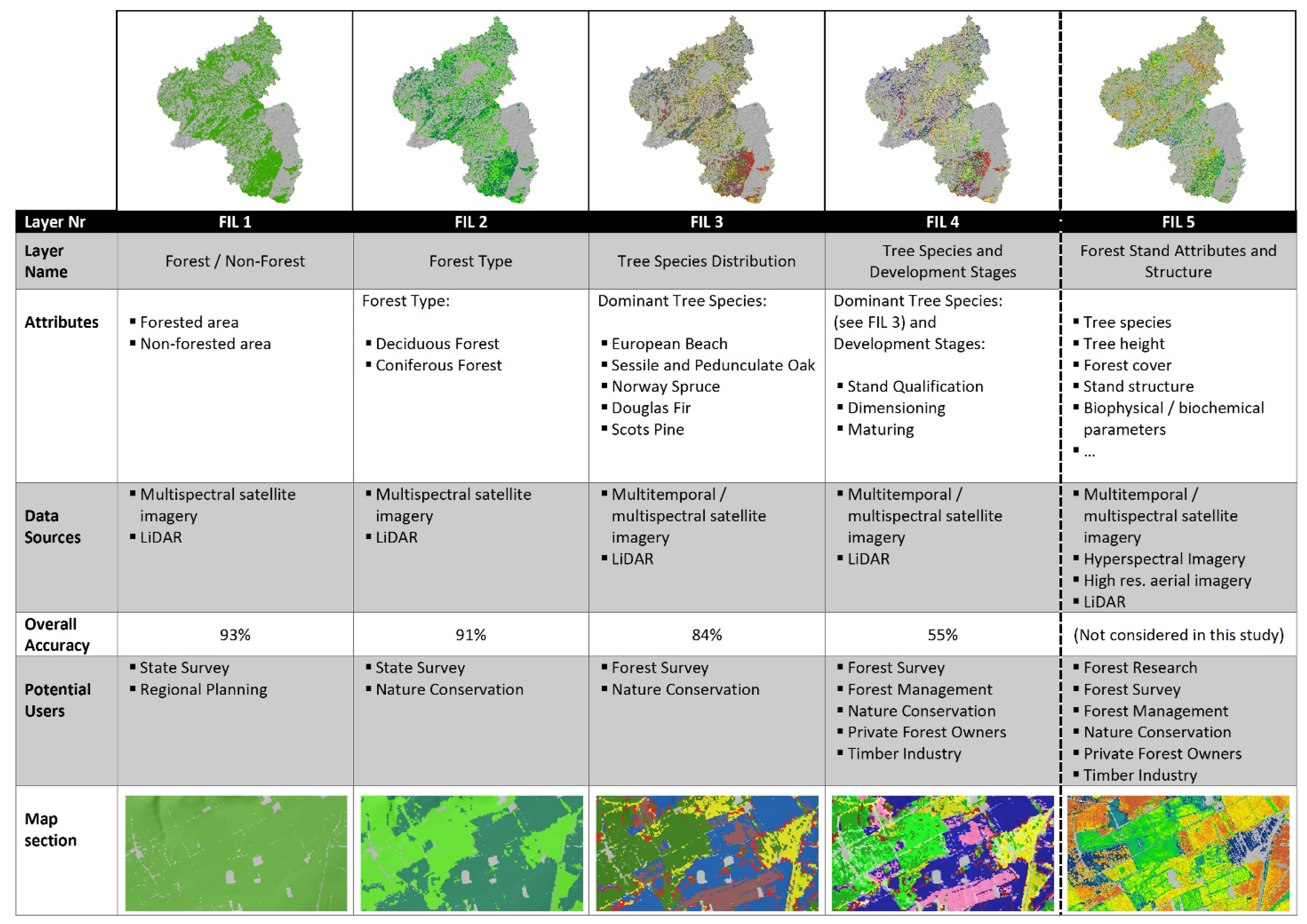
Update of existing forest/non-forest mapping products at a minimum mapping unit of 100 m² accommodating the needs of multiple authorities and users.

-

Forest type delineation at a minimum mapping unit of 100 m².

-

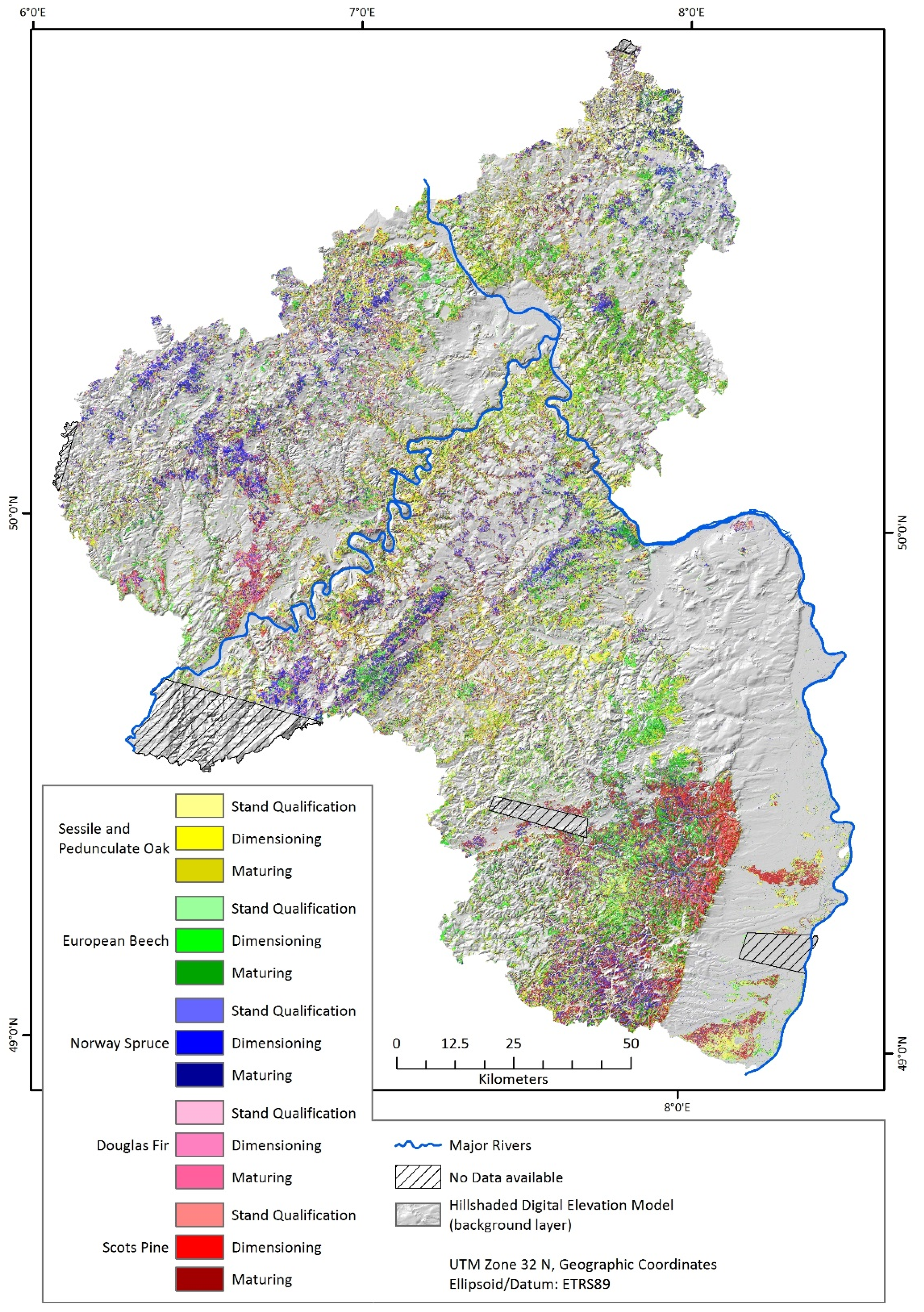
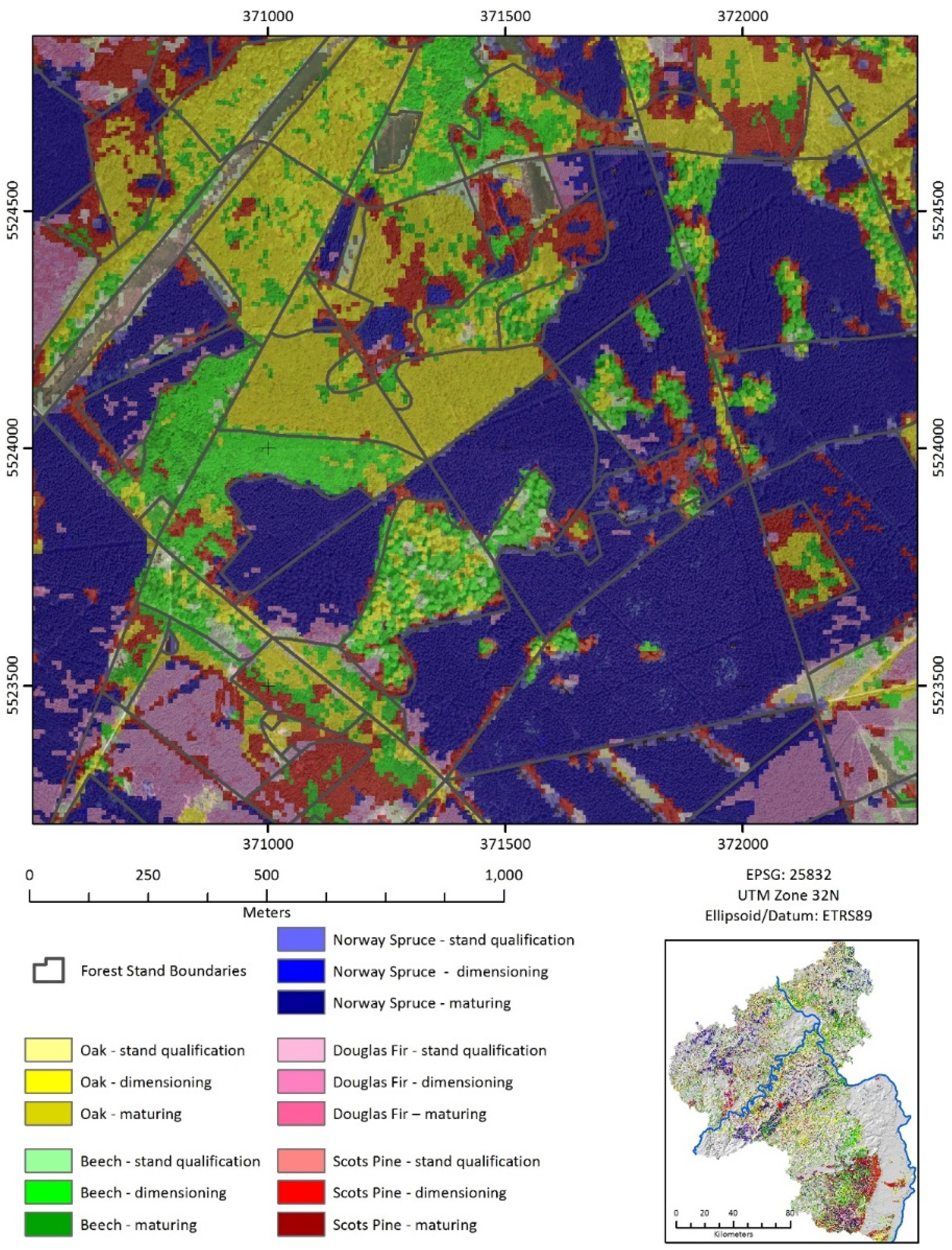
Spatial discrimination of five primary forest cover classes in RLP (Sessile and Pedunculate oak, European beech, Norway spruce, Douglas fir, and Scots pine) and three tree species development stages (stand qualification, dimensioning, and maturing).

-

Derivation of spatially explicit forest attributes at stand level (e.g., tree height, stand structure, total biomass, timber volume).

Particular attention should be paid to the following points:

-

Direct integration of existing forest inventory data as reference information.

-

Use of remote sensing-based mapping and inventory techniques compatible with standard field survey methods currently conducted in RLP.

-

Product consistency throughout the state of RLP.

-

High level of classification accuracy is required.

-

Approach must be based on satellite systems that provide reliable data availability.

-

Processing chain must be capable of being integrated into operative forest management.

1.3. Objectives

Based on the information need and the map product requirements specified by the state forest authorities, and taking into account challenging natural and forestal conditions (caused by climatic gradients and gradually changing site characteristics, as well as inherited management decisions and silvicultural practices applied in adjacent forests under different ownership or custody), the following objectives have been defined:

-

Design and application of an optimized data processing chain (geometric and radiometric corrections, data fusion techniques, classification algorithms) capable of handling data from multiple sources (multispectral satellite data from different sensor systems, official forest inventory data).

-

Integration of additional support data sets (airborne LiDAR, digital aerial orthophotos) for testing the validity of state forest inventory data used as reference information.

-

Production of satellite-based forest information layers for the complete federal state of RLP, comprising maps of forest/non-forest distribution, forest types (coniferous vs. deciduous), tree species at stand level, and tree species enhanced by three corresponding developmental stages.

-

Integration of the derived products in operational forest management tasks.

2. Study Area and Data

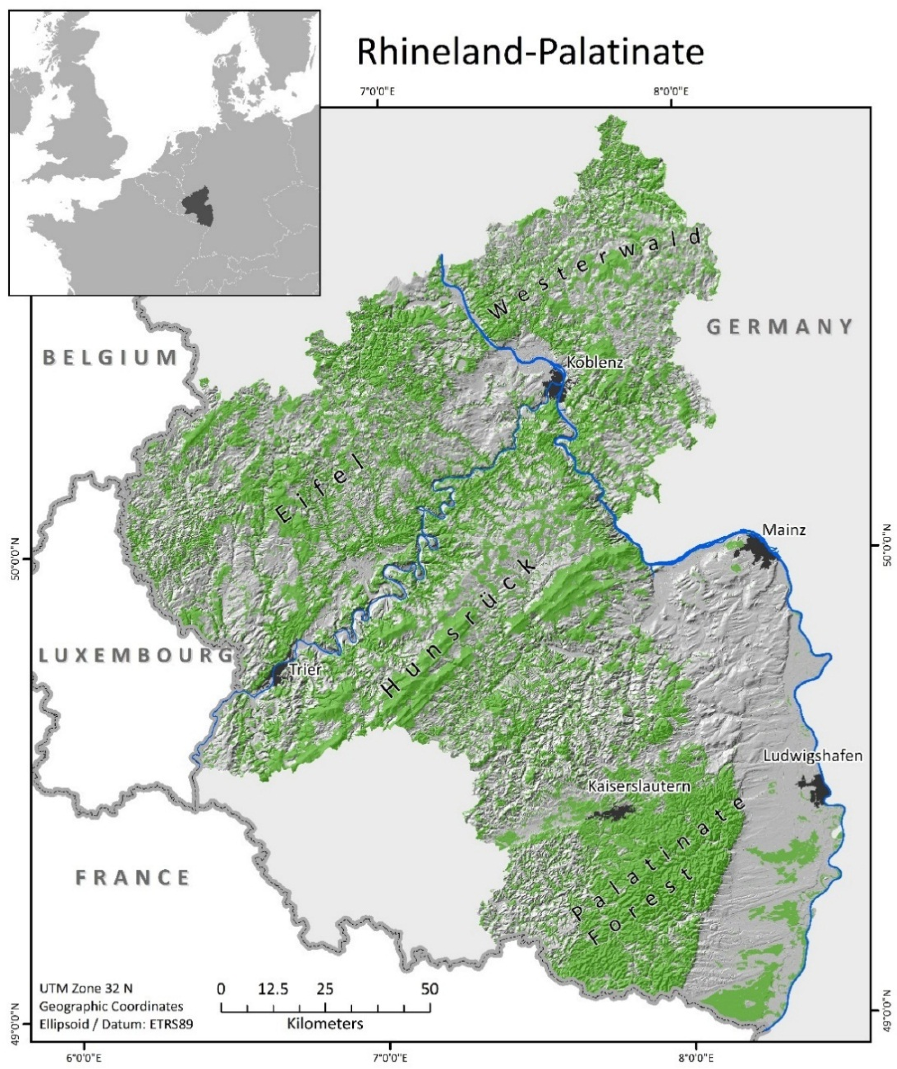
2.1. Study Area

The federal state of RLP is located in the west of Germany (see Figure 1). The state covers an area of about 19,850 square kilometers or 5.6% of the total geographical area of Germany. The landscape is dominated by the large Rhine River valley (crossing the state from southeast to northwest), the steep Moselle River valley, and the low mountain ranges of Eifel, Hunsrück, Westerwald (part of the Rhenish Hercynian uplands) and the Palatinate Forest low-mountain region. While the upper Rhine plain supports intensive agriculture, the low mountain ranges are characterized by steep, forested hills with elevations up to 800 m above sea level, and high plateaus dominated by farmland and pasture [23].

Figure 1. Study area: Detailed map of the study area highlighting the spatial distribution of forested areas (green).

Figure 1. Study area: Detailed map of the study area highlighting the spatial distribution of forested areas (green).

With a total forest cover of more than 8330 square kilometer or 42% of the state’s total area, RLP together with the state of Hesse, are Germany’s most densely wooded states. In RLP, the forest is predominantly in public ownership (approximately 75%). The most representative tree species are: 22% Norway spruce (Picea abies (L.) H. Karst.), 21% European beech (Fagus sylvatica L.), 20% Sessile oak (Quercus petraea (Mattuschka] Liebl.) and Pedunculate oak (Quercus robur L.), 11% Scots pine (Pinus sylvestris L.), and 6% Douglas fir (Pseudotsuga menziesii (Mirbel) Franco) [24].

The sub-Atlantic climate in the investigated area is modified by an altitude-related gradient. Mean annual rainfall ranges from 500 (upper Rhine plain) to 1300 mm (Hunsrück low-mountain range) and mean annual temperature from 6 to 11 °C [25]. According to the variability of climate and the natural environment, the study area is divided into 16 ecoregions with different forest growing conditions [23]. The growing season (defined as the period when daily mean temperatures exceed 10 °C on consecutive days) varies on average from 140 days in the mountainous parts to about 175 days in the river valleys. This leads to relatively large differences in phenology of forest species across the study area [23,25].

2.2. Data

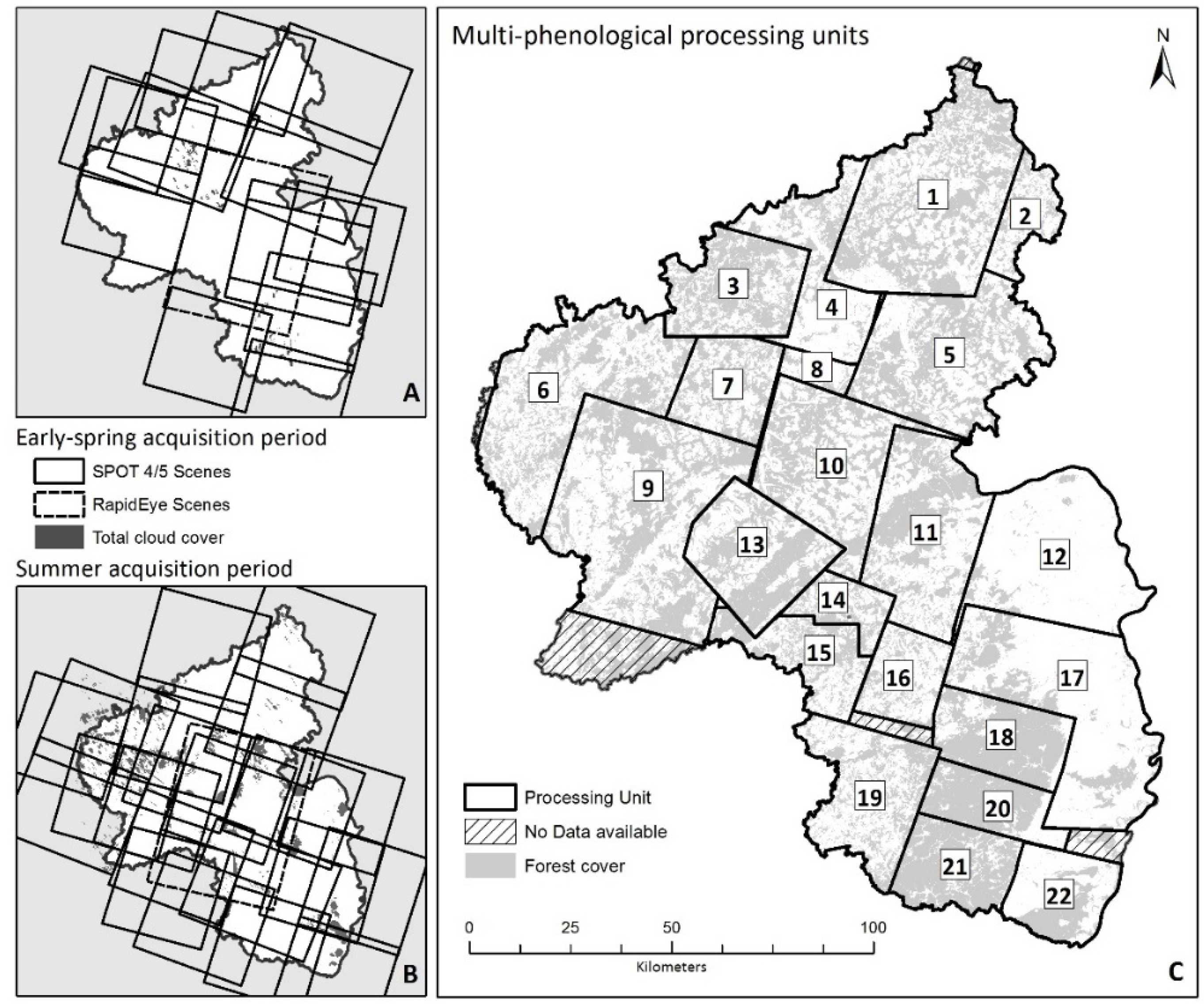
2.2.1. Satellite Data

Satellite data suitable for the derivation of detailed forest information layers at state level must meet the following requirements: sufficient spectral resolution to ensure reliable differentiation of forest types and tree species [26]; high spatial resolution to accurately depict small forest stands and adequately characterize forest biophysical parameters [27]. Additionally, the system should provide frequent repetition cycles, because phenology information inherent in multi-temporal observation is a key asset for separating otherwise spectrally similar species [28,29,30]. In the pilot study [18] it became apparent that in order to differentiate between deciduous tree species, satellite images from at least two phenological stages are necessary: foliage formation and fully developed foliage. The start of the phenological phase of foliage formation is sensitive to regional climate conditions with substantial variation within and among species [31,32]. In the mountainous regions of South and Southwest Germany, foliage formation of European Beech starts significantly earlier (on average 7 days) than Sessile Oak [23,33,34]. Most importantly, the leaf development phase (bud burst followed by the development of small leaves with folded blades and subsequent development of small unfolded leaves) with significant differences between both species groups [35]) lasts two to three weeks and thereby creates a substantial time window for the acquisition of satellite imagery with high discrimination capacities. At present, several satellite systems are able to fulfill the requirements listed above almost perfectly (e.g., SPOT-4/5/6/7, RapidEye, and the forthcoming Sentinel-2).

To map RLP forest, we initially used 28 SPOT-5 and 4 SPOT-4 scenes, attempting to cover the two most important phenological stages for forest species discrimination. The multispectral images were acquired with three bands: visible green (500–590 nm), visible red (610–680 nm), and near-infrared (780–890 nm) at 10-m spatial resolution, combined with shortwave-infrared band (1580–1750 nm) acquired at 20-m spatial resolution [36]. Due to cloud cover and competition among customer orders, the extension of both acquisition periods and the inclusion of two additional RapidEye scenes, covering the central part of the state during the phenological stage of foliage formation, became necessary. The RapidEye sensor is equipped with a multispectral push broom imager with spatial resolution of 6.5 m that captures data in five spectral bands: visible blue 440–510 nm), visible green (520–590 nm), visible red (630–685 nm), red edge (690–730 nm), and near-infrared (760–850 nm) [37]. Details of the scenes used are shown in Table 1; spatial extent, overlap and cloud cover are mapped in Figure 2 for both acquisition periods.

Table 1. Available satellite data and resulting processing unit characteristics.

Processing Unit		Early-Spring Acquisition Period			Summer Acquisition Period			Details
ID	Area (km2)	Acquisition date	Sensor	Incidence angle	Acquisition date	Sensor	Incidence angle	Total cloud cover (%)	Forested area (%)
1	1673	24/04/2011	SPOT4	8.3	31/07/2008	SPOT5	19.8	1.9	44
2	315	25/04/2011	SPOT5	29.7	31/07/2008	SPOT5	19.8	0.7	31
3	752	05/05/2008	SPOT5	20.6	16/08/2009	SPOT5	19.6	1	54
4	755	10/05/2008	SPOT5	14.2	16/08/2009	SPOT5	19.6	0.1	23
5	1294	25/04/2011	SPOT5	29.7	31/07/2008	SPOT5	19.7	1	40
6	1510	05/05/2008	SPOT5	20.6	15/07/2008	SPOT5	22.5	12.3	35
7	553	05/05/2008	SPOT5	20.6	16/08/2009	SPOT5	19.6	12.9	36
8	137	22/05/2010	SPOT5	25.1	16/08/2009	SPOT5	19.6	0	18
9	1977	05/05/2008	SPOT5	20.6	31/08/2009	SPOT5	4.7	1	41
10	1108	06/04/2010	RapidEye	3.8	03/07/2006	SPOT5	13.9	0	42
11	1132	18/04/2010	SPOT5	27.7	03/07/2010	SPOT5	21.2	6.3	51
12	1288	25/05/2009	SPOT5	17.1	05/08/2009	SPOT5	3.4	0.8	5
13	833	06/04/2010	RapidEye	3.8	07/08/2010	RapidEye	7.6	0	53
14	287	06/04/2010	RapidEye	3.8	08/07/2010	SPOT5	22.4	0	46
15	532	06/04/2010	RapidEye	3.8	08/07/2010	SPOT5	22.4	0	43
16	423	06/04/2010	RapidEye	3.8	07/08/2010	RapidEye	7.6	32.2	37
17	1593	20/04/2009	SPOT4	17.2	31/08/2005	SPOT5	1.3	0.2	20
18	611	20/04/2009	SPOT4	17.2	31/08/2005	SPOT5	1.3	0.9	74
19	869	10/05/2008	SPOT5	10.8	31/07/2008	SPOT5	19.8	1	36
20	459	20/04/2009	SPOT4	17.2	05/09/2005	SPOT5	2.6	3	74
21	575	07/04/2010	SPOT5	12.3	05/09/2005	SPOT5	2.6	1.3	80
22	519	07/04/2010	SPOT5	12.3	14/07/2010	SPOT5	10.8	6.4	32

Table 1. Available satellite data and resulting processing unit characteristics.

Processing Unit		Early-Spring Acquisition Period			Summer Acquisition Period			Details
ID	Area (km2)	Acquisition date	Sensor	Incidence angle	Acquisition date	Sensor	Incidence angle	Total cloud cover (%)	Forested area (%)
1	1673	24/04/2011	SPOT4	8.3	31/07/2008	SPOT5	19.8	1.9	44
2	315	25/04/2011	SPOT5	29.7	31/07/2008	SPOT5	19.8	0.7	31
3	752	05/05/2008	SPOT5	20.6	16/08/2009	SPOT5	19.6	1	54
4	755	10/05/2008	SPOT5	14.2	16/08/2009	SPOT5	19.6	0.1	23
5	1294	25/04/2011	SPOT5	29.7	31/07/2008	SPOT5	19.7	1	40
6	1510	05/05/2008	SPOT5	20.6	15/07/2008	SPOT5	22.5	12.3	35
7	553	05/05/2008	SPOT5	20.6	16/08/2009	SPOT5	19.6	12.9	36
8	137	22/05/2010	SPOT5	25.1	16/08/2009	SPOT5	19.6	0	18
9	1977	05/05/2008	SPOT5	20.6	31/08/2009	SPOT5	4.7	1	41
10	1108	06/04/2010	RapidEye	3.8	03/07/2006	SPOT5	13.9	0	42
11	1132	18/04/2010	SPOT5	27.7	03/07/2010	SPOT5	21.2	6.3	51
12	1288	25/05/2009	SPOT5	17.1	05/08/2009	SPOT5	3.4	0.8	5
13	833	06/04/2010	RapidEye	3.8	07/08/2010	RapidEye	7.6	0	53
14	287	06/04/2010	RapidEye	3.8	08/07/2010	SPOT5	22.4	0	46
15	532	06/04/2010	RapidEye	3.8	08/07/2010	SPOT5	22.4	0	43
16	423	06/04/2010	RapidEye	3.8	07/08/2010	RapidEye	7.6	32.2	37
17	1593	20/04/2009	SPOT4	17.2	31/08/2005	SPOT5	1.3	0.2	20
18	611	20/04/2009	SPOT4	17.2	31/08/2005	SPOT5	1.3	0.9	74
19	869	10/05/2008	SPOT5	10.8	31/07/2008	SPOT5	19.8	1	36
20	459	20/04/2009	SPOT4	17.2	05/09/2005	SPOT5	2.6	3	74
21	575	07/04/2010	SPOT5	12.3	05/09/2005	SPOT5	2.6	1.3	80
22	519	07/04/2010	SPOT5	12.3	14/07/2010	SPOT5	10.8	6.4	32

Due to the extended acquisition periods in combination with cloud coverage and the varying observation angles of the SPOT satellites, it was impossible to classify the whole study area in one process, as intended. Instead, the considered satellite data, representing the phenological stage of foliage development and full foliage, created a mosaic of intersecting footprints that resulted in 22 individual bi-temporal data stacks (see Figure 2c). The stacks were compiled individually according to the phenological situation in the processing units. Thus, the annual variation in phenology during the observation period, especially that of early foliage development, resulted in limited comparability of the extracted reference signatures across the 22 data stacks, ranging in size from just over 140 km² ha to more than 1900 km² (average size 875 km²). Consequently, separate processing of the data stacks as individual processing units was necessary.

Figure 2. (a) Available satellite data for the early-spring acquisition period, representing the phenological stage of foliage development; (b) Available satellite data for the summer acquisition period, representing the phenological stage of full foliage; (c) Resulting processing units.

Figure 2. (a) Available satellite data for the early-spring acquisition period, representing the phenological stage of foliage development; (b) Available satellite data for the summer acquisition period, representing the phenological stage of full foliage; (c) Resulting processing units.

2.2.2. Forest Inventory Data

The state forest authorities provided detailed forest inventory data for all state and communal forests, through a digital forest-information-system. This information system documents approximately 75% of the state’s forests. The inventory data are collected as part of the regular forest surveys carried out at 5- to 10-year intervals, complemented by expert assessment at stand level [20]. The exact geolocation and extent are stored in a GIS database, associated with numerous silvicultural attributes (such as species composition, stand structure, tree development stages, stand density, and forest volume) and additional site characteristics (such as growing conditions, geology, soil, climate, and stand history). For each tree species within a forest stand, age class, stand structure and silvicultural measures (such as thinning operations and selective cuttings) are described by a multifunctional definition, which is based on the following distinct development stages: establishment (stand foundation and establishment of seedlings), qualification (thickets), dimensioning (crop tree definition and selective thinning), and maturation (timber stage). A forest stand may include up to 16 different tree species; on average, it comprises two or three main tree species in mixtures. In this study, we focus on five main stand-forming tree species that collectively represent more than 80% of the total forest in RLP [38]. Stand polygons range in size from 0.05 to 80 ha (average 3.5 ha). In total, more than 185,000 individual stand descriptions are stored in the forest inventory database. The database provided by the state forest administration is primarily designed for forest management purposes. Accordingly, the within-stand distribution of tree species and development stages are only qualitatively expressed in the form of estimated area proportions but are not explicitly localized within the stand, which is seen as a major limitation of the data [20,39].

2.2.3. Supplementary Data

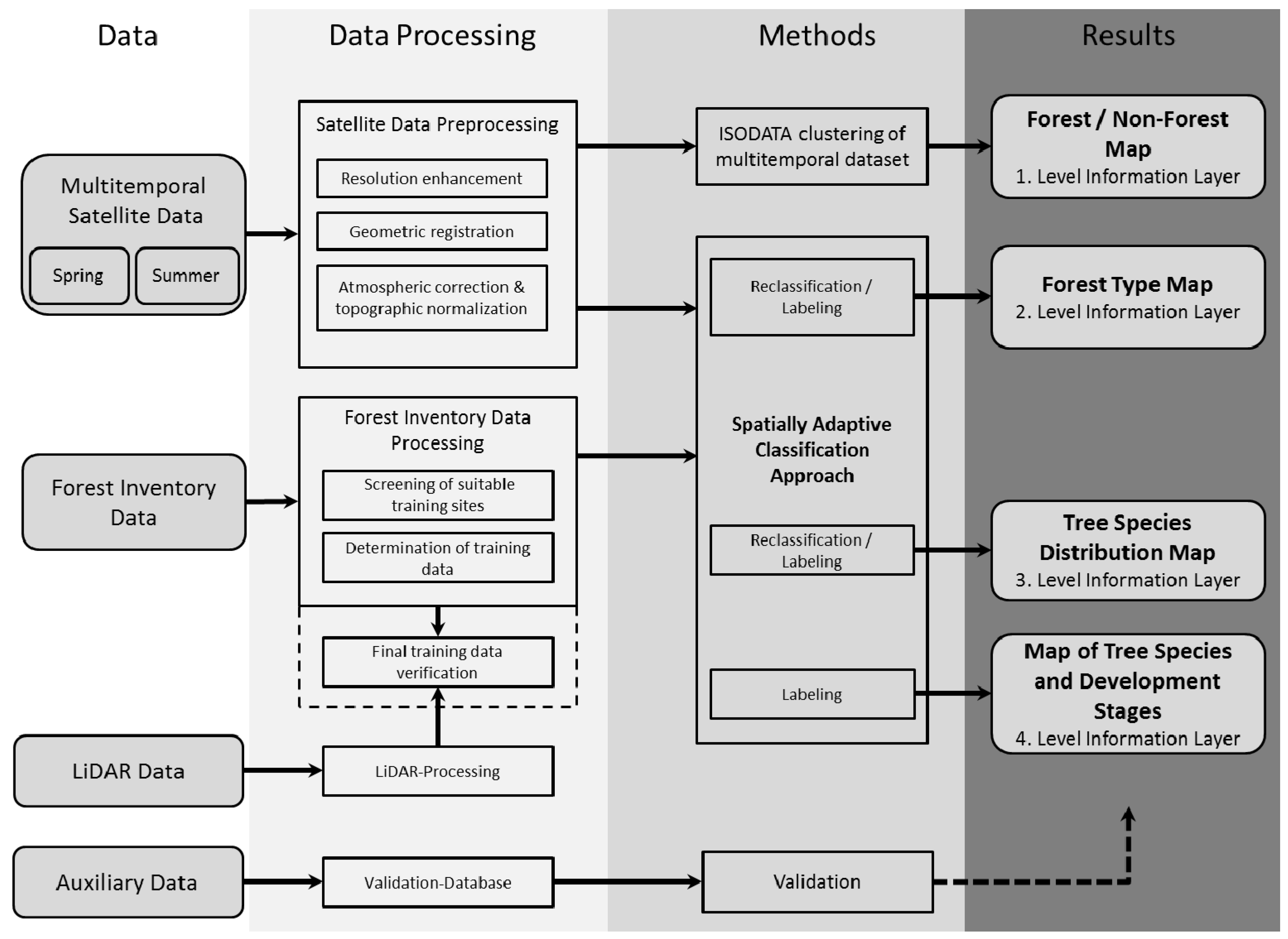
Airborne LiDAR data are available for the entire federal state. The data were acquired by the state’s survey authorities during a ten-year period. The state survey agency provides first-return points and filtered ground points with an average point density of 4 m⁻². A 1-m resolution digital surface model (DSM) and a digital ground model (DGM) were calculated from the point data. A canopy height model (CHM) was created by subtracting the digital surface model from the digital surface model [40]. The acquisition of LiDAR data over the complete federal state was conducted over a period of 10 consecutive years, with the consequence of substantial differences in data quality (e.g., point densities) between the individual data segments. This did not allow to use LiDAR-data as a consistent information layer in the pixel-based classification. However, the LiDAR-derived canopy height information proved to be extremely useful to quality-check and adjust inventory database entries on stand development phases. Additionally, current high-spatial-resolution aerial imagery, topographic and thematic maps, as well as the official topographical cartographic information system are available for the study area.

3. Data Preparation

Considering the requirements defined by the state forest service, the approach must be capable of being integrated into operative forest management. Therefore, entire processing chain is designed to optimize the available data (satellite and reference) to achieve the required level of accuracy, and to integrate the preparation and classification methods into a single processing chain (see Figure 3).

Figure 3. Schematic of the spatially adaptive classification approach to deriving high-resolution forest information layers.

Figure 3. Schematic of the spatially adaptive classification approach to deriving high-resolution forest information layers.

3.1. Preprocessing of Satellite Data

With regard to the subsequent mapping and classification processes, the following steps were applied to optimize the quality of the SPOT-4/5 and RapidEye data.

3.1.1. Resolution Enhancement

Multispectral satellite data with medium spatial resolution have only been of limited use for the identification of species compositions, especially in forests with high tree species diversity [41,42]. Therefore, the reduced spatial resolution of the SPOT-4/5 infrared band was adjusted to match the 10-m pixel size of the visible and near-infrared bands (1–3). The resolution enhancement was performed using a local correlation approach that preserves the spectral characteristics of the low-resolution input band and transfers the textural properties of the high-resolution reference to the SPOT-infrared channel [43]. This approach was found to be appropriate in an independent comparison study [44]. The resulting enhanced spatial resolution is expected to improve the identification of small forest structures. For RapidEye data, no further resolution enhancement was necessary.

3.1.2. Geometric Registration

Multi-temporal image analysis requires accurate georeferencing and correction of distortions. The georegistration of SPOT-4/5 and RapidEye data utilizes a digital elevation model to compensate relief-dependent pixel displacements. Especially in the mountainous regions of the study area, relief-dependent distortions could degrade the classification results [45,46]. To ensure sub-pixel accuracy, an automated search algorithm was used to identify large sets of ground control points [47]. The resulting ortho-projected images were transformed to the local coordinate system (Gauss-Krüger Zone 2). Sub-pixel accuracy was achieved, fulfilling all requirements for multi-temporal image analysis and guaranteeing efficient integration of the external geo-databases.

3.1.3. Atmospheric Correction

A major problem for mapping forest types in mountainous regions is radiometric distortion of the measured signal due to topography-dependent illumination effects [48,49,50]. The magnitude of these effects varies as a function of solar inclination and azimuth as well as slope incline and aspect [51,52]. In the mountainous regions of our study area, these effects are particularly pronounced at Eifel, Hunsrück, and Westerwald, where major morphological features extend almost orthogonally to the illumination azimuth (see Figure 1). Since simple topographic normalization strategies such as Lambert cosine correction can lead to overcorrection effects, the concurrent correction of topographic and atmospheric influences, explicitly accounting for direct and diffuse irradiance fluxes, is considered one of the most efficient strategies for compensating terrain-dependent radiometric distortions [53,54,55]. The applied radiometric correction scheme comprises sensor calibration using adjusted calibration functions and full radiative transfer modeling. The integrated radiometric correction was performed using AtCPro (Atmospheric Correction and Processing of Multi- and Hyperspectral Data) software, which is based on the 5S model by Tanré et al. [56]. AtCPro considers direct and diffuse radiance terms, which are modified according to local elevation, slope and aspect derived from the digital elevation model [55]. Several studies confirm that the concurrent correction of topographic and atmospheric influences leads to substantial improvements in classification results [51,57,58,59].

3.2. Forest Inventory Data Processing

The forest inventory data provided by the state forest administration is primarily designed for forest management purposes. With the requirement to develop an approach with operational capacity for repeated state forest inventories, it was essential to establish an optimized processing scheme to guarantee the direct integration of available forest inventory data into the classification process. The following measures were taken to achieve this objective.

3.2.1. Screening of Suitable Training Sites

Pure stands occur only occasionally in near-natural forests; consequently, all available forest inventory data had to be screened for potential training sites. The tree species variability within the different stands precludes immediate integration of forest inventory information for generating representative training data for the classification process (stand distribution of tree species and tree development stages are only qualitatively expressed in the database in the form of estimated area proportions, but are not explicitly georeferenced within a stand). Consequently, spatial discrimination of suitable training areas representing specific tree species and development stages was necessary.

From the available forest inventory data, GIS-based selection was performed, grouping forest stands into 15 thematic classes according to main tree species and development stages. To be selected, a specific class had to be the dominant species in terms of areal coverage within the stand. For each selected stand, image subsets of the principal-component-transformed satellite data set were extracted by intersecting the image with the corresponding stand geometries. Each of the image subsets was spatially segmented into five spectral subclasses by applying an ISODATA clustering algorithm. Following an approach similar to the method of guided clustering presented by Bauer et al. [60] and Reese et al. [61], it is possible to identify the largest spectrally homogeneous areas within each stand. Based on transformed divergence values, high-spatial-resolution aerial imagery, forest inventory descriptions, and field measurements, the derived clusters were labeled either as representative of one of the fifteen thematic classes or as ambiguous. Thereby, all areas composed of mixed canopies, those at stand boundaries, or affected by other disturbances were described as ambiguous. All accepted clusters were marked as potential training areas and stored in a GIS database. The guided clustering excluded approximately 40% of the GIS-selected polygons for the tree species classes Norway spruce and Douglas fir, and up to 60% for Sessile and Pedunculate oak, European beech, and Scots pine. For further use, only the most homogeneous and spectrally representative areas within a forest stand were retained in the final GIS-database.

3.2.2. Determination of Training Data

For the final extraction of spectral references, a 100 m × 100 m regular sampling grid was superimposed on the identified potential training areas. By using a regular point grid, spatial autocorrelation among neighboring reference pixels was avoided [62,63]. Spectral reference information to represent the 15 thematic classes was extracted from more than 540,000 reference points and stored in a GIS-database. This resulted in a consistent set of reference data for each of the thematic classes. The class descriptors were characterized by approximate normal distributions.

3.2.3. Verification of Training Data

To verify that the derived training data represent not only the correct tree species but also the appropriate development stage, a final data quality check was performed. Due to lack of timeliness of part of the forest inventory data, as well as short-term events (silvicultural treatment, storm fall, or insect calamities) it was felt necessary to verify whether the database entries on development stages were consistent. Comparison with stand-wise statistics of crown height distribution derived by the airborne laser scanning ensured that all training data were within the expected tree height distribution for a specific development stage.

4. Methods

This section presents the methods used to derive state-wide forest information layers for RLP, comprising an up-to-date forest/non-forest map and high-spatial-resolution forest type maps and tree species distribution maps. Additionally, it presents a validation concept to ensure the required levels of accuracy, and to explore the implications for further developments and adaptations.

4.1. Derivation of High-Resolution Forest Information Layers

4.1.1. Forest/Non-Forest Stratification

To derive a first forest information layer and focus the subsequent processing steps only on relevant areas, the satellite imagery was merged into a multi-phenological data-stack, and then stratified into forest and non-forest areas via unsupervised classification using the ISODATA algorithm [64]. The resulting spectral classes there assigned to the informational classes forest and non-forest by means of high resolution aerial imagery.

4.1.2. Forest Type Map

To fulfill the increasing need for information on the multiple roles of forests, large-area forest type mapping projects should become a key component in providing accurate and up-to-date information on the spatial distribution and species composition of forest ecosystems. Several projects have mapped transnational or even pan-European forest resources [15,65,66,67]. In order to evaluate the potential advantages of adaptive classification methods in combination with high-spatial-resolution data and complex satellite data preprocessing to increase the map accuracy of large-area forest type maps, a tree type map was derived from our spatially adaptive classification product (see Section 4.1.3). For this purpose the thematic classes Sessile and Pedunculate oak, European beech, Norway spruce, Douglas fir, and Scots pine (in the tree species development stages stand qualification, dimensioning, and maturing) were reclassified into the forest type classes deciduous forest and coniferous forest.

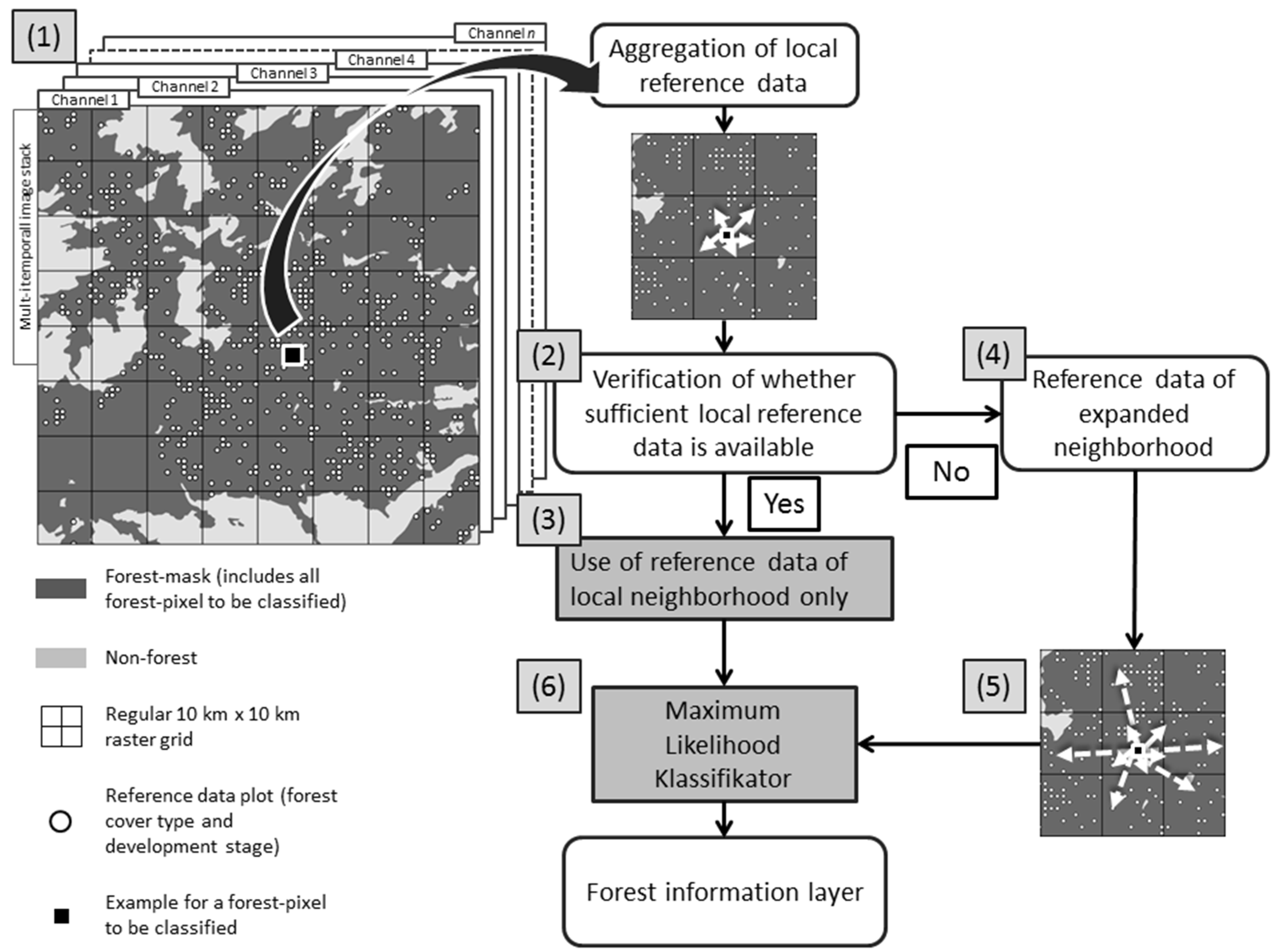
4.1.3. Map of Tree Species Distribution and Tree Species Development Stages

The temporal and spatial consistency of reflectance properties is of particular importance when addressing large study areas characterized by different ecoregions [68]. In RLP, spatially variable growth conditions (depending on regional climate, soil, silvicultural practice) cause the same forest cover class to exhibit different spectral responses at the time of observation, particularly during early phenological development stages. During later phenological stages, this spectral variability becomes less relevant because canopy development is largely completed. However, the necessity to consider multi-phenological satellite data in order to achieve the required level of classification accuracy, and additional regional differences caused by local variances in silvicultural practice (especially between public and private forests) impose the need for regionally adapted procedures. In order to overcome these limitations on classifier performance, a spatially adaptive classification approach was introduced [18].

Rather than attempting to derive homogenous strata from the satellite imagery, the spatially adaptive classification generates an efficient organizational structure and ensures flexible access to the available reference data. This procedure avoids additional preliminary processing steps and ensures access to the whole training dataset. For this study, the organizational design was based on a regular 10 km × 10 km grid, superimposed onto RLP. Thereby, each of the 10 km × 10 km quadrants represents a separate spatial reference unit, within which the available training data are used to parameterize the classifier. Considering the preconditions (training data descriptors were characterized by approximate normal distributions), the maximum likelihood classifier appears an appropriate choice. Spatially adaptive parameterization accounts for existing environmental, phenological, and management gradients across the spatial units. The actual size of the sampling quadrants was selected to allow a sufficient amount of training data in each quadrant for most of the thematic classes. According to Swain and Davis [69], the per class number of training samples in a maximum likelihood classification should not be less than ten times the number of dimensions in the feature space (i.e., 10 × 4 bands = a minimum of 40 samples).

Spatially adaptive classification involves the following steps (see Figure 4):

(1)

Identification of the local reference unit within the unknown forest-pixel to be classified;

(2)

Verification of whether sufficient reference data per thematic class are available within this unit;

(3)

If so, these data are used directly to parameterize the maximum likelihood classifier;

(4)

Otherwise (reference data are insufficient for one or more thematic classes within the starting reference unit), the considered search area for the respective thematic class is expanded by considering neighboring reference units;

(5)

In case a thematic class is still not represented by sufficient data, the training procedure falls back on a basic reference set derived from the entire reference database;

(6)

Derivation of final maps uses a maximum likelihood classification based on locally optimized training data.

Figure 4. Flowchart of the spatially adaptive classification approach.

Figure 4. Flowchart of the spatially adaptive classification approach.

For further details on the design and implementation of the spatially adaptive classification approach, see Stoffels et al. [18].

4.2. Validation

Traditional statistical methods use an independent validation dataset to assess the accuracy of derived forest cover maps. Presented with the challenges of operational sustainable forest management, statistical accuracy assessment can only assess the quality of the approach, not its suitability for inclusion in forest inventory schemes.

To assess the accuracy of the resulting forest information layers, different sets of validation points were selected. Independent data from the official topographical cartographic information system and the federal forest survey were used to assess the accuracy of the forest/non-forest stratification and forest type mapping. A probability sampling design was chosen to validate the accuracy of the tree species distribution map and the tree species development stages. The validation points were derived using delineation of well-defined stands from the forest inventory GIS database. Within the selected stands, more than 1500 points of interest were randomly selected, considering the requirements of proportional adjustment. Every point of interest was characterized by forest inventory data and verified by visual inspection of very high spatial resolution aerial imagery. Points that could not be unambiguously assigned to one stand (e.g., points in mixed stand, points at stand boundaries) were excluded from the sample.

The forest information layers were analyzed by means of confusion matrices [70,71] that were used to calculate producer’s accuracy, user’s accuracy, overall accuracy [72,73], and Cohen’s kappa coefficient [74,75].

To account for the challenges of operational sustainable forest management and to assess the potential for integrating the derived maps into current forest inventory schemes, a validation workshop was held with forest assessors. These forest survey experts reviewed the resulting data and maps with a special focus on the stand-specific accuracy of tree species distribution maps, the scale of the resulting maps, applicability to field surveys, limitations on practical application of the product, and further developments.

5. Results and Discussion

5.1. Forest/Non-Forest Stratification

The derived first FIL, representing state-wide forest/non-forest stratification, was validated using 6274 points from the official RLP topographical cartographic information system, achieving an overall classification accuracy of more than 93%. The forest/non-forest map represents a forest information layer that is capable of updating the topographical cartographic information system (e.g., including newly-afforested areas or excluding new development areas).

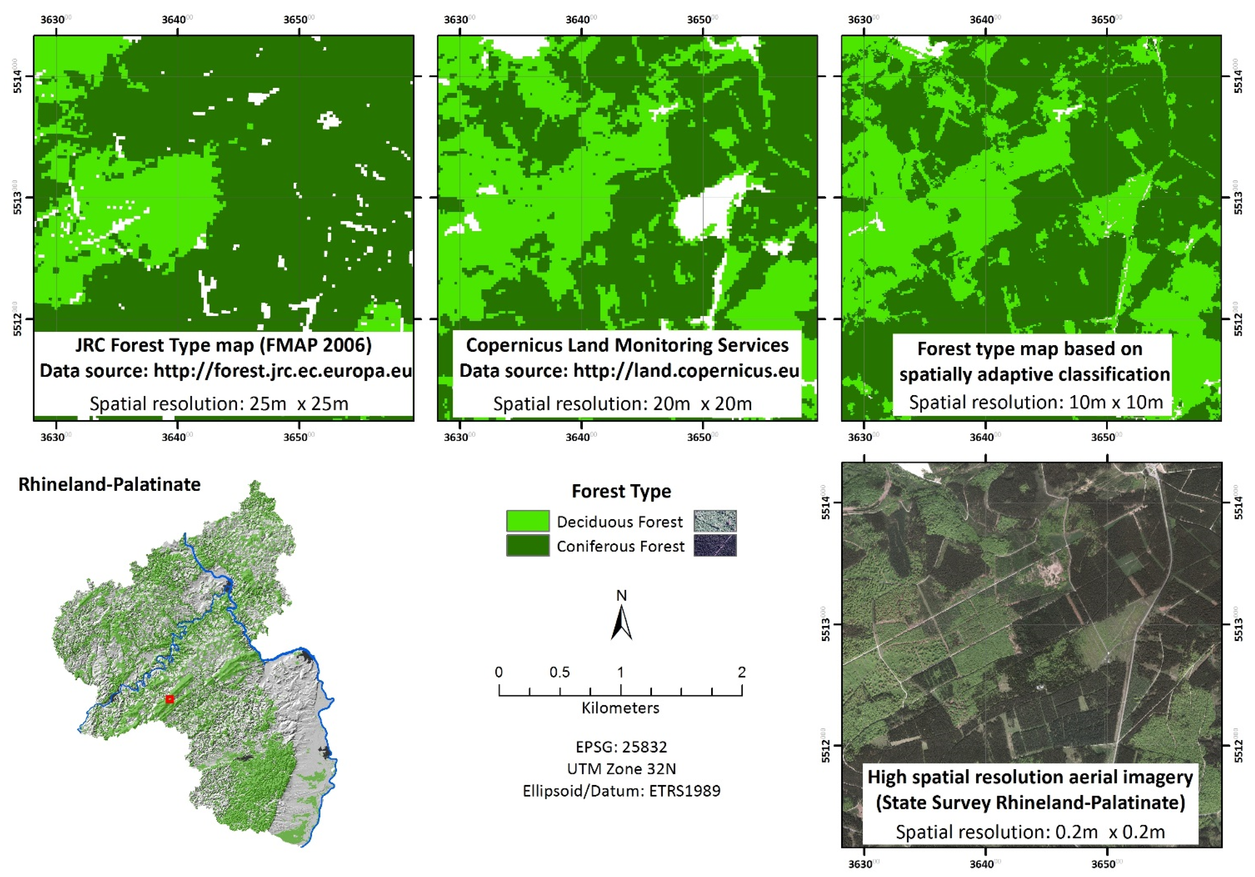
5.2. Forest Type Stratification

A forest type map (FIL 2) was derived from our spatially adaptive classification product to evaluate the potential for more accurate large-area forest type mapping via adaptive classification methods combined with high spatial resolution data and complex satellite data preprocessing. For direct comparison, two freely available pan-European forest type products were selected: the European Commission’s Joint Research Center (JRC) Forest Type Map 2006 [15] and the European Environment Agency’s GIO (GMES/Copernicus initial operations land) land High-resolution Layers (HRL) Forest Type product [76]. JRC provides its forest type map (FTYP 2006) at 25 m spatial resolution (the proposed INSPIRE grid standard) containing broadleaved and coniferous categories. Inputs consisted of high-spatial -resolution SPOT4/5 and IRS-LISS-3 satellite imagery (acquired in 2005 and 2006) and multi-temporal MODIS data. The map product is freely available from the JRC website (http://forest.jrc.ec.europa.eu/download/data/forest-data-download/). The European Environment Agency’s high-resolution forest type map is available at 20 m spatial resolution. The forest type layer was mapped on the basis of high spatial resolution IRS-P6/RESOURCESAT and RapidEye imagery, acquired in 2011 and 2012. Additionally, medium-resolution IRS-A WiFS data were used. The forest type product maps coniferous and broadleaved trees at a minimum mapping unit of 0.5 ha [77]. The product is available as a web mapping service from the Copernicus Land Monitoring Services website (http://land.copernicus.eu/pan-european/high-resolution-layers/forests).

Validation of Forest Type Information Layers

Based on the forest type mapping results, Table 2 shows the percentages of tree species for the whole study area compared with those estimated during a state-wide forest survey in 2008 [24] and JRCs 2006 forest-type mapping product [15].

Table 2. Proportional coverage of forest types for Rhineland-Palatinate from official forest survey estimation [78] compared with the JRC forest-type map, Copernicus HRL, and the proposed spatially adaptive classification.

Forest Type	Forest Survey RLP	JRCs Forest-Type Map 2006	Copernicus High-Resolution Layers	Spatially Adaptive Classification
Deciduous Forest	60%	59.6%	67.9%	53.8%
Coniferous Forest	40%	40.4%	32.1%	46.2%

Table 2. Proportional coverage of forest types for Rhineland-Palatinate from official forest survey estimation [78] compared with the JRC forest-type map, Copernicus HRL, and the proposed spatially adaptive classification.

Forest Type	Forest Survey RLP	JRCs Forest-Type Map 2006	Copernicus High-Resolution Layers	Spatially Adaptive Classification
Deciduous Forest	60%	59.6%	67.9%	53.8%
Coniferous Forest	40%	40.4%	32.1%	46.2%

The proportional coverage of JRCs forest type map from 2006 almost perfectly matches the official survey estimation of 2012. The derived percentages of both Copernicus HRL and our classification deviate from the state forests survey values by 7.9% and 6.2%, respectively. However, the comparison does not take into account the spatial distribution and fragmentation of the forested area. The state-wide terrestrial forest inventory (2012–2013) was used to assess the accuracy of the predicted forest types. The state forest inventory was conducted as a supplement to the national forest inventory (Bundeswaldinventur 3), based on a 2 km × 2 km cluster sampling grid. Each cluster is represented by a square of 150 m side length with sampling plots in the four corners, on which angle-count sampling and several plot measurements were conducted [79]. To assess the accuracy of forest type, only data on tree species distribution were used. If a sampling plot was characterized by more than 80% deciduous trees it was labeled “deciduous”; if it was covered by more than 80% coniferous trees it was labeled “coniferous.” All other ambiguous sampling points were excluded from the accuracy assessment. From the resulting 4480 validation points, only those covered by the forest type maps were considered for further analysis. Because of cloud cover, areas not covered by the resulting maps, and differences in spatial resolution, the number of validation points used was 3940 for the spatially adaptive classification product, 4149 for JRCs forest-type mapping product, and 3995 for the Copernicus high-resolution layers.

The forest type map derived from our spatially adaptive classification achieved a substantially higher overall accuracy of 90.72%, compared to 81.18% for the JRC product and 78.48% for Copernicus (see Table 3 for further detail). User and producer accuracies for both forest types differed considerably depending on which map product was examined. Overall, user and producer accuracies are higher for the spatially adaptive classification (Deciduous forest: 90.93% and 89.79% for user’s and producer’s accuracy, compared to 85.80% and 72.25% for JRC, and 92.34% and 74.55% for Copernicus, respectively. Coniferous forest: 90.51% and 91.58% for user’s and producer’s accuracy, compared to 72.33% and 85.84% for JRC, and 70.86% and 90.91% for Copernicus, respectively).

Table 3. Summary of forest-type validation (based on 4480 validation points).

	JRCs Forest-Type Mapping Product		Copernicus High-Resolution Layers		Spatially Adaptive Classification
	Error of		Error of		Error of
	Omission	Commission	Omission	Commission	Omission	Commission
Deciduous Forest	27.75	14.20	25.45	7.66	10.21	9.07
Coniferous Forest	14.16	27.67	9.09	29.14	8.42	9.49
Overall Accuracy	78.48%		81.18%		90.71%
Area covered	100%		91%		96%

Table 3. Summary of forest-type validation (based on 4480 validation points).

	JRCs Forest-Type Mapping Product		Copernicus High-Resolution Layers		Spatially Adaptive Classification
	Error of		Error of		Error of
	Omission	Commission	Omission	Commission	Omission	Commission
Deciduous Forest	27.75	14.20	25.45	7.66	10.21	9.07
Coniferous Forest	14.16	27.67	9.09	29.14	8.42	9.49
Overall Accuracy	78.48%		81.18%		90.71%
Area covered	100%		91%		96%

Figure 5 shows map views of all three forest type maps in comparison with high spatial resolution aerial imagery of a densely forested area in the Hunsrück low-mountain range. The area is covered with mature deciduous and coniferous trees and has not changed in composition or structure since 2006. High map accuracy and the spatial resolution of 10 m × 10 m leads to good spatial consistency with the forest type map derived from of our spatially adaptive classification. In this case, the 25 m × 25 m spatial resolution of the JRC map is not suitable for mapping small-scale forest structures.

Figure 5. Map views of JRC forest-type map 2006, Copernicus high-resolution layers (forest type), and the spatially adaptive classification product in comparison with high spatial resolution aerial imagery of a densely forested area in the Hunsrück low-mountain range.

Figure 5. Map views of JRC forest-type map 2006, Copernicus high-resolution layers (forest type), and the spatially adaptive classification product in comparison with high spatial resolution aerial imagery of a densely forested area in the Hunsrück low-mountain range.

5.3. Tree Species and Tree Development Stages

Based on the spatially adaptive classification, a forest cover map at stand level was produced for RLP. Despite the use of 22 individual processing units, good consistency of the mapping results was obtained for most of the processing units. No (or only marginal) inconsistencies in the classification results were detected at the boundaries of adjacent processing units. Frequent cloud cover prevented the classification of some parts of the state, but amounted to less than 3.5% of the total area. The classification results were combined with the state forest inventory system and labeled according to the thematic class descriptions. Supplemented by topographic and administrative information, the results were transferred as digital and paper maps to the state forest service.

At the state level, the resulting forest cover map shows an ecoregion-dependent distribution of the main tree species across the state. At lower elevations, the forest is dominated by deciduous species, whereas mixed and coniferous forests dominate the higher elevations of the low mountain ranges (Figure 6). At forest district level, the resulting maps are characterized by consistent delineation of forest stand and management units as well as tree associations inside these boundaries, as can be verified from GIS data and aerial imagery. The consistency of these spatial patterns is valid for the whole study area regardless of topographic conditions, forest composition, or silvicultural practice.

5.3.1. Validation of Tree Species and Tree Development Stage Classification

Error matrices were used to quantify the mapping accuracy of the spatially adaptive classification. While Table 4 summarizes the achieved accuracies at two levels of detail: tree species only; and tree species combined with development stage the full confusion matrices are provided as supplementary information. The accuracy assessment exclusively considers forested areas within the study area. To assess the accuracy of the resulting thematic maps, a probability sampling design was chosen [80]. The number of validation points was adjusted based on the relative proportions of the individual forest cover classes in the resulting maps, using a minimum of 500 validation points per forest cover class [81]. This proportional adjustment leads to an increase of up to 827 validation points for thematic classes with high percentage cover. Finally, 8885 points were chosen as validation points for accuracy assessment.

The previous pilot study [18] achieved an accuracy of 87% for five dominant tree species; when each of these five species were additionally differentiated into three age/management classes, 75% accuracy was achieved, which thereby satisfied operational requirements. The classification accuracies for the entire state did not reach this level. Nevertheless, the classification accuracy at species level (83.51%) is still within the quality specification defined by the state forest service, while the accuracy at the detailed species and development stage level (54.95%) is considerably worse than that in the first case study. Errors of omission and commission varied strongly between the different thematic classes. Focusing on tree species level, error of omission varied from 8.2 (Scots pine) to 23.5 (Norway spruce) and the error of commission from 8.4 (Norway spruce) to 23.4 (Douglas fir). Focusing on tree species and development stage level, error of omission varied from 19 (Douglas fir; stand qualification) to 62.3 (Douglas fir; stand dimensioning) and error of commission varied from 15.2 (Scots pine; stand dimensioning) to 65.8 (Douglas fir; maturing). This unsatisfactory level of accuracy limits the potential use in operational forest management. However, it also needs to be mentioned that the validation data on development stages are not entirely error-free. The main reason is that the data base information on development stages (a dynamically changing attribute, which is frequently updated by growth rate extrapolation and not on the basis of direct field observation) is not always compliant with the image acquisition dates.

Figure 6. Map of tree species distribution and development stages throughout Rhineland-Palatinate.

Figure 6. Map of tree species distribution and development stages throughout Rhineland-Palatinate.

Table 4. Summary of classification accuracy for Rhineland-Palatinate (%).

Species Level			Species and Development Stage Level			Number of Validation Points
	Error of			Error of
	Omission	Commission		Omission	Commission
Oak	19.0	16.0	Oak—stand qualification	43.1	34.7	580
			Oak—dimensioning	49.4	48.0	852
			Oak—maturing	61.1	63.2	614
European beech	15.5	20.5	Beech—stand qualification	48.2	38.7	520
			Beech—dimensioning	44.7	51.1	636
			Beech—maturing	33.7	45.0	827
Norway spruce	23.5	8.4	Norway spruce—stand qualification	33.8	30.6	500
			Norway spruce—dimensioning	50.0	36.0	580
			Norway spruce—maturing	41.1	26.5	566
Douglas fir	13.3	23.4	Douglas fir—stand qualification	19.0	62.6	500
			Douglas fir—dimensioning	62.3	39.4	500
			Douglas fir—maturing	41.2	65.8	500
Scots pine	8.2	14.1	Scots pine—stand qualification	29.5	15.2	500
			Scots pine—dimensioning	53.4	50.4	500
			Scots pine—maturing	39.7	60.3	710
Overall accuracy = 83.51%			Overall accuracy = 54.95%
Kappa statistic = 0.79			Kappa statistic = 0.52

Table 4. Summary of classification accuracy for Rhineland-Palatinate (%).

Species Level			Species and Development Stage Level			Number of Validation Points
	Error of			Error of
	Omission	Commission		Omission	Commission
Oak	19.0	16.0	Oak—stand qualification	43.1	34.7	580
			Oak—dimensioning	49.4	48.0	852
			Oak—maturing	61.1	63.2	614
European beech	15.5	20.5	Beech—stand qualification	48.2	38.7	520
			Beech—dimensioning	44.7	51.1	636
			Beech—maturing	33.7	45.0	827
Norway spruce	23.5	8.4	Norway spruce—stand qualification	33.8	30.6	500
			Norway spruce—dimensioning	50.0	36.0	580
			Norway spruce—maturing	41.1	26.5	566
Douglas fir	13.3	23.4	Douglas fir—stand qualification	19.0	62.6	500
			Douglas fir—dimensioning	62.3	39.4	500
			Douglas fir—maturing	41.2	65.8	500
Scots pine	8.2	14.1	Scots pine—stand qualification	29.5	15.2	500
			Scots pine—dimensioning	53.4	50.4	500
			Scots pine—maturing	39.7	60.3	710
Overall accuracy = 83.51%			Overall accuracy = 54.95%
Kappa statistic = 0.79			Kappa statistic = 0.52

5.3.2. Acceptance of FIL

In addition to the quantitative accuracy assessments we conducted an evaluation exercise focused on the acceptance of the provided mapping products by terrestrial inventory experts. These experts evaluated achieved mapping accuracy, possible benefits for practical field work, and the potential incorporation into currently applied inventory concepts. The intention was thus to better understand the usefulness of the satellite-based tree species distribution maps for optimizing the preparation of surveys and their execution in the field.

The evaluation focused on stand-specific mapping quality, particularly the delineation of mixtures and patches within otherwise homogeneous stands. The survey experts used both digital versions and paper prints (see Figure 7). The findings were discussed on the basis of joint field surveys, individual interviews and a dedicated evaluation workshop. In those areas where our results were in the order of 75 to 90 per cent, the response was generally positive. It was considered particularly useful to dispose of up-to-date information on the spatial pattern of forest stands, including the perception of internal stand variability. As a general conclusion it was agreed that the tree species distribution map is of appropriate quality, while the mapping results of the development stages still need further improvements.

Figure 7. Subset of resulting state-wide forest information layer on tree species distribution and development stages, superposed by official forest stand boundaries and with high-resolution aerial imagery as background layer.

Figure 7. Subset of resulting state-wide forest information layer on tree species distribution and development stages, superposed by official forest stand boundaries and with high-resolution aerial imagery as background layer.

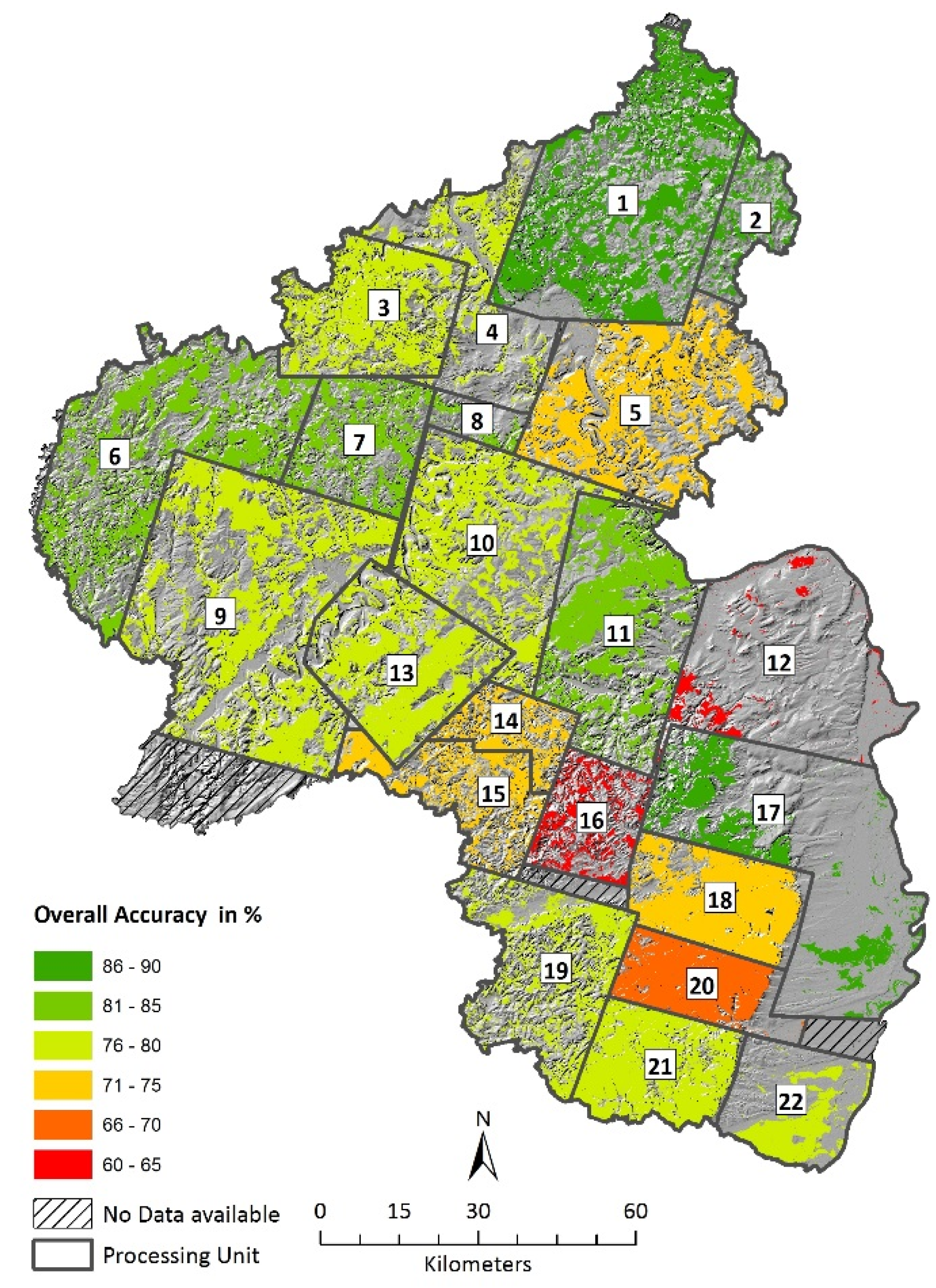
5.3.3. Problem Analysis

The spatially adaptive classification of the five main tree species achieved an overall accuracy within the quality specification of the state forest service, whereas the classification of species and development stage (overall accuracy of 55%) did not fulfill the requirements. However, feedback from expert field evaluations of the derived species and development stage information layer reported high quality and good usability in specific forest districts. As mentioned (see Section 2.2.1), the limitations of satellite data availability precluded classification of the whole study area in one process. Instead, the considered satellite data, representing the phenological stage of foliage development and full foliage had to be processed as 22 individual data stacks. This is viewed as a major limitation to the concept of spatially adaptive classification. However, the advantages in overcoming classifier deficiency emerging from variable ecological growth conditions and management schemes outweigh the restrictions associated with the limited spatial extent of the processing units.

In order to estimate the product quality at a regional scale and to evaluate the effect of fragmenting the study site into 22 processing units, a detailed assessment was performed of the achieved classification accuracies within each unit.

Due to variations in unit size and tree species composition, the amount of validation data was only sufficient for a unit-based accuracy assessment at the species level. Figure 8 shows the overall classification accuracy achieved for each of the 22 processing units at tree species level.

Figure 8. Overall classification accuracy at tree species level for each of the 22 processing units.

Figure 8. Overall classification accuracy at tree species level for each of the 22 processing units.

Compared with the overall classification accuracy of 83.5% for the whole study area, unit-based accuracy ranges from 69% (unit 17) to 87% (units 1 and 17); 16 of the 22 processing units achieve overall accuracies >75%, corresponding to 70.6% of total forested area within the state. A further three processing units obtained accuracies >70%, and only three units had overall accuracies <70%. Nonetheless, Figure 7 shows distinct regional differences in the mapped processing units. To determine the causes of quality deficiencies, Table 5 summarizes the characteristics of each processing unit and their respective accuracies. See Supplementary Information 2 for more details about the proportional coverage of the five main tree species according to the official forest inventory data.

Table 5. Processing unit characteristics and overall classification accuracies.

Processing Unit		Early-Spring Acquisition Period			Summer Acquisition Period			Details		Phenology
ID	Area (km2)	Acquisition date	Sensor	Incidence angle	Acquisition date	Sensor	Incidence angle	Total cloud cover (%)	Forested area (%)	Reported foliage formation (beech)	Delay in days	Acquisition delay in days	OA (%)
17	1593	20/04/2009	S4	17.2	31/08/2005	S5	1.3	0.2	20	13/04/2009	7	1328	87.1
1	1673	24/04/2011	S4	8.3	31/07/2005	S5	19.8	1.9	44	12/04/2011	12	997	86.3
2	315	25/04/2011	S5	29.7	31/07/2005	S5	19.8	0.7	31	12/04/2011	13	998	85.5
6	1510	05/05/2008	S5	20.6	15/07/2008	S5	22.5	12.3	35	30/04/2008	5	–71	82.0
8	137	22/05/2010	S5	25.1	16/08/2009	S5	19.6	0	18	22/04/2010	30	279	81.5
7	553	05/05/2008	S5	20.6	16/08/2009	S5	19.6	12.9	36	30/04/2008	5	–468	81.4
11	1132	18/04/2010	S5	27.7	03/07/2010	S5	21.2	6.3	51	24/04/2010	–6	–76	80.5
3	752	05/05/2008	S5	20.6	16/08/2009	S5	19.6	1	54	30/04/2008	5	–468	79.8
4	755	10/05/2008	S5	14.2	16/08/2009	S5	19.6	0.1	23	21/04/2008	19	–463	79.5
9	1977	05/05/2008	S5	20.6	31/08/2009	S5	4.7	1	41	28/04/2008	7	–483	79.3
22	519	07/04/2010	S5	12.3	14/07/2010	S5	10.8	6.4	32	23/04/2010	–6	–98	79.1
21	575	07/04/2010	S5	12.3	05/09/2009	S5	2.6	1.3	80	19/04/2010	–12	1675	76.9
19	869	10/05/2008	S5	10.8	31/07/2008	S5	19.8	1	36	25/04/2008	15	–82	76.6
10	1108	06/04/2010	RE	3.8	03/07/2006	S5	13.9	0	42	26/04/2010	–20	1373	76.4
13	833	06/04/2010	RE	3.8	07/08/2010	RE	7.6	0	53	22/04/2010	–16	–123	75.9
15	532	06/04/2010	RE	3.8	07/08/2010	S5	22.4	0	43	24/04/2010	–18	–93	74.5
18	611	20/04/2009	S4	17.2	31/08/2005	S5	1.3	0.9	74	13/04/2009	7	1328	73.1
14	287	06/04/2010	RE	3.8	07/08/2010	S5	22.4	0	46	24/04/2010	–18	–93	71.9
5	1294	25/04/2011	S5	29.7	31/07/2008	S5	19.7	1	40	16/04/2011	9	998	70.7
20	459	20/04/2009	S4	17.2	05/09/2009	S5	2.6	3	74	09/04/2009	11	1323	69.1
12	1288	25/05/2009	S5	17.1	05/08/2009	S5	3.4	0.8	5	09/04/2009	46	–72	64.1
16	423	06/04/2010	RE	3.8	07/08/2010	RE	7.6	33	37	25/04/2010	–19	–123	63.3

Table 5. Processing unit characteristics and overall classification accuracies.

Processing Unit		Early-Spring Acquisition Period			Summer Acquisition Period			Details		Phenology
ID	Area (km2)	Acquisition date	Sensor	Incidence angle	Acquisition date	Sensor	Incidence angle	Total cloud cover (%)	Forested area (%)	Reported foliage formation (beech)	Delay in days	Acquisition delay in days	OA (%)
17	1593	20/04/2009	S4	17.2	31/08/2005	S5	1.3	0.2	20	13/04/2009	7	1328	87.1
1	1673	24/04/2011	S4	8.3	31/07/2005	S5	19.8	1.9	44	12/04/2011	12	997	86.3
2	315	25/04/2011	S5	29.7	31/07/2005	S5	19.8	0.7	31	12/04/2011	13	998	85.5
6	1510	05/05/2008	S5	20.6	15/07/2008	S5	22.5	12.3	35	30/04/2008	5	–71	82.0
8	137	22/05/2010	S5	25.1	16/08/2009	S5	19.6	0	18	22/04/2010	30	279	81.5
7	553	05/05/2008	S5	20.6	16/08/2009	S5	19.6	12.9	36	30/04/2008	5	–468	81.4
11	1132	18/04/2010	S5	27.7	03/07/2010	S5	21.2	6.3	51	24/04/2010	–6	–76	80.5
3	752	05/05/2008	S5	20.6	16/08/2009	S5	19.6	1	54	30/04/2008	5	–468	79.8
4	755	10/05/2008	S5	14.2	16/08/2009	S5	19.6	0.1	23	21/04/2008	19	–463	79.5
9	1977	05/05/2008	S5	20.6	31/08/2009	S5	4.7	1	41	28/04/2008	7	–483	79.3
22	519	07/04/2010	S5	12.3	14/07/2010	S5	10.8	6.4	32	23/04/2010	–6	–98	79.1
21	575	07/04/2010	S5	12.3	05/09/2009	S5	2.6	1.3	80	19/04/2010	–12	1675	76.9
19	869	10/05/2008	S5	10.8	31/07/2008	S5	19.8	1	36	25/04/2008	15	–82	76.6
10	1108	06/04/2010	RE	3.8	03/07/2006	S5	13.9	0	42	26/04/2010	–20	1373	76.4
13	833	06/04/2010	RE	3.8	07/08/2010	RE	7.6	0	53	22/04/2010	–16	–123	75.9
15	532	06/04/2010	RE	3.8	07/08/2010	S5	22.4	0	43	24/04/2010	–18	–93	74.5
18	611	20/04/2009	S4	17.2	31/08/2005	S5	1.3	0.9	74	13/04/2009	7	1328	73.1
14	287	06/04/2010	RE	3.8	07/08/2010	S5	22.4	0	46	24/04/2010	–18	–93	71.9
5	1294	25/04/2011	S5	29.7	31/07/2008	S5	19.7	1	40	16/04/2011	9	998	70.7
20	459	20/04/2009	S4	17.2	05/09/2009	S5	2.6	3	74	09/04/2009	11	1323	69.1
12	1288	25/05/2009	S5	17.1	05/08/2009	S5	3.4	0.8	5	09/04/2009	46	–72	64.1
16	423	06/04/2010	RE	3.8	07/08/2010	RE	7.6	33	37	25/04/2010	–19	–123	63.3

To identify the main reasons why the overall accuracy of >85% could only be achieved for three processing units, information about satellite data quality and availability, phenological development, processing unit size and characteristics, available forest information data, forest structure, composition, and ownership as well as the evaluations of the forestry experts were reviewed. Table 5 lists all processing units in descending order of classification accuracy and provides strong explanatory evidence for the low classification accuracies of units 16 and 12. For unit 16, the low overall accuracy of 63.3% is attributed to high cloud cover in the only available satellite scene during the summer acquisition period. For unit 12, the low overall classification accuracy of 64.1% is attributed to low forest cover and corresponding low availability of reference data, combined with the late acquisition date during the spring observation period. Conversely, the combination of significant size and suitable early spring acquisition date, matching the phenological stage of foliage formation, lead to very high overall classification accuracies of 86.3% and 87.1% for processing units 1 and 17, respectively. Yet, especially the high overall classification result of processing unit 8 (81.5%) is not compatible with this scheme. Unit 8 has an area of only 137 km² and there is a phenological mismatch in the satellite data acquisition date during the early spring observation period. A detailed survey of the available forest information data and high spatial -resolution aerial imagery revealed that the high classification accuracy is driven only by the tree species distribution in this limited area. The area, a small tributary valley of the Moselle River, is characterized by an exceptionally high degree of deciduous forest cover (around 75%); therefore, the classification accuracy is not comparable with other processing units.

Considering the final evaluation survey, the experience from the data preprocessing, the preliminary study [18], as well as the feedback from the forest survey experts, the following were identified as main factors influencing the spatially adaptive classification:

(1)

Phenology: Spectral separability of deciduous tree species can be substantially increased if the combined satellite observations capture the important phenological stages of foliage formation and fully developed foliage [18,26,29,82,83]. To ensure high mapping quality of forest information layers, the required satellite observations should be acquired within the optimum phenological time-windows.

(2)

Spatial extent of processing unit: To compensate climatic- and management-dependent gradients in forest site conditions, the use of a spatially adaptive classification approach seems to be a feasible strategy. However, the spatial extent of the processing unit should be large enough to ensure sufficient reference data for the classification process and thereby the best possible spatial adaptation to the forest characteristics.

Consequently, the quality of the derived forest information layers depends strongly on the quality, consistency, and availability of satellite data. Furthermore, this demonstrates that spatially adaptive selection of reference samples offers only a partial solution to the problem of achieving consistent classification results across larger areas. It overcomes inconsistencies in the class descriptors emerging from variable ecological conditions and management schemes and can handle varying availability of reference data within a study area. However, the spatially adaptive organization of the available reference data does not consider the additional requirement that for optimum phenological timing of multi-temporal satellite datasets. Our spatially adaptive scheme should be extended and improved to also provide appropriate and consistent reference data across areas with different phenological development.

6. Conclusions

Satellite-derived forest information layers were integrated with operational forest survey methods to support the development of an innovative forest management system for the federal state of Rhineland-Palatinate, Germany. Using multi-phenological satellite data, the following forest information mapping layers were derived: forest/non-forest, forest type, tree species distribution, and tree species with their development stages. All training data were automatically drawn from the official forestry data base of the state forest administration. The core concept further included a radiometric pre-processing chain with correction of relief-induced illumination artifacts, which is an essential prerequisite for coping with topographically complex terrain. The classification strategy used satellite observations from two distinctly different phenological stages (springtime leaf emergence vs. summertime optimum development of the tree layer) and employed a spatially adaptive version of a maximum likelihood classifier [18]. Three of the four resulting forest information layers (FIL 1–FIL 3) achieved mapping accuracies suitable for an immediate integration into the operational forest inventory methods, whereas the fourth forest information layer (FIL 4: tree species and associated development stages) requires further improvements (see Figure 9). However, in areas where an optimum set of satellite images was available, forest practitioners and survey experts also confirmed the potential usefulness of FIL 4 for preparing and conducting terrestrial surveys. Consequently, also FIL 4 will be considered as an additional input to the operational forest inventory concept, provided that satellite systems with suitable acquisition capacities become available.

The results of this pilot project confirm that the operational requirements for mapping accuracies can, in principle, be fulfilled. However, the state-wide mapping experiment also revealed that the required accuracy largely depends on the availability of satellite observations which cover large areas within the optimum phenological time-windows (April/May and July/August). Particularly Sentinel-2, with its optimized acquisition strategy, wide-swath observation geometry, high spatial resolution, and extended band set, is a prime candidate to overcome the data-dependent limitations identified so far, and thereby form the backbone of a future EO-supported forest observatory at federal state level. We therefore conclude that the expected improvements in satellite availability will be a milestone towards integrating EO products into operational forest inventory and monitoring systems.

Figure 9. Conceptual layout of operational forest information layers derived of the conclusion of this study.

Figure 9. Conceptual layout of operational forest information layers derived of the conclusion of this study.

Based on the results of this study, it is also envisaged that state-wide forest information layers may be integrated into the official geodata infrastructure of RLP to be shared with further potential users; such as the state survey or nature conservation agencies (see Figure 9). Additionally, it has been decided to continue with the acquisition of high quality airborne LiDAR data in the forthcoming years. It can therefore be expected that consistent crown height information will soon be available for the complete federal state area, and can then be integrated as an additional classification layer to further improve the FIL products.

References

1. Food and Agricultural Organization of the United Nations. Global Forest Land-use Change 1990–2005; Food and Agricultural Organization of the United Nations: Rome, Italy, 2012. [Google Scholar]
2. Hansen, M.C.; Potapov, P.V.; Moore, R.; Hancher, M.; Turubanova, S.A.; Tyukavina, A.; Thau, D.; Stehman, S.V.; Goetz, S.J.; Loveland, T.R.; et al. High-resolution global maps of 21st-century forest cover change. Science 2013, 342, 850–853. [Google Scholar] [CrossRef] [PubMed]
3. Foley, J.A.; DeFries, R.; Asner, G.P.; Barford, C.; Bonan, G.; Carpenter, S.R.; Chapin, F.S.; Coe, M.T.; Daily, G.C.; Gibbs, H.K.; et al. Global consequences of land use. Science 2005, 309, 570–574. [Google Scholar] [CrossRef] [PubMed]
4. McRoberts, R.E.; McWilliams, W.H.; Reams, G.A.; Schmidt, T.L.; Jenkins, J.C.; O’Neill, K.P.; Miles, P.D.; Brand, G.J. Assessing sustainability using data from the forest inventory and analysis program of the United States forest service. J. Sustain. Forest. 2004, 18, 23–46. [Google Scholar] [CrossRef]
5. UNFCCC (United Nations Framework Convention on Climate Change). The Kyoto Protocol to the Convention on Climate Change; Climate Change Secretariat: Bonn, Germany, 1998. [Google Scholar]
6. Glowka, L.; Burhenne-Guilmin, F.; Synge, H.; McNeely, J.A.; Gündling, L. A Guide to the Convention on Biological Diversity; IUCN Environmental Law Center & IUCN Biodiversity Programme: Gland, Switzerland, 1994. [Google Scholar]
7. Forest Europe. Oslo Ministerial Decision: European Forest 2020; Forest Europe: Oslo, Norway, 2011. [Google Scholar]
8. McDonald, G.T.; Lane, M.B. Converging global indicators for sustainable forest management. For. Policy Econ. 2004, 6, 63–70. [Google Scholar] [CrossRef]
9. Bolte, A.; Eisenhauer, D.-R.; Ehrhart, H.-P.; Groß, J.; Hanewinkel, M.; Kölling, C.; Profft, I.; Rohde, M.; Röhe, P.; Amereller, K. Klimawandel und Forstwirtschaft—Übereinstimmungen und Unterschiede bei der Einschätzung der Anpassungsnotwendigkeiten und Anpassungsstrategien der Bundesländer. Landbauforschung 2009, 59, 269–278. [Google Scholar]
10. Franklin, S.E. Remote Sensing for Sustainable Forest Management; Lewis Publishers: Boca Raton, FL, USA; London, UK; New York, NY, USA; Washington, DC, USA, 2001. [Google Scholar]
11. Andersson, F.O.; Feger, K.-H.; Hüttl, R.F.; Kräuchi, N.; Mattsson, L.; Sallnäs, O.; Sjöberg, K. Forest ecosystem research—Priorities for Europe. For. Ecol. Manag. 2000, 132, 111–119. [Google Scholar] [CrossRef]
12. Linke, J.; Betts, M.; Lavigne, B.; Franklin, S.E. Introduction: Structure, function, and change of forest landscapes. In Understanding Forest Disturbance and Spatial Pattern. Remote Sensing and GIS Approaches; Wulder, M.A., Franklin, S.E., Eds.; CRC Press/Taylor & Francis Group: Boca Raton, FL, USA, 2006; pp. 1–22. [Google Scholar]
13. Boyd, D.S.; Danson, F.M. Satellite remote sensing of forest resources: Three decades of research development. Prog. Phys. Geogr. 2005, 29, 1–26. [Google Scholar] [CrossRef]
14. Holmgren, P.; Thuresson, T. Satellite remote sensing for forestry planning a review. Scand. J. For. Res. 1998, 13, 90–110. [Google Scholar] [CrossRef]
15. Kempeneers, P.; Sedano, F.; Seebach, L.; Strobl, P.; San-Miguel-Ayanz, J. Data fusion of different spatial resolution remote sensing images applied to forest-type mapping. IEEE T. Geosci. Remote 2011, 49, 4977–4986. [Google Scholar] [CrossRef]
16. Pekkarinen, A.; Reithmaier, L.; Strobl, P. Pan-European forest/non-forest mapping with Landsat ETM+ and Corine land cover 2000 data. ISPRS J. Photogramm. Remote Sens. 2009, 64, 171–183. [Google Scholar] [CrossRef]
17. Holopainen, M.; Vastaranta, M.; Liang, X.; Hyyppä, J.; Jaakkola, A.; Kankare, V. Estimation of forest stock and yield using lidar data. In Remote Sensing of Natural Resources; Wang, G., Weng, Q., Eds.; CRC Press Taylor & Francis Group: Boca Ratom, FL, USA, 2014; pp. 259–290. [Google Scholar]
18. Stoffels, J.; Mader, S.; Hill, J.; Werner, W.; Ontrup, G. Satellite-based stand-wise forest cover type mapping using a spatially adaptive classification approach. Eur. J. For. Res. 2012, 131, 1071–1089. [Google Scholar] [CrossRef]
19. LWaldG. Landeswaldgesetz Rheinland-Pfalz (Forest Act Rhineland-Palatinate); LwaldG: Rhineland-Palatinate, Germany, 2000. [Google Scholar]
20. Peerenboom, H.G.; Ontrup, G.; Böhmer, O. Weiterentwicklung der Forsteinrichtung in Rheinland-Pfalz. Forst Holz 2003, 58, 728–731. [Google Scholar]
21. Diemer, C.; Lucaschewski, I.; Spelsberg, G.; Tomppo, E.; Pekkarien, A. Integration of Terrestrial Forest Sample Plot Data, Map Information and Satellite Data: An Operational Multisource-Inventory Concept., Fusion of Earth Data: Merging Point Measurements, Raster Maps and Remotely Sensed Images., Sophia Antipolis, France; Ranchin, T., Wald, L., Eds.; SEE/URISCA, Nice: Sophia Antipolis, France, 2000; pp. 485–497. [Google Scholar]
22. Vohland, M.; Stoffels, J.; Hau, C.; Schüler, G. Remote sensing techniques for forest parameter assessment: Multispectral classification and linear spectral mixture analysis. Silva Fenn. 2007, 41, 441–456. [Google Scholar] [CrossRef]
23. Gauer, J. Waldökologische Naturräume Deutschlands. In Forstliche Wuchsgebiete und Wuchsbezirke. Mitteilungen des Vereins für Forstliche Standortskunde und Forstpflanzenzüchtung; Gauer, J., Aldinger, E., Eds.; Henkeldruck: Stuttgart, Germany, 2005; Volume 43, pp. 13–17. [Google Scholar]
24. PEFC-Arbeitsgruppe Rheinland-Pfalz. 3. Regionaler Waldbericht Rheinland-Pfalz; Programme for the Endorsement of Forest Certification Schemes: Trippstadt, Germany, 2010. [Google Scholar]
25. Wolff, B.; Erhard, M.; Holzhausen, M.; Kuhlow, T. Das Klima in den Forstlichen Wuchsgebieten und Wuchsbezirken Deutschlands; Kommissionsverlag Buchhandlung Max Widebusch: Hamburg, Germany, 2003. [Google Scholar]
26. Dymond, C.C.; Mladenoff, D.J.; Radeloff, V.C. Phenological differences in tasseled cap indices improve deciduous forest classification. Remote Sens. Environ. 2002, 80, 460–472. [Google Scholar] [CrossRef]
27. Wolter, P.T.; Townsend, P.A.; Sturtevant, B.R. Estimation of forest structural parameters using 5 and 10 meter SPOT-5 satellite data. Remote Sens. Environ. 2009, 113, 2019–2036. [Google Scholar] [CrossRef]
28. Wolter, P.T.; Mladenoff, D.J.; Host, G.E.; Crow, T.R. Improved forest classification in northern lake states using multi-temporal Landsat imagery. Photogramm. Eng. Remote Sens. 1995, 61, 1129–1143. [Google Scholar]
29. Schriever, J.R.; Congalton, R.G. Evaluating seasonal variability as an aid to cover-type mapping from Landsat thematic mapper data in the northeast. Photogramm. Eng. Remote Sens. 1995, 61, 321. [Google Scholar]
30. Kuemmerle, T.; Radeloff, V.C.; Perzanowski, K.; Hostert, P. Cross-border comparison of land cover and landscape pattern in Eastern Europe using a hybrid classification technique. Remote Sens. Environ. 2006, 103, 449–464. [Google Scholar] [CrossRef]
31. Polgar, C.A.; Primack, R.B. Leaf-out phenology of temperate woody plants: From trees to ecosystems. New Phytol. 2011, 191, 926–941. [Google Scholar] [CrossRef] [PubMed]
32. Rötzer, T.; Chmielewski, F.-M. Phenological maps of Europe. Clim. Res. 2001, 18, 249–257. [Google Scholar] [CrossRef]
33. Rötzer, T.; Grote, R.; Pretzsch, H. The timing of bud burst and its effect on tree growth. Int. J. Biometeorol. 2004, 48, 109–118. [Google Scholar] [CrossRef] [PubMed]
34. DWD Climate Data Center (CDC). Eintrittsdaten Phänologischer Phasen, Sofortmelder Wildwachsende Pflanzen. 2015. Available online: http:///ftp-cdc.dwd.de/pub/CDC/observations_germany/phenology/annual_reporters/wild/ (accessed on 29 May 2015).
35. Wesołowski, T.; Rowiński, P. Timing of bud burst and tree-leaf development in a multispecies temperate forest. For. Ecol. Manag. 2006, 237, 387–393. [Google Scholar] [CrossRef]
36. Spotimage—Astrum-Geo. Spot Image, Resolutions and Spectral Modes. Available online: http://www2.astrium-geo.com/files/pmedia/public/r451_9_resolutionspectralmodes_uk_sept2010.pdf (accessed on 1 October 2014).
37. Blackbridge. Satellite Imagery Product Specifications. Available online: http://blackbridge.com/rapideye/upload/RE_Product_Specifications_ENG.pdf (accessed on 1 October 2014).
38. Bundesministerium für Verbraucherschutz Ernährung und Landwirtschaft. Die Zweite Bundeswaldinventur—Das Wichtigste in Kürze; Bundesministerium für Verbraucherschutz, Ernährung und Landwirtschaft, Referat Öffentlichkeitsarbeit: Bonn, Germany, 2004. [Google Scholar]
39. Landesforsten Rheinland-Pfalz. Naturnahe Waldbewirtschaftung—Qualifizieren—Dimensionieren. Available online: http://www.wald-rlp.de (accessed on 8 August 2008).
40. St-Onge, B.; Treitz, P.; Wulder, M.A. Tree and canopy height estimation with scanning lidar. In Remote Sensing of Forest Environments; Wulder, M.A., Franklin, S.E., Eds.; Springer: New York, NY, USA, 2003; pp. 489–509. [Google Scholar]
41. Immitzer, M.; Atzberger, C.; Koukal, T. Tree species classification with random forest using very high spatial resolution 8-band Worldview-2 satellite data. Remote Sens. 2012, 4, 2661–2693. [Google Scholar] [CrossRef]
42. Wulder, M.A. Optical remote-sensing techniques for the assessment of forest inventory and biophysical parameters. Prog. Phys. Geogr. 1998, 22, 449–476. [Google Scholar] [CrossRef]
43. Hill, J.; Diemer, C.; Udelhoven, T. A Local Correlation approach for the fusion of image bands with different spatial resolutions. Bull. Soc. Fr. Photogramm. Télédétect. 2003, 169, 26–34. [Google Scholar]
44. De Boissezon, H.; Laporterie-Déjean, F. Evaluations thématiques et statistiques de cinq algorithmes de fusion p/xs sur des simulations d’images pleiades-hr. Bull. Soc. Fr. Photogramm. Télédétect. 2003, 169, 83–99. [Google Scholar]
45. Verbyla, D.L.; Hammond, T.O. Conservative bias in classification accuracy assessment due to pixel-by-pixel comparison of classified images with reference grids. Int. J. Remote Sens. 1995, 16, 581–587. [Google Scholar] [CrossRef]
46. Townshend, R.G.; Justice, C.O.; Gurney, C.; McManus, J. The impact of misregistration on change detection. IEEE T. Geosci. Remote 1992, 30, 1054–1060. [Google Scholar] [CrossRef]
47. Hill, J.; Mehl, W. Geo- und radiometrische Aufbereitung multi- und hyperspektraler Daten zur Erzeugung langjähriger kalibrierter Zeitreihen. Photogramm. Fernerkund. Geoinf. 2003, 2003, 7–14. [Google Scholar]
48. Radeloff, V.; Hill, J.; Mehl, W. Forest Mapping from Space—Enhanced Satellite Data Processing by Spectral Mixture Analysis and Topographic Corrections; European Commission ECSC-EC-EAEC: Brüssel, Luxemburg, 1997; p. 90. [Google Scholar]
49. Ekstrand, S. Landsat TM-based forest damage assessment: Correction for topographic effects. Photogramm. Eng. Remote Sens. 1996, 62, 151–162. [Google Scholar]
50. Dorren, L.K.A.; Maier, B.; Seijmonsbergen, A.C. Improved Landsat-based forest mapping in steep mountainous terrain using object-based classification. For. Ecol. Manag. 2003, 183, 31–46. [Google Scholar] [CrossRef]
51. Hale, S.R.; Rock, B.N. Impact of topographic normalization on land-cover classification accuracy. Photogramm. Eng. Remote Sens. 2003, 69, 785–791. [Google Scholar] [CrossRef]
52. Itten, K.; Meyer, P.; Kellenberger, T.; Leu, R.; Sandmeier, S.; Bittner, P.; Seidel, K. Correction of the Impact of Topography and Atmosphere on Landsat-TM Forest Mapping of Alpine Regions; Remote Sensing Series, Volume 18; RSL, University of Zürich: Zürich, Switzerland, 1992. [Google Scholar]
53. Hill, J.; Mehl, W.; Radeloff, V.C. Improved Forest Mapping by Combining Corrections of Atmospheric and Topographic Effects in Landsat TM Imagery. Göteborg, Sweden, 6–8 June 1995; Askne, J., Ed.; pp. 143–151.
54. Conese, C.; Gilabert, M.A.; Maselli, F.; Bottai, L. Topographic normalization of tm scenes through the use of an atmospheric correction method and digital terrain models. Photogramm. Eng. Remote Sens. 1993, 59, 1745–1753. [Google Scholar]
55. Hill, J.; Sturm, B. Radiometric correction of multi-temporal thematic mapper data for the use in agricultural land-cover classification and vegetation monitoring. Int. J. Remote Sens. 1991, 12, 1471–1491. [Google Scholar] [CrossRef]
56. Tanré, D.; Deroo, C.; Duhaut, P.; Hermann, M.; Mocrette, J.J.; Perbos, J.; Deschamps, P.Y. Description of a computer code to simulate the satellite signal in the solar spectrum—The 5 s code. Int. J. Remote Sens. 1990, 11, 659–668. [Google Scholar] [CrossRef]
57. Song, C.; Woodcock, C.E.; Seto, K.C.; Pax-Lenney, M.; Macomber, S.A. Classification and change detection using Landsat TM data: When and how to correct atmospheric effects? Remote Sens. Environ. 2001, 75, 230–244. [Google Scholar] [CrossRef]
58. Meyer, P.; Itten, K.I.; Kellenberger, T.; Sandmeier, S.; Sandmeier, R. Radiometric corrections of topographically induced effects on Landsat TM data in an alpine environment. ISPRS J. Photogramm. Remote Sens. 1993, 48, 17–28. [Google Scholar] [CrossRef]
59. Buddenbaum, H.; Schlerf, M.; Hill, J. Classification of coniferous tree species and age classes using hyperspectral data and geostatistical methods. Int. J. Remote Sens. 2005, 26, 5453–5465. [Google Scholar] [CrossRef]
60. Bauer, M.E.; Burk, T.E.; Ek, A.R.; Coppin, P.R.; Lime, S.D.; Walsh, T.A.; Walters, D.K.; Befort, W.; Heinzen, D.F. Satellite inventory of Minnesota forest resources. Photogramm. Eng. Remote Sens. 1994, 60, 287–298. [Google Scholar]
61. Reese, H.M.; Lillesand, T.M.; Nagel, D.E.; Stewart, J.S.; Goldmann, R.A.; Simmons, T.E.; Chipman, J.W.; Tessar, P.A. Statewide land cover derived from multiseasonal Landsat TM data. A retrospective of the WISCLAND project. Remote Sens. Environ. 2002, 82, 224–237. [Google Scholar] [CrossRef]
62. Campbell, J.B. Spatial correlation effects upon accuracy of supervised classification of land cover. Photogramm. Eng. Remote Sens. 1981, 47, 355–363. [Google Scholar]
63. Gong, P.; Howarth, P.J. An assessment of some factors, influencing multispectral land-cover classification. Photogramm. Eng. Remote Sens. 1990, 56, 597–603. [Google Scholar]
64. Ball, G.H.; Hall, D.J. ISODATA, a Novel Method of Data Analysis and Pattern Classification; Stanford Research Institute: Menlo Park, CA, USA, 1965. [Google Scholar]
65. Kuntz, S.; Schmeer, E.; Jochum, M.; Smith, G. Towards an European land cover monitoring service and high-resolution layers. In Land Use and Land Cover Mapping in Europe; Manakos, I., Braun, M., Eds.; Springer: Dordrecht, The Netherlands, 2014; Volume 18, pp. 43–52. [Google Scholar]
66. Brus, D.J.; Hengeveld, G.M.; Walvoort, D.J.J.; Goedhart, P.W.; Heidema, A.H.; Nabuurs, G.J.; Gunia, K. Statistical mapping of tree species over Europe. Eur. J. For. Res. 2012, 131, 145–157. [Google Scholar] [CrossRef]
67. Schuck, A.; Päivinen, R.; Häme, T.; van Brusselen, J.; Kennedy, P.; Folving, S. Compilation of a European forest map from Portugal to the Ural Mountains based on Earth observation data and forest statistics. For. Policy Econ. 2003, 5, 187–202. [Google Scholar] [CrossRef]
68. Mathys, L.; Guisan, A.; Kellenberger, T.W.; Zimmermann, N.E. Evaluating effects of spectral training data distribution on continuous field mapping performance. ISPRS J. Photogramm. Remote Sens. 2009, 64, 665–673. [Google Scholar] [CrossRef]
69. Swain, P.H.; Davis, S.M. Fundamentals of Pattern Recognition in Remote Sensing; McGraw Hill Book Company: New York, NY, USA, 1978; pp. 136–185. [Google Scholar]
70. Stehman, S.V. Selecting and interpreting measures of thematic classification accuracy. Remote Sens. Environ. 1997, 62, 77–89. [Google Scholar] [CrossRef]
71. Foody, G.M. Status of land cover classification accuracy assessment. Remote Sens. Environ. 2002, 80, 185–201. [Google Scholar] [CrossRef]
72. Story, M.; Congalton, R.G. Accuracy assessment: A user’s perspective. Photogramm. Eng. Remote Sens. 1986, 52, 397–399. [Google Scholar]
73. Congalton, R.G. A review of assessing the accuracy of classifications of remotely sensed data. Remote Sens. Environ. 1991, 37, 35–46. [Google Scholar] [CrossRef]
74. Cohen, J. A coefficient of agreement for nominal scales. Educ. Psychol. Meas. 1960, 20, 37–46. [Google Scholar] [CrossRef]
75. Hudson, W.D.; Ramm, C.W. Correct formulation of the kappa coefficient of agreement. Photogramm. Eng. Remote Sens. 1987, 53, 421–422. [Google Scholar]
76. European Environment Agency. Gio Land (GMES/Copernicus Initial Operations Land) High-resolution Layers (HRLs)—Summary of Product Specifications; European Environment Agency: Copenhagen, Denmark, 2013. [Google Scholar]
77. Probeck, M.; Ramminger, G.; Herrmann, D.; Gomez, S.; Häusler, T. European forest monitoring approaches. In Land Use and Land Cover Mapping in Europe; Manakos, I., Braun, M., Eds.; Springer: Dordrecht, The Netherlands, 2014; Volume 18, pp. 89–114. [Google Scholar]
78. Thünen-Institut. Dritte Bundeswaldinventur—Ergebnisdatenbank. Available online: https://bwi.info (accessed on 18 December 2014).
79. Bundesministerium für Ernährung und Landwirtschaft. Bundeswaldinventur. Available online: https://www.bundeswaldinventur.de/ (accessed on 18 December 2014).
80. Stehman, S.V.; Czaplewski, R.L. Design and analysis for thematic map accuracy assessment—An application of satellite imagery. Remote Sens. Environ. 1998, 64, 331–344. [Google Scholar] [CrossRef]
81. Congalton, R.G.; Green, K. Assessing the Accuracy of Remotely Sensed Data: Principles and Practices; CRC Press: New York, NY, USA, 1999. [Google Scholar]
82. Hill, R.A.; Wilson, A.K.; George, M.; Hinsley, S.A. Mapping tree species in temperate deciduous woodland using time-series multi-spectral data. Appl. Veg. Sci. 2010, 13, 86–99. [Google Scholar] [CrossRef]
83. Mickelson, J.G. Delineating forest canopy species in the northeastern United States using multi-temporal tm imagery. Photogramm. Eng. Remote Sens. 1998, 64, 891. [Google Scholar]