
Utilizing HyspIRI Prototype Data for Geological Exploration Applications: A Southern California Case Study

Abstract
:
1. Introduction
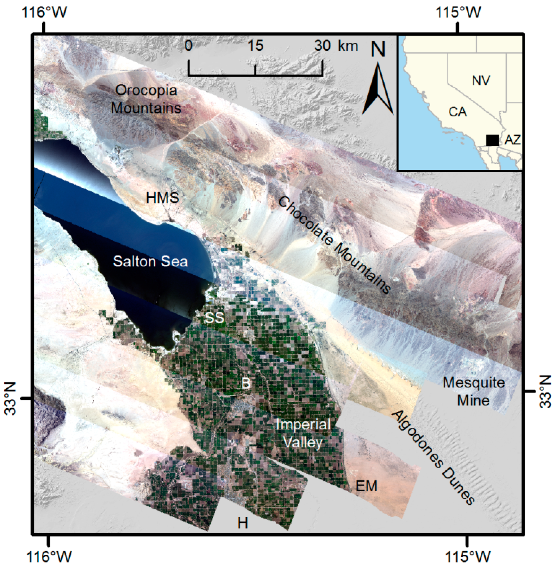
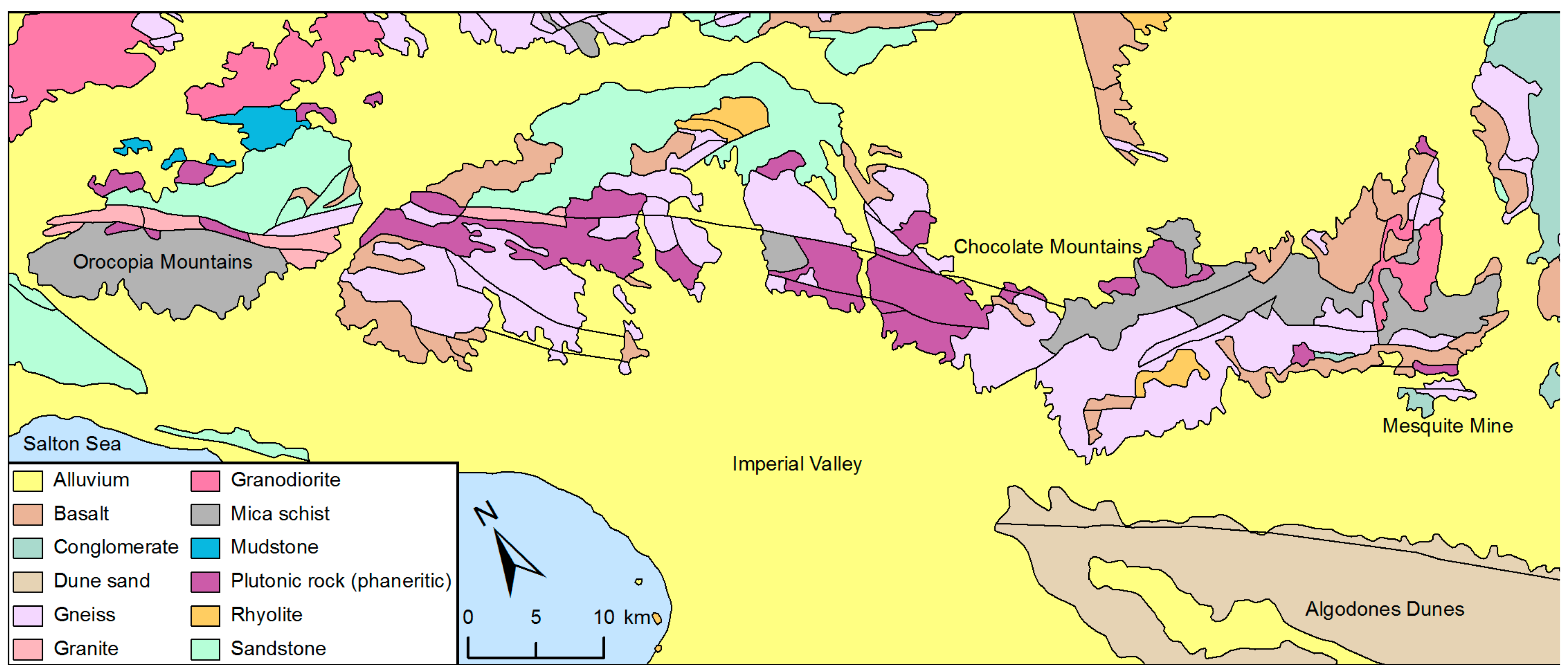
2. Geologic Setting
3. Materials and Methods
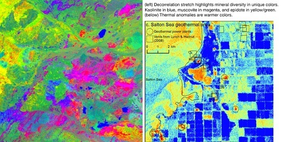
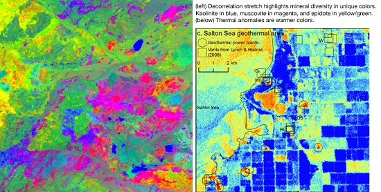
3.1. VSWIR Decorrelation Stretch to Quickly Identify Alteration
3.2. VSWIR Data for Mineral Mapping
3.3. TIR Decorrelation Stretch to Quickly Identify Lithology
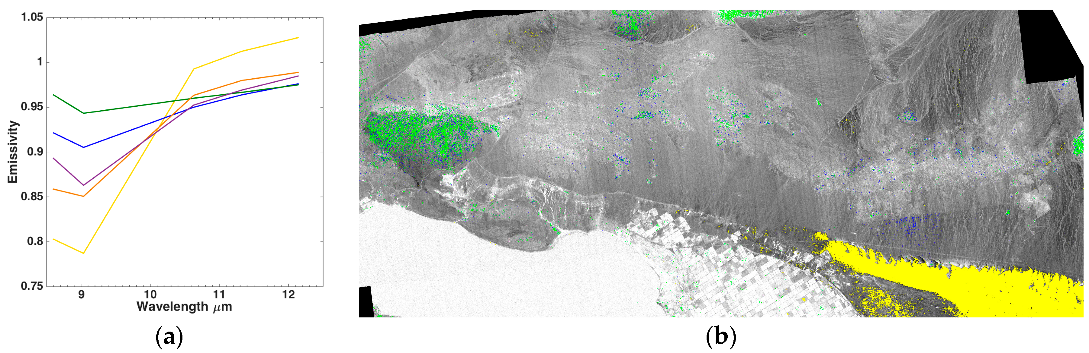
3.4. TIR Emissivity Data for Lithologic Mapping
3.5. TIR Data for Thermal Anomaly Identification
4. Results
4.1. VSWIR Decorrelation Stretch to Quickly Identify Alteration
4.2. VSWIR Data for Hydrothermal Alteration Mapping
4.3. TIR Decorrelation Stretch to Quickly Identify Lithology
4.4. TIR Emissivity Data for Lithologic Mapping
4.5. TIR Data for Thermal Anomaly Identification
5. Discussion
5.1. Hydrothermal Alteration Mapping
5.2. Lithologic Mapping
5.3. Thermal Anomaly Mapping
6. Conclusions
Acknowledgments
Author Contributions
Conflicts of Interest
Abbreviations
| ASTER | Advanced Spaceborne Thermal Emission and Reflectance Radiometer |
| AVIRIS | Advanced Visible/Infrared Imaging Specrometer |
| DCS | decorrelation stretch |
| HyspIRI | Hyperspectral Infrared Imager |
| MASTER | MODIS/ASTER Airborne Simulator |
| TIR | Thermal Infrared |
| VSWIR | Visible and Short-Wave Infrared |
References
- Sabins, F.F. Remote sensing for mineral exploration. Ore Geol. Rev. 1999, 14, 157–183. [Google Scholar] [CrossRef]
- Yamaguchi, Y.; Kahle, A.B.; Tsu, H.; Kawakami, T.; Pniel, M. Overview of Advanced Spaceborne Thermal Emission and Reflection Radiometer (ASTER). IEEE Trans. Geosci. Remote Sens. 1998, 36, 1062–1071. [Google Scholar] [CrossRef]
- Pearlman, J.S.; Barry, P.S.; Segal, C.C.; Shepanski, J.; Beiso, D.; Carman, S.L. Hyperion, a space-based imaging spectrometer. IEEE Trans. Geosci. Remote Sens. 2003, 41, 1160–1173. [Google Scholar] [CrossRef]
- Van der Meer, F.D.; van der Werff, H.M.A.; van Ruitenbeek, F.J.A.; Hecker, C.A.; Bakker, W.H.; Noomen, M.F.; van der Meijde, M.; Carranza, E.J.M.; de Smeth, J.B.; Woldai, T. Multi- and hyperspectral geologic remote sensing: A review. Int. J. Appl. Earth Obs. Geoinf. 2012, 14, 112–128. [Google Scholar] [CrossRef]
- Hewson, R.D.; Cudahy, T.J.; Huntington, J.F. Geologic and alteration mapping at Mt Fitton, South Australia, using ASTER satellite-borne data. In Proceedings of the 2001 IEEE Geoscience and Remote Sensing Symposium, Sydney, Australia, 9–13 July 2001; pp. 724–726.
- Rowan, L.C.; Mars, J.C. Lithologic mapping in the Mountain Pass, California area using Advanced Spaceborne Thermal Emission and Reflection Radiometer (ASTER) data. Remote Sens. Environ. 2003, 84, 350–366. [Google Scholar] [CrossRef]
- Mars, J.C.; Rowan, L.C. Spectral assessment of new ASTER SWIR surface reflectance data products for spectroscopic mapping of rocks and minerals. Remote Sens. Environ. 2010, 114, 2011–2025. [Google Scholar] [CrossRef]
- Zhang, X.; Pamer, M.; Duke, N. Lithologic and mineral information extraction for gold exploration using ASTER data in the south Chocolate Mountains (California). ISPRS J. Photogramm. Remote Sens. 2007, 62, 271–282. [Google Scholar] [CrossRef]
- Rowan, L.C.; Hook, S.J.; Abrams, M.J.; Mars, J.C. Mapping hydrothermally altered rocks at Cuprite, Nevada, using the Advanced Spaceborne Thermal Emission and Reflection Radiometer (ASTER), a new satellite-imaging system. Econ. Geol. 2003, 98, 1019–1027. [Google Scholar] [CrossRef]
- Bedini, E. Mineral mapping in the Kap Simpson complex, central east Greenland, using Hymap and ASTER remote sensing data. Adv. Space Res. 2011, 47, 60–73. [Google Scholar] [CrossRef]
- Middleton, E.M.; Ungar, S.G.; Mandl, D.J.; Ong, L.; Frye, S.W.; Campbell, P.E.; Landis, D.R.; Young, J.P.; Pollack, N.H. The Earth Observing One (EO-1) satellite mission: Over a Decade in Space. IEEE J. Sel. Top. Appl. Earth Obs. Remote Sens. 2013, 6, 243–256. [Google Scholar] [CrossRef]
- Green, R.O.; Pavri, B.E.; Chrien, T.G. On-orbit radiometric and spectral calibration characteristics of EO-1 Hyperion derived with an underflight of AVIRIS and in situ measurements at Salar de Arizaro, Argentina. IEEE Trans. Geosci. Remote Sens. 2003, 41, 1194–1203. [Google Scholar] [CrossRef]
- Bergeron, M.; Hollinger, A.; Staenz, K.; Maszkiewicz, M.; Neville, R.A.; Qian, S.E.; Goodenough, D.G. Hyperspectral environment and resource observer (HERO) mission. Can. J. Remote Sens. 2008, 34, S1–S11. [Google Scholar] [CrossRef]
- Guanter, L.; Kaufmann, H.; Segl, K.; Foerster, S.; Rogass, C.; Chabrillat, S.; Kuester, T.; Hollstein, A.; Rossner, G.; Chlebek, C.; et al. The EnMAP spaceborne imaging spectroscopy mission for earth observation. Remote Sens. 2015, 7, 8830–8857. [Google Scholar] [CrossRef]
- Matsunaga, T.; Iwasaki, A.; Tsuchida, S.; Tanii, J.; Kashimura, O.; Nakamura, R.; Yamamoto, H.; Tachikawa, T.; Rokugawa, S. Current status of Hyperspectral Imager Suite (HISUI). In Proceedings of the 2014 IEEE International Geoscience and Remote Sensing Symposium (IGARSS), Quebec, QC, Canada, 13–18 July 2014.
- Lopinto, E.; Ananasso, C. The Prisma Hyperspectral Mission. Available online: http://www.earsel.org/symposia/2013-symposium-Matera/proceedings.php (accessed on 4 January 2016).
- Lee, C.M.; Cable, M.L.; Hook, S.J.; Green, R.O.; Ustin, S.L.; Mandl, D.J.; Middleton, E.M. An introduction to the NASA Hyperspectral Infrared Imager (HyspIRI) mission and preparatory activities. Remote Sens. Environ. 2015, 167, 6–19. [Google Scholar] [CrossRef]
- AVIRIS Web Site. Available online: http://aviris.jpl.nasa.gov (accessed on 16 February 2016).
- MASTER Web Site. Available online: http://masterweb.jpl.nasa.gov (accessed on 16 February 2016).
- Jennings, C.W.; Strand, R.G.; Rogers, T.H. Geologic Map of California, Scale 1:750,000; California Division of Mines and Geology: Piscataway, NJ, USA, 1977. [Google Scholar]
- Jennings, O.P. Geologic Map of California: Salton Sea Sheet, Scale 1:250,000; California Division of Mines and Geology: Sacramento, CA, USA, 1967. [Google Scholar]
- Bjornstad, S.; Alm, S.; Huang, W.; Tiedeman, A.; Frazier, L.; Page, C.; Sabin, A.; Veazey, D. An Update on Geothermal Energy Resource Investigations, Chocolate Mountains Aerial Gunnery Range, Imperial Valley, California. Trans. Geotherm. Resour. Counc. 2011, 35, 713–720. [Google Scholar]
- New Gold Inc. Technical Report on the Mesquite Mine, Imperial County, California, USA; NI 43–101 Report; Roscoe Postle Associates Inc.: Toronto, ON, Canada, 2014. [Google Scholar]
- Jacobsen, C.E.; Grove, M.; Vućić, A.; Pedrick, J.N.; Ebert, K.A. Exhumation of the Orocopia Schist and associated rocks of southeastern California: Relative Roles of Erosion, Synsubduction Tectonic Denudation, and Middle Cenozoic Extension. Geol. Soc. Am. Spec. Pap. 2007, 419, 1–37. [Google Scholar]
- Norris, R.M.; Norris, K.S. Algodones Dunes of southeastern California. Geol. Soc. Am. Bull. 1961, 72, 605–620. [Google Scholar] [CrossRef]
- Lynch, D.K.; Hudnut, K.W.; Adams, P.M. Development and growth of recently-exposed fumarole fields near Mullet Island, Imperial County, California. Geomorphology 2013, 195, 27–44. [Google Scholar] [CrossRef]
- Lynch, D.K.; Hudnut, K.W. The Wister mud pot lineament: Southeastward Extension or Abandoned Strand of the San Andreas Fault? Bull. Seismol. Soc. Am. 2008, 98, 1720–1729. [Google Scholar] [CrossRef]
- Reath, K.A.; Ramsey, M.S. Exploration of geothermal systems using hyperspectral thermal infrared remote sensing. J. Volcanol. Geotherm. Res. 2013, 265, 27–38. [Google Scholar] [CrossRef]
- Tratt, D.M.; Young, S.J.; Lynch, D.K.; Buckland, K.N.; Johnson, P.D.; Hall, J.L.; Westberg, K.R.; Polak, M.L.; Kasper, B.P.; Qian, J. Remotely sensed ammonia emission from fumarolic vents associated with a hydrothermally active fault in the Salton Sea Geothermal Field, California. J. Geophys. Res. 2011, 116, D21308. [Google Scholar] [CrossRef]
- Schmitt, A.K.; Martin, A.; Stockli, D.F.; Farley, K.A.; Lovera, O.M. (U-Th)/He Zircon and archaeological ages for a late prehistoric eruption in the Salton Trough (California, USA). Geology 2013, 41, 7–10. [Google Scholar] [CrossRef]
- Wright, H.M.; Vazquez, J.A.; Champion, D.E.; Calvert, A.T.; Mangan, M.T.; Stelten, M.; Cooper, K.M.; Herzig, C.; Schriener, A. Episodic Holocene eruption of the Salton Buttes rhyolites, California, from paleomagnetic, U-Th, and Ar/Ar dating. Geochem. Geophys. Geosyst. 2015, 16, 1198–1210. [Google Scholar] [CrossRef]
- Brothers, D.S.; Driscoll, N.W.; Kent, G.M.; Harding, A.J.; Babcock, J.M.; Baskin, R.L. Tectonic evolution of the Salton Sea inferred from seismic reflection data. Nat. Geosci. 2009, 2, 581–584. [Google Scholar] [CrossRef]
- McGuire, J.J.; Lohman, R.B.; Catchings, R.D.; Rymer, M.J.; Goldman, M.R. Relationships among seismic velocity, metamorphism, and seismic and aseismic fault slip in the Salton Sea Geothermal Field region. J. Geophys. Res. Solid Earth 2015, 120, 2600–2615. [Google Scholar] [CrossRef]
- Wei, S.J.; Avouac, J.P.; Hudnut, K.W.; Donnellan, A.; Parker, J.W.; Graves, R.W.; Helmberger, D.; Fielding, E.; Liu, Z.; Cappa, F.; et al. The 2012 Brawley swarm triggered by injection-induced aseismic slip. Earth Planet. Sci. Lett. 2015, 422, 115–125. [Google Scholar] [CrossRef]
- Thompson, D.R.; Gao, B.C.; Green, R.O.; Roberts, D.A.; Dennison, P.E.; Lundeen, S.R. Atmospheric correction for global mapping spectroscopy: ATREM Advances for the HyspIRI Preparatory Campaign. Remote Sens. Environ. 2015, 167, 64–77. [Google Scholar] [CrossRef]
- Orthorectified HyspIRI Preparatory Campaign Products. Available online: ftp://popo.jpl.nasa.gov/2013_HyspIRI_Prep_Data/AVIRIS_HyspIRI_Simulated_Data_Products.readme (accessed on 21 December 2015).
- Grigsby, S.P.; Hulley, G.C.; Roberts, D.A.; Scheele, C.; Ustin, S.L.; Alsina, M.M. Improved surface temperature estimates with MASTER/AVIRIS sensor fusion. Remote Sens. Environ. 2015, 167, 53–63. [Google Scholar] [CrossRef]
- Littlefield, E.F.; Calvin, W.M. Geothermal exploration using imaging spectrometer data over Fish Lake Valley, Nevada. Remote Sens. Environ. 2014, 140, 509–518. [Google Scholar] [CrossRef]
- Clark, R.N.; Swayze, G.A.; Wise, R.; Livo, E.; Hoefen, T.; Kokaly, R.; Sutley, S.J. USGS Digital Spectral Library Splib06a; U.S. Geological Survey: Reston, VA, USA, 2007. [Google Scholar]
- Kruse, F.A.; Taranik, J.V.; Coolbaugh, M.; Michaels, J.; Littlefield, E.F.; Calvin, W.M.; Martini, B.A. Effect of reduced spatial resolution on mineral mapping using imaging spectrometry-examples using Hyperspectral Infrared Imager (HyspIRI)-simulated data. Remote Sens. 2011, 3, 1584–1602. [Google Scholar] [CrossRef] [Green Version]
- Calvin, W.M.; Littlefield, E.F.; Kratt, C. Remote sensing of geothermal-related minerals for resource exploration in Nevada. Geothermics 2015, 53, 517–526. [Google Scholar] [CrossRef]
- Vaughan, R.G.; Hook, S.J.; Calvin, W.M.; Taranik, J.V. Surface mineral mapping at Steamboat Springs, Nevada, USA, with multi-wavelength thermal infrared images. Remote Sens. Environ. 2005, 99, 140–158. [Google Scholar] [CrossRef]
- Hewson, R.D.; Cudahy, T.J.; Mizuhiko, S.; Ueda, K.; Mauger, A.J. Seamless geological map generation using ASTER in the broken Hill-Curnamona province of Australia. Remote Sens. Environ. 2005, 99, 159–172. [Google Scholar] [CrossRef]
- Rowan, L.C.; Mars, J.C.; Simpson, C.J. Lithologic mapping of the Mordor, NT, Australia ultramafic complex by using the Advanced Spaceborne Thermal Emission and Reflection Radiometer (ASTER). Remote Sens. Environ. 2005, 99, 105–126. [Google Scholar] [CrossRef]
- Rowan, L.C.; Schmidt, R.G.; Mars, J.C. Distribution of hydrothermally altered rocks in the Reko Diq, Pakistan mineralized area based on spectral analysis of ASTER data. Remote Sens. Environ. 2006, 104, 74–87. [Google Scholar] [CrossRef]
- Coolbaugh, M.F.; Kratt, C.; Fallacaro, A.; Calvin, W.M.; Taranik, J.V. Detection of geothermal anomalies using Advanced Spaceborne Thermal Emission and Reflection Radiometer (ASTER) thermal infrared images at Bradys Hot Springs, Nevada, USA. Remote Sens. Environ. 2007, 106, 350–359. [Google Scholar] [CrossRef]
- Rockwell, B.W.; Hofstra, A.H. Identification of quartz and carbonate minerals across northern Nevada using ASTER thermal infrared emissivity data—Implications for geologic mapping and mineral resource investigations in well-studied and frontier areas. Geosphere 2008, 4, 218–246. [Google Scholar] [CrossRef]
- Hook, S.J.; Dmochowski, J.E.; Howard, K.A.; Rowan, L.C.; Karlstrom, K.E.; Stock, J.M. Mapping variations in weight percent silica measured from multispectral thermal infrared imagery—Examples from the Hiller Mountains, Nevada, USA and Tres Virgenes-La Reforma, Baja California Sur, Mexico. Remote Sens. Environ. 2005, 95, 273–289. [Google Scholar] [CrossRef]


| HyspIRI [17] | ASTER Channel [6] | ASTER Wavelength [6] | MASTER 1 | MASTER-TES Processed |
|---|---|---|---|---|
| 7.35 | -- | -- | -- | -- |
| -- | -- | -- | 7.8 | -- |
| 8.28 | 10 | 8.3 | 8.18 | -- |
| 8.63 | 11 | 8.65 | 8.62 | 8.6 |
| 9.07 | 12 | 9.1 | 9.06 | 9.03 |
| -- | -- | -- | 9.67 | -- |
| -- | -- | -- | 10.10 | -- |
| 10.53 | 13 | 10.6 | 10.59 | 10.63 |
| 11.33 | 14 | 11.3 | 11.33 | 11.32 |
| 12.05 | -- | -- | 12.12 | 12.1 |
| -- | -- | -- | 12.86 | -- |
© 2016 by the authors; licensee MDPI, Basel, Switzerland. This article is an open access article distributed under the terms and conditions of the Creative Commons by Attribution (CC-BY) license (http://creativecommons.org/licenses/by/4.0/).
Share and Cite
Calvin, W.M.; Pace, E.L. Utilizing HyspIRI Prototype Data for Geological Exploration Applications: A Southern California Case Study. Geosciences 2016, 6, 11. https://0-doi-org.brum.beds.ac.uk/10.3390/geosciences6010011
Calvin WM, Pace EL. Utilizing HyspIRI Prototype Data for Geological Exploration Applications: A Southern California Case Study. Geosciences. 2016; 6(1):11. https://0-doi-org.brum.beds.ac.uk/10.3390/geosciences6010011
Chicago/Turabian StyleCalvin, Wendy M., and Elizabeth L. Pace. 2016. "Utilizing HyspIRI Prototype Data for Geological Exploration Applications: A Southern California Case Study" Geosciences 6, no. 1: 11. https://0-doi-org.brum.beds.ac.uk/10.3390/geosciences6010011