Article

A Multispectral Bayesian Classification Method for Increased Acoustic Discrimination of Seabed Sediments Using Multi-Frequency Multibeam Backscatter Data

by
Timo C. Gaida
1,*,
Tengku Afrizal Tengku Ali
1,2,
Mirjam Snellen
1,3,
Alireza Amiri-Simkooei
1,
Thaiënne A. G. P. Van Dijk
3 and
Dick G. Simons
1
1
Acoustics Group, Faculty of Aerospace Engineering, Delft University of Technology, 2629 HS Delft, The Netherlands
2
Department of Survey Science and Geomatics, Universiti Teknologi MARA Perlis, Arau 02600, Malaysia
3
Department of Applied Geology and Geophysics, Deltares, 3508 AL Utrecht, The Netherlands
*
Author to whom correspondence should be addressed.
Submission received: 7 November 2018 / Revised: 27 November 2018 / Accepted: 29 November 2018 / Published: 4 December 2018
(This article belongs to the Special Issue Geological Seafloor Mapping)

Abstract

:
Multi-frequency backscatter data collected from multibeam echosounders (MBESs) is increasingly becoming available. The ability to collect data at multiple frequencies at the same time is expected to allow for better discrimination between seabed sediments. We propose an extension of the Bayesian method for seabed classification to multi-frequency backscatter. By combining the information retrieved at single frequencies we produce a multispectral acoustic classification map, which allows us to distinguish more seabed environments. In this study we use three triple-frequency (100, 200, and 400 kHz) backscatter datasets acquired with an R2Sonic 2026 in the Bedford Basin, Canada in 2016 and 2017 and in the Patricia Bay, Canada in 2016. The results are threefold: (1) combining 100 and 400 kHz, in general, reveals the most additional information about the seabed; (2) the use of multiple frequencies allows for a better acoustic discrimination of seabed sediments than single-frequency data; and (3) the optimal frequency selection for acoustic sediment classification depends on the local seabed. However, a quantification of the benefit using multiple frequencies cannot clearly be determined based on the existing ground-truth data. Still, a qualitative comparison and a geological interpretation indicate an improved discrimination between different seabed environments using multi-frequency backscatter.

1. Introduction

Multibeam echosounders (MBESs) have become the most valuable tool for seafloor mapping providing high-resolution bathymetry and acoustic backscatter datasets [1]. Various classification methods, employing MBES bathymetry, backscatter, and their second order moments, have been developed to characterize seabeds or riverbeds in the last two decades [2]. They aim at maximizing the performance in discriminating between different seabed environments or sediment types. Acoustic backscatter strength is the most common feature used in seabed classification [2]. The backscatter strength is dependent on the composition of the seabed, angle of incidence, and acoustic frequency [3]. Seabed roughness, volume heterogeneity, bulk density, as well as discrete scatterers and sediment layering that contribute to the seabed composition all affect the backscatter strength [3,4]. The frequency dependence of backscatter strength is caused by three main factors: (i) the relationship between seabed roughness and acoustic wavelength [5], (ii) the dominant scattering regime, i.e., Rayleigh or geometrical scattering, which is dependent on the acoustic wavelength and particle size [6,7,8], and (iii) the contribution of volume scattering influenced by the signal penetration [9,10,11]. In several lab and field experiments, in which the influence of varying frequencies on the backscatter strength was studied, it was shown that specific sediment types have different acoustic responses at different frequencies (e.g., [4,7,12,13,14]). In field measurements, Urick [13] observed no significant frequency dependency for rough sediments (sedimentary rocks), whereas the scattering from soft sediments (silt) increased slightly with increasing frequencies from 10 to 80 kHz. Jackson et al. [12] observed an increasing frequency dependency from very fine sediments (sandy silt: − 0.2 dB per octave) to fine sediments (medium sand: 2 db/oct) followed by a decrease for coarser sediments (fine gravel: 1.5 db/oct) for a frequency range from 20 to 85 kHz. Tank measurements carried out by Ivakin & Sessarego [7] demonstrated the frequency dependence of scattering for coarse and medium sand within a frequency range from 150 kHz to 2 MHz. Hefner et al. [14] showed, in a tank experiment, higher frequency dependency for a sandy bottom (fine) than for a sandy bottom covered with shell fragments (coarse) within a frequency range from 200 to 500 kHz. These studies indicate that, for most sediment types and frequencies, a frequency dependency of the backscatter strength is to be expected. In general, it is observed that finer sediments (e.g., sand) show a higher sensitivity to different acoustic frequencies than coarser sediments (e.g., gravel, shells, or boulders). As a next level of complexity, where the layering of sediments is considered, a study by Williams et al. [4] demonstrated the significant influence of a thin mud layer (in parts exceeding 10 cm) covering a well-sorted medium sand on scattering at different frequencies. Comparing the scattering at a well-sorted medium sand with the mud/sand surface layer, they showed that the scattering of the sorted medium sand was attributed to the surface interface roughness, whereas volume scattering dominated for the mud/sand layer for frequencies from 20 to 150 kHz. For frequencies higher than 200 kHz volume and roughness scattering could not explain the observed scattering strength. This is an indication for a change in the scattering regime (Rayleigh to geometrical scattering). All of the above shows the complex interaction between acoustics and the seabed. More acoustic lab and field experiments need to be carried out to capture the multispectral acoustic response of the entire variety of sediments. Still, these results provide promising opportunities to overcome ambiguities in the relationship between monochromatic backscatter and sediment properties by utilizing multiple frequencies [15,16].
The first acquisition and analysis of multi-frequency backscatter acquired with a co-located MBES operating at 70–100 kHz and 200–400 kHz was carried out in 2015 [17]. The study shows clear variations in the shape of the angular response as well as in the scattering strength at different frequencies. Since commercial multi-frequency MBESs were not available for the marine acoustic remote sensing community, potential benefits of using multiple frequencies for acoustic seabed classification (ASC) could not be fully elaborated. Typically, the backscatter data are collected at one specific frequency or in a narrow band around the central frequency (monochromatic). As a result, acquiring backscatter at multiple frequencies would require running exactly the same line multiple times, which leads to inefficient and complicated data acquisition. Recently, R2Sonic has developed a broadband MBES (R2Sonic 2026) that allows for collecting spatially and temporarily co-located multispectral backscatter data using a single system. This MBES emits a series of signals between 90 and 450 kHz on a ping-by-ping basis. In Brown et al. [18], the first multispectral backscatter dataset acquired with a single MBES system (R2Sonic 2026) in the Bedford Basin, Canada, was employed and analyzed. The preliminary results of this study indicate benefits for an improved understanding of seabed characteristics by using multispectral backscatter.
In terrestrial remote sensing, the processing and classification of multispectral data are well established. Acquiring data across a wide spectrum of electromagnetic wavelengths has significantly increased the discrimination power of the classification routines [19]. Using multispectral backscatter in a marine environment with the aim of seabed classification requires an appropriate data processing to account for the frequency dependency of environmental and sonar specific variables. Furthermore, an objective and automatic classification technique that is capable of revealing and combining the acoustic information about seabed characteristics at different frequencies is needed to produce a single classification map.
In this study, the Bayesian method for unsupervised seabed classification, which has already been successfully employed in previous studies to single frequency MBES datasets (e.g., [16,20,21]), is extended for the classification of multispectral backscatter data. The method accounts for the intrinsic natural variability of the backscatter strength [22] by assuming that the histogram of the measured backscatter per beam corresponds to a sum of Gaussian distributions, where each Gaussian corresponds to a distinct seabed type [20]. The technique considers thus the backscatter strength per beam (or incident angle). As a result, by considering a constant incident angle, the backscatter strength is only dependent on frequency and seabed properties, providing a promising opportunity for multispectral backscatter. One of the most important features of the Bayesian method is the statistical calculation of the number of classes that can be acoustically distinguished. Here, we use the method to evaluate and quantify the benefits of using multiple frequencies for acoustic seabed classification.
The extended method is tested on three multispectral MBES datasets (100, 200 and 400 kHz) acquired in the Bedford Basin, Canada, in 2016 and 2017 and in the Patricia Bay, Canada, in 2016. The dataset were provided by R2Sonic as a part of an R2Sonic multispectral challenge in 2018. In this manuscript, the acoustic data processing is described in detail with a particular focus on the frequency dependent environmental (i.e., absorption) and sonar specific variables (e.g., beam width) to provide relative backscatter strength per frequency and incident angle.

2. Study Area and Dataset
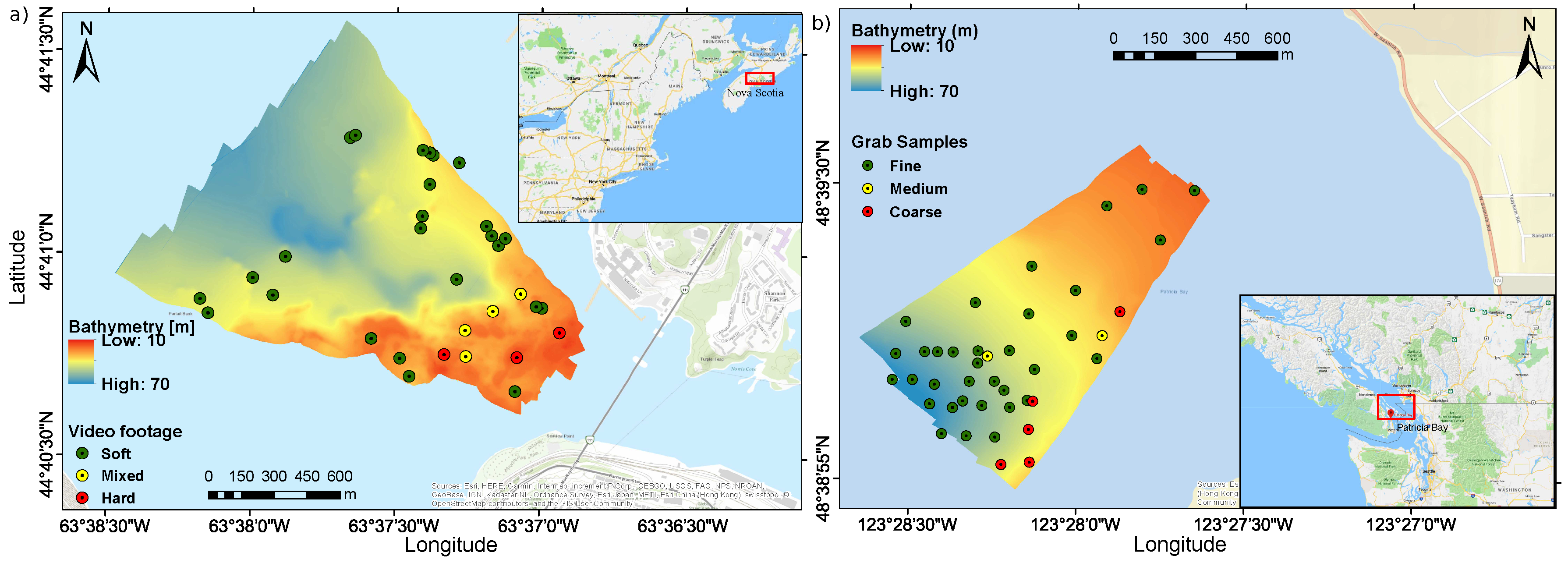
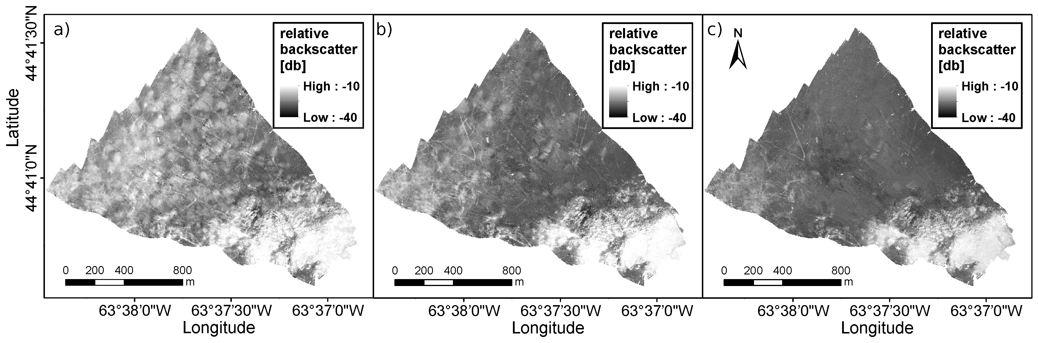
2.1. Bedford Basin

Two MBES datasets were acquired in the Bedford Basin, Halifax, Nova Scotia, by a broadband MBES (R2Sonic 2026) in March 2016 and May 2017, with a total of 15 and 13 lines, respectively, and approximately 50% overlap. The data were collected at three different frequencies (100, 200, and 400 kHz). The MBES data cover an area of approximately 1.84 km2, and the water depth ranges from 13 to 85 m (Figure 1a). Further, georeferenced video footage was collected within the survey area in March 2016 using a drop-down underwater camera frame fitted with a Sub-C underwater camera (SubC Imaging, Clarenville, NL, Canada) and lights [18]. The seabed, visible on the video footage, is categorized into three distinct classes: soft, mixed, and hard. “Hard” represents all areas where the entire area is covered with boulders, shells, or gravel. “Mixed” displays areas where a mixture of soft sediments and boulders is observed. “Soft” comprises all areas where only muddy and sandy sediments are present. A finer distinction of the category “soft” is not pursued because of the following reasons: (i) a clear distinction between mud, silt, or fine sand is not feasible on the basis of the existing video footage, and (ii) the amount and consistency of benthic flora and fauna or gas releases vary significantly. Overall the study area comprises sediment types ranging from bedrock to silt with underlying harder substrate. Different types of benthic flora and fauna are visible in the video footages as well. As reported in [18], the deeper area consists of soft mud partly covered with various benthic flora. In addition, the presence of biogenic gas and the disposal of dredge spoils were observed [23]. Close to the harbor (SE in Figure 1a), the area comprises a mixture of hard substrate such as bedrock, corals, and boulders with attached epifauna.

2.2. Patricia Bay

The third MBES dataset was acquired in Patricia Bay, Canada, in November 2016 using the same R2Sonic 2026 MBES as in the Bedford Basin. The MBES data covers an area of approximately 0.96 km2, and the water depth ranges from 20 to 70 m (Figure 1b). A total of 8 lines were surveyed with approximately 50% overlap. Surficial sediment descriptions are available from a number of grab samples collected during two previous surveys in 2005 and 2006 [24]. The geographical locations of the samples were extracted from a digitalized map in Arc GIS. The samples were classified after the Folk and Wentworth scheme as fine sand (FS), muddy sand (mS), sand (S), gravelly sand (gS), and sandy cobble (sC) in [24]. Here, we reclassify the sediment samples into three categories: fine (FS and mS), medium (S), and coarse (gS and sC). This is done because the use of two different classification schemes generates discrepancies in the interpretation of the sediment samples. The Patricia Bay area was acoustically sensed and classified into a sediment map in a previous study [24]. In essence, Patricia Bay has a complex seabed with a wide range of depths, seabed slopes, and sediment types.

2.3. Multispectral Data

The MBES backscatter is stored as a single value of backscatter intensity per beam representing the return level at the bottom detection point and as a time-series per beam representing the scatter pixels [25]. In this study, the backscatter intensities per beam are considered. The operating settings were tuned to achieve full coverage for all frequencies yielding to varying acquisition parameters in the employed datasets. The system settings such as transmit power, gain, and pulse length are all accessible to the user or predefined in automatic acquisition modes. Table 1 shows the technical characteristics of the R2Sonic 2026 MBES and some parameters used during the acquisition. The raw data is extracted from the generic sensor format (GSF) files and further processed using Matlab scripts developed in this study.

3. Theory and Method

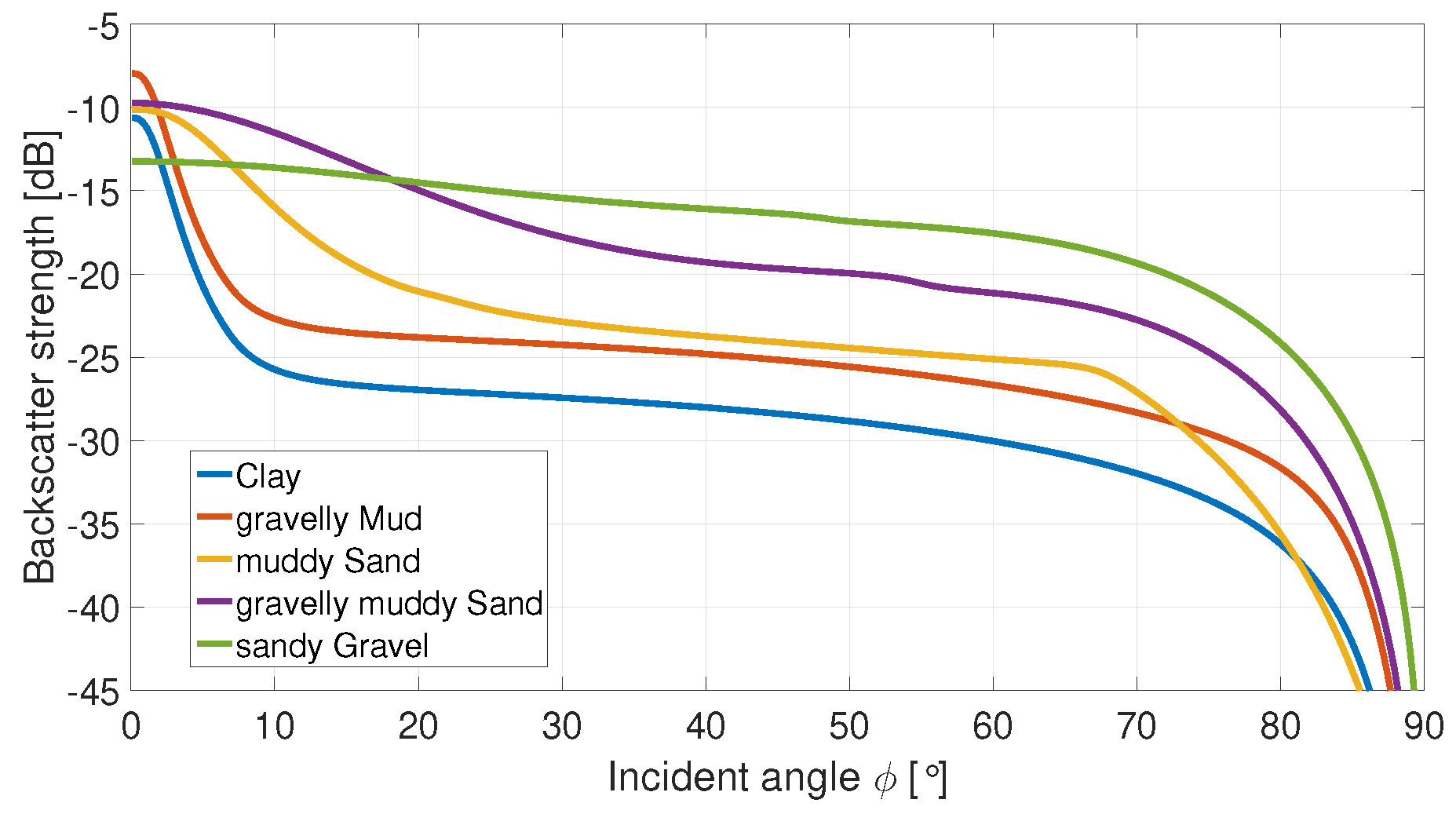
3.1. Acoustic Theory

Backscatter strength B S (in dB re 1 m per m 2 ) is dependent on the composition of the seafloor, the angle of incidence ϕ on the seabed, and the acoustic frequency f [3]. Thus, the backscatter strength provides an indication of the seafloor properties [26]. However, before any useful information can be extracted from the received acoustic echo level E L at the MBES, an appropriate processing is necessary to account for the measurement configuration, seawater properties and the hardware and software settings of the sonar. The terms affecting B S f ( ϕ ) are expressed by the sonar equation (modified from [27,28])
B S f ( ϕ ) = E L S L B P T ( f , θ T ) + T L P G S H ( f ) B P R ( f , θ R ) 10 l o g ( A )
where S L is the source level (in dB re 1 μ Pa at 1 m), modulated by the transmission directivity pattern B P T as a function of f and the transmission angle θ T with respect to the sonar axis. P G (in dB) is the receiver gain applied by the receiver electronics, S H (in dB re 1 V/ μ Pa) is the transducer sensitivity with respect to f, and B P R is the directivity pattern at reception expressed as a function of f and the receiving angle θ R with respect to the sonar axis. B S f is defined per m 2 and derived from the target strength T S = B S f + 10 l o g ( A ) (in dB re 1 m2) via the ensonified footprint area A. The transmission loss T L depends on the water conditions and the travel distance R of the signal to the seabed. It can be written as
T L = 2 α R + 40 l o g ( R )
where α is the absorption coefficient depending on the temperature, salinity, acidity, pressure, and f. The second term in Equation (2) accounts for the energy loss of the signal due to geometrical spreading. A is affected not only by the sonar characteristics but also by the seabed morphology, i.e., the across-track slope ϵ y and along-track slope ϵ x (radians). The ensonified footprint area in the pulse limited regime A p and in the beam limited regime A b , respectively, are expressed by [29]
A p = Ω t x R c τ e f f 2 sin ( ϕ f l ϵ y ) cos ( ϵ x )
and
A b = R 2 Ω t x Ω r x
where c is the sound speed in water, τ e f f is the effective pulse length, and ϕ f l is the incident angle with respect to nadir and a flat seabed. Ω t x and Ω r x are the beam opening angles (representing the 3 dB width of the main lobe) for transmission and reception and can be approximated for a continuous line array with length L and equally spaced transducer elements by [30]
Ω ( θ R , T ) = λ L 1 cos ( θ R , T )
where λ is the wavelength of the transmitted signal given by λ = c / f . The term 1 / cos ( θ R , T ) in Equation (5) describes the increase of the beam opening angle with increasing steering angle θ due to the reduced projected line array length. Considering a constant array length, the beam width changes with varying frequency. Furthermore, the incident angle with respect to the actual seabed ϕ can be calculated from ϕ f l (degrees) according to [29]
cos ( ϕ ) = sin ( 90 ϕ f l ) + cos ( 90 ϕ f l ) ϵ y 1 + ϵ x 2 + ϵ y 2 .
The incident angle correction assigns to each backscatter measurement the true incident angle. In environments with a rough seabed morphology, this correction is essential for seabed classification using backscatter data.
The sonar equation (Equation (1)) allows for the theoretical extraction of the absolute backscatter strength from the received signal of the MBES. However, the necessary variables and parameters might not be available from the sonar producer or measured sufficiently accurately. Even though all variables are properly documented, the conversion from analog to digital data and vice versa at reception and transmission often exhibits a discrepancy between the design and actual hardware implementation. In addition, aging of the MBES components might change the sensitivity of the system hardware over time [28]. In such a case frequently performed relative or absolute calibrations of the MBES systems using natural reference areas or a calibrated singlebeam echosounder can be conducted [31,32]. If no calibration is performed, the backscatter data is considered as uncalibrated data. Still, as long as the relative variation of backscatter strength with respect to varying sediment types and incident angles are preserved within the processing, seabed classification can also be applied.

3.2. Acoustic Data Processing Applied to the R2Sonic 2026

No absolute or relative calibration is applied to the used R2Sonic 2026 MBES. Here, the data processing aims to reveal physical reasonable relative backscatter strength per incident angle. Following Equation (1), the received echo level E L is corrected for the receiver gain P G and the actual source level S L , where the directivity pattern B P R f is already considered; in addition, a correction term is used to account for the difference between the requested and actual source level. R2Sonic MBESs compensate for the transmission loss T L already during the acquisition. However, for the current study, the absorption coefficient α and the spreading coefficient loss term used by the MBES are replaced with physical reasonable values according to Equation (2). The α is estimated using the model of Francois and Garrison [33,34] and subsequently integrated over the depth. The required environmental variables of the water column (temperature, pressure, and salinity) are obtained from measured CTD profiles and a pH value of 8 is assumed. The R2Sonic MBES stores backscatter intensities in digitized pressure units with an unknown scaling caused by uncalibrated sensors. First, the extracted values are converted to decibels. Furthermore, a frequency response correction term is added to the received signal intensity to compensate for the sensitivity of the transducer S H f per frequency (see Equation (1)). The frequency response calculations are a theoretical approximation based on the measured transducer characteristics. In addition, the received signal is compensated for the ensonified footprint area A according to Equations (1), (3), and (4). The beam widths for the three frequencies are displayed in Table 1. In the pulse-limited regime, the calculation of the footprint area A p requires the effective pulse length τ e f f (see Equation (3)). It differs from the nominal pulse length τ n due to the applied trapezoid filter aiming to suppress spectral leakage. In this study, it is assumed that the given receiver bandwidth B stored in the datagrams represents the width of the main lobe of the time series signal in the frequency domain at reception. Considering this assumption, τ e f f can be calculated by τ e f f = 1 / B (Table 1). This results in a τ e f f of 133 μ m, a decrease of 12% compared to τ n . The required across-track ϵ y and along-track slopes ϵ x are calculated from the bathymetric data via a moving window of 50 pings with respect to the heading of the vessel using a 2D finite difference method. Finally, the true incident angle ϕ is calculated by considering the along- and across-track slopes using Equation (6). All levels are shifted by 100 dB. This has no effect on the classification. The value is selected to bring the backscatter values to levels that are typical for marine sediments.

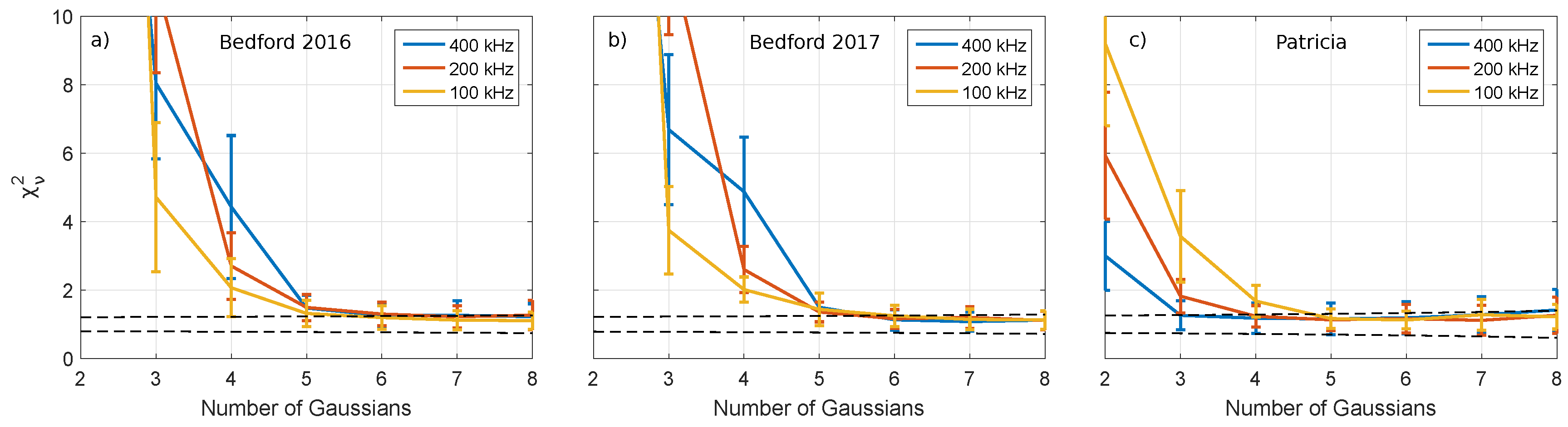
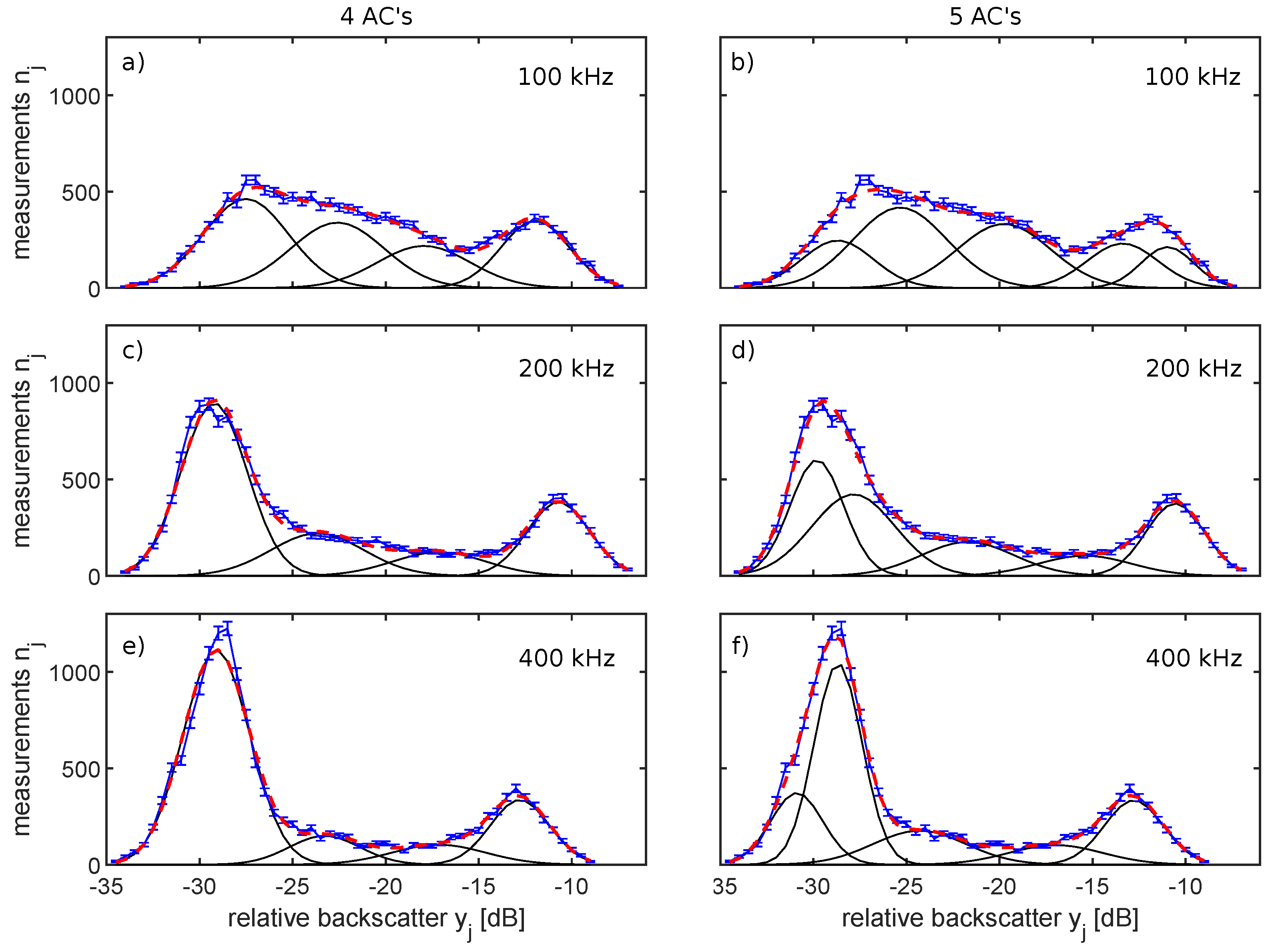
3.3. Bayesian Method

The Bayesian method for sediment classification employed in this paper was first developed in [20], where a detailed description of the theory is given, and developed further by [29]. This section provides an overview of the main concepts and the processing steps taken to generate the acoustic class maps from monochromatic backscatter datasets (Step 1, Figure 2).
Measured backscatter strengths are affected by random fluctuations of the acoustic interaction with the seabed [22] and thus can be considered as a random variable with a certain mean and standard variation. According to the central limit theorem, measured backscatter strengths per beam, which are determined as the average over backscatter from the scatter pixels within a beam (backscatter time series), can be assumed to follow a Gaussian distribution [20]. A scatter pixel represents the instantaneously ensonified area of the seafloor by the transmitted pulse of the MBES, i.e., the signal footprint. If the frequency and angle of incidence are constant, the backscatter strength is dependent on the seabed properties. Thus, if the survey area contains m different sediment types, the backscatter histogram for a selected beam can be represented by a combination of m Gaussian distributions. The modeled backscatter histogram per beam can be expressed as the summation of the m Gaussian distributions according to
f ( y j | x ) = k = 1 m c k exp ( y j y ¯ k ) 2 2 σ y k 2
with y j the jth backscatter value in the histogram ( j = 1 , , M with M the total number of bins in the histogram). x is the vector containing the unknown parameters: x = ( y ¯ 1 , , y ¯ m ; σ y 1 , , σ y m ; c 1 , , c m ) with y ¯ k the means, σ y k the standard deviations, and c k the strengths of the Gaussian distributions. The unknown parameters are determined by maximizing the match between the modeled and the measured histogram in a least squared sense [20]. To solve the non-linear least squares problem, the trust-region-reflective algorithm is used. This algorithm is a trust-region method and is based on the interior-reflective Newton method [35,36]. To determine the optimal number of Gaussians, the Chi-square χ 2 goodness of fit test can be used, where χ 2 is defined as
χ 2 = j = 1 M ( n j f ( y j | x ) 2 σ j 2
and where n j denotes the number of measurements per bin of the aforementioned histogram. For the random variable n j , a Poisson distribution is postulated. The variances σ j 2 are thus equal to n j . The goodness of fit statistic is χ 2 distributed with ν = M 3 m degrees of freedom. The goodness of fit criterion is then further defined as the reduced- χ 2 statistic ( χ ν 2 = χ 2 / ν ) , having a value close to 1 for a good fit. For large ν , the reduced- χ 2 statistic can be approximated by a normal distribution with a mean of 1 and standard deviation of 2 / ν . That means that, if the value of m reaches 1 ± 2 / ν , it follows that this m is considered as the number of seafloor types that can be discriminated in the survey area based on the backscatter data. To increase the robustness of the estimation of the optimal number of Gaussians, the χ 2 -test is applied to a range of beam angles (incident angles). The outer beams are preferably utilized for fitting the Gaussians. First of all, larger incident angles include more scatter pixels per area, lowering the Gaussian’s standard deviation, and consequently provide increased geoacoustic resolution. Second, the incident angles between 30 ° and 70 ° provide the most discrimination potential [5].
The actual classification is based on the Bayes decision rule. In this case, m states or hypotheses, indicated as H k with k = 1 , , m , exist. These hypotheses correspond to the m seafloor types present in the surveyed area. In the following, the Bayesian decision rule for multiple hypotheses is used to define which hypothesis is accepted, i.e.,
accept H k if max { f ( y j | H i ) P ( H i ) } = f ( y j | H k ) P ( H k )
where P ( H i ) is the a priori probability of hypothesis H i with i = 1 , , m . Considering that the measurements are taken for the first time, all hypotheses are equally likely, which results in P ( H i ) = 1 / m . The decision rule is then simplified to
accept H k if max { f ( y j | H i ) } = f ( y j | H k ) .
Therefore, the hypothesis that maximizes the likelihood f ( y j | H ) is selected for observation y j . The intersections of the m Gaussians have thus to be determined, which results in m non-overlapping acceptance regions A k defining the so-called acoustic classes (ACs). The boundaries of the ACs are determined for a certain number of reference angles (mostly outer beams). The reference angles are selected based on three requirements: (1) providing most consistent results in terms of the location of the Gaussian distributions per dataset, (2) offering high discrimination power (30 ° to 70 ° ), and (3) containing less noisy data. Based on the percentage distribution of the ACs at the reference angles, the ACs are assigned to the backscatter data at all considered angles (mostly 10 ° to 60 ° ).
The Bayes decision rule enables one to calculate the probabilities of correct and incorrect decisions β k , i . The overlap between the Gaussian distributions represents the probability of incorrect decisions (i.e., misclassification). Statistically, β k , i denotes the probability that H k is true but H i is chosen and can be expressed as
β k , i = A i f ( y | H k ) d y .
The values of β k , i are contained in the so-called decision matrix and can be used to evaluate the probability of (mis)classification. If k = i , β k , i describes the probability of correct classification and if k i , it describes the probability of incorrect classification. The Bayesian method applied to each single-frequency backscatter dataset represents Step 1 of the multispectral seabed classification method (Step 1, Figure 2).

3.4. Multispectral Seabed Classification
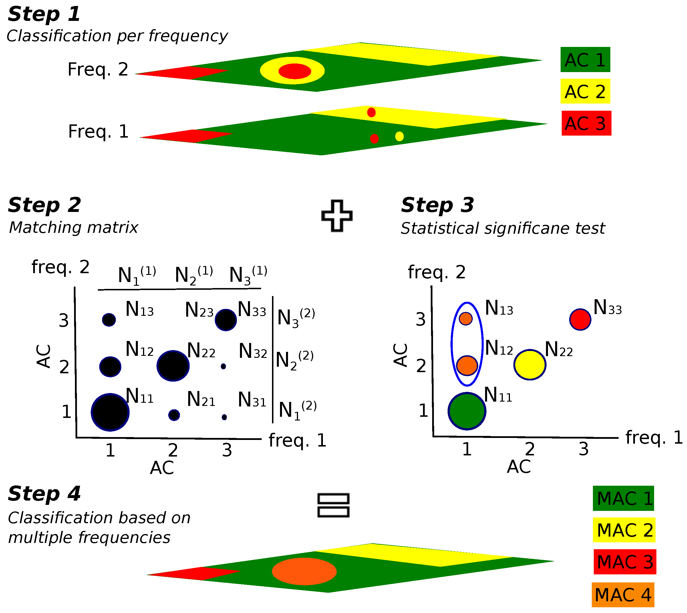
In this study, the decision matrix (Section 3.3) is employed to evaluate the benefit of using additional frequencies for increasing the discrimination performance of the seabed classification method. Each Gaussian distribution obtained from the classification at a single frequency MBES dataset represents a sediment type with specific sediment properties. However, when employing a single frequency, only those sediment types that have a significantly different acoustic response can be distinguished. That means that, if two different sediment types have highly similar acoustic signatures at a specific frequency, they will be represented by the same Gaussian. Considering an additional frequency, the two sediment types may show different acoustic responses and thus can be separated. The question here is whether combining backscatter data, acquired at different frequencies, will actually provide more discrimination possibilities than attainable when using a single frequency only. In order to answer that issue, an approach is needed to establish a single classification map that is derived from the measurements at all frequencies available.
In order to obtain a single classification map from the multispectral data, a four-step algorithm is followed. This is schematically presented in Figure 2, for two frequencies f 1 and f 2 , each having three acoustic classes. The details are described as follows.
Step 1.
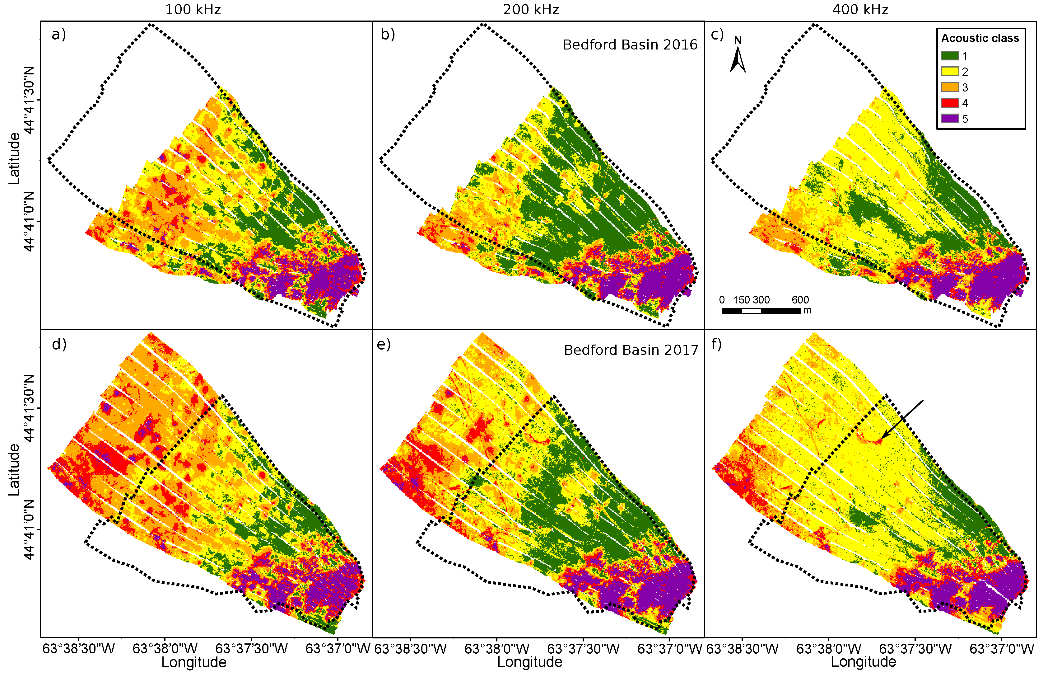
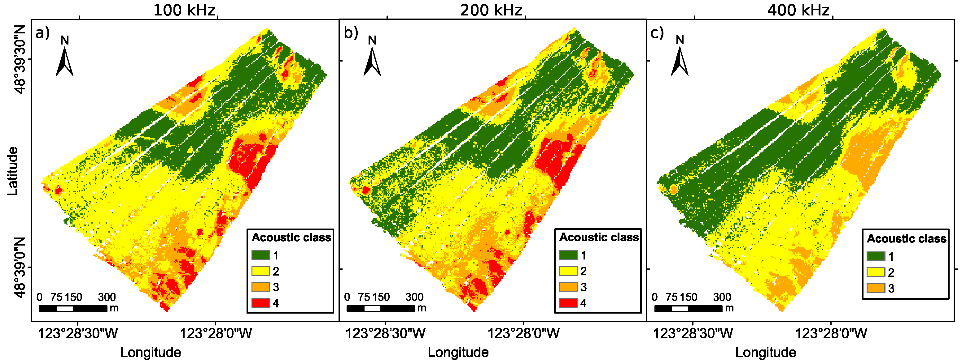
In this step, the Bayesian method is applied to the backscatter histograms per frequency (see Section 3.3). As such, each frequency results in its own classification map (Figure 2).
Step 2.
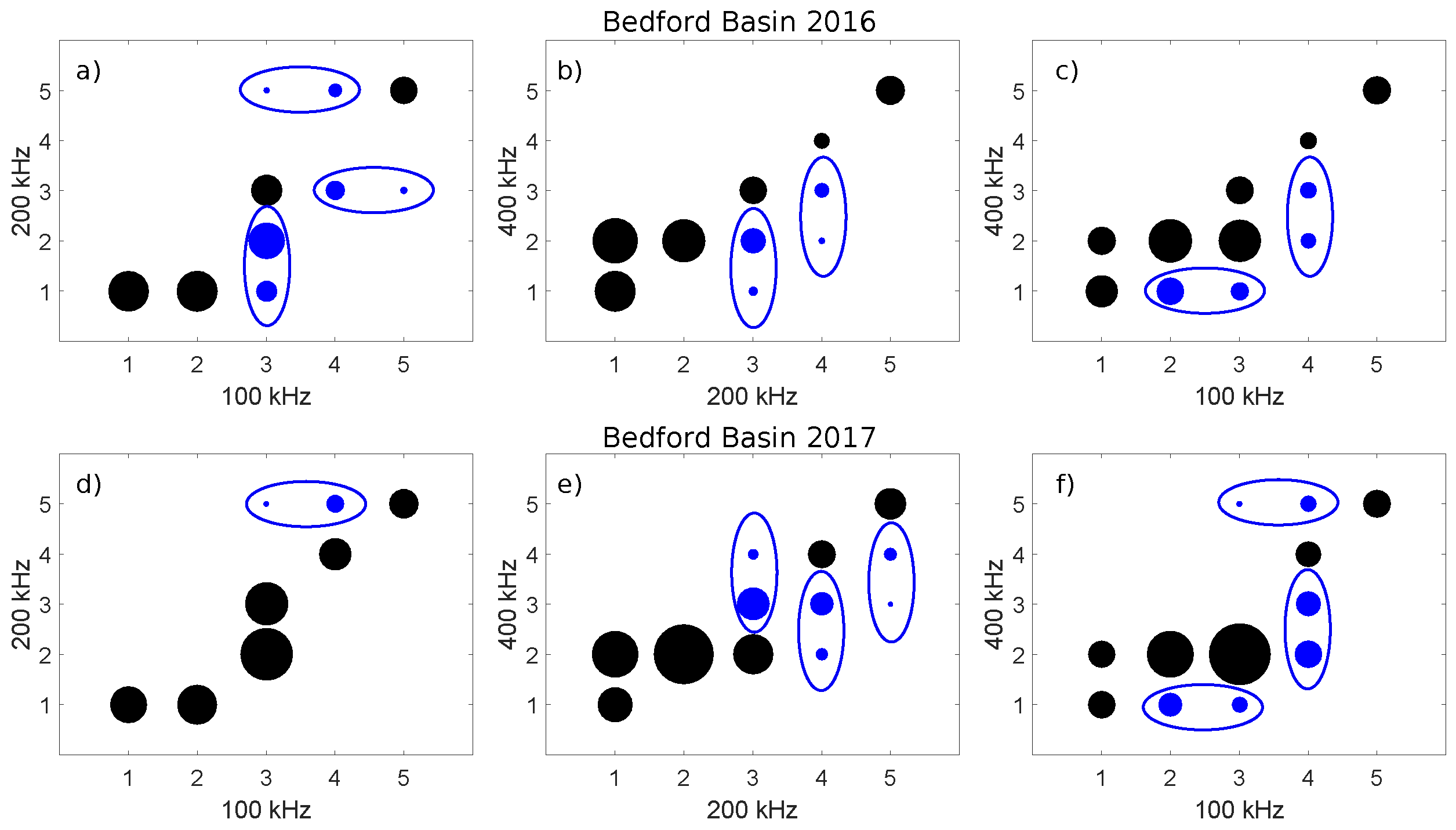
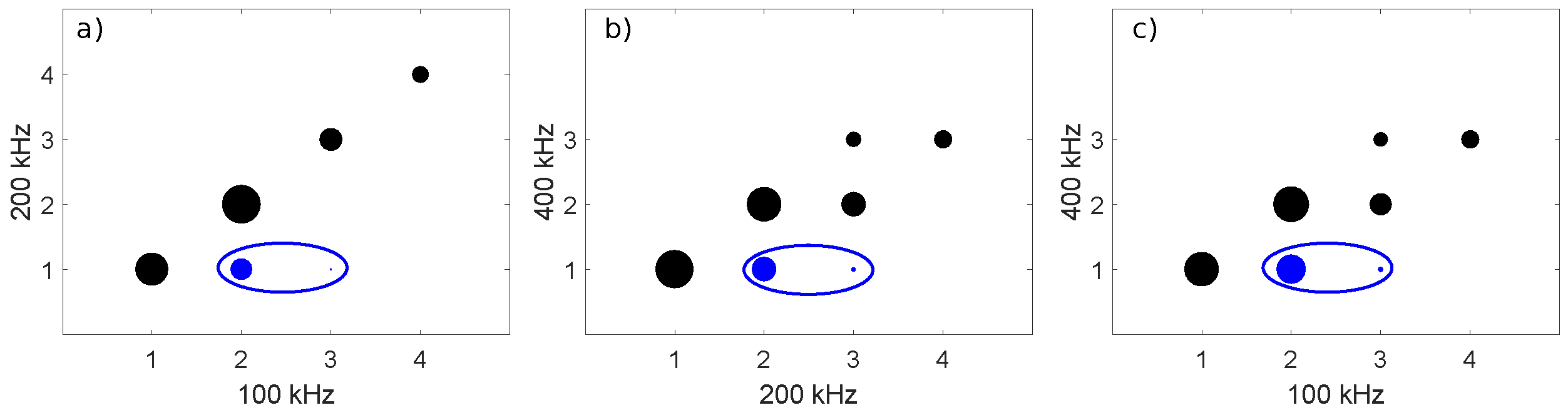
This step calculates the spatial matching between classes obtained from the classification at the individual frequencies (Figure 2). The results are stored in the so-called matching matrix. Each column of the matching matrix represents the locations classified by f 1 , while each row represents the locations classified by f 2 .
Step 3.
The third step is to test whether or not the combinations found are statistically significant. A statistical significance test is performed to assess the actual existence of classes gained by combining the classification results of different frequencies. This statistically corresponds to the null hypothesis H 0 , stated as follows: The AC combination per frequency pair represents an acoustic class. The alternative hypothesis H a is that the AC combination is not statistically significant and due to the occurrence of misclassification. The null hypothesis needs to be tested for every possible acoustic class combination per frequency pair. This is thus performed on all individual elements of the matching matrix (i.e., the nine elements N i , j with i , j = 1 , 2 , 3 , for the example considered in Figure 2).
The statistical significance test is performed by testing the null hypothesis for the combination of AC i and AC j as obtained at f 1 and f 2 , respectively. The null hypothesis is then accepted, if
max N i , j N i ( 1 ) , N i . j N j ( 2 ) > 1 β i , i ( 1 ) β j , j ( 2 )
where N i , j is the number of data points that are simultaneously classified as ACi at f 1 and AC j at f 2 in the entire survey area (see Figure 2). N i ( 1 ) and N j ( 2 ) are the total number of data points classified as ACi at f 1 and ACj at f 2 , respectively. β i , i ( 1 ) is the probability that the class ACi at f 1 is successfully classified (see Equation (11)); β j , j ( 2 ) is accordingly defined for f 2 . A few remarks need to be made:
  • The left-hand side of Equation (12) represents an empirical probability based on the classified real data, whereas the right-hand side expresses a theoretical probability based on the Bayesian decision rule. Therefore, if the empirical probability exceeds the theoretical ones, the null hypothesis is accepted and hence a significant multispectral acoustic class (MAC) is identified. This is in agreement with the statistical significance test, that whenever a variable is larger than its standard deviation, it is considered to be statistically significant.
  • From Equation (12) it follows that, if the occurrence probability of the combination of AC i and AC j , obtained at f 1 and f 2 , is larger than the theoretical probability that this combination occurs due to at least one misclassification (either on f 1 , f 2 or both), then the null hypothesis is accepted. This combination is thus statistically significant and accepted as a MAC. The rejected combinations are supposed not to be statistically significant.
After the testing procedure is applied to the individual entries of the matching matrix, a second testing procedure is started. This concerns only the entries of the matching matrix, which were rejected and hence found not to be significant in the individual tests. This statistically corresponds to make a new null hypothesis H 0 as follows: The AC combination per frequency pair of two neighboring classes represents an acoustic class. The test is applied to the neighboring class combinations. In principle this can be applied to two or more neighboring classes. In this contribution, we limit the approach to two neighboring classes. These two classes can represent statistically significant information and need to be merged as a new acoustic class if the test is accepted. Its probability is derived from the probability set theory according to the identity P ( A B ) = P ( A ) + P ( B ) P ( A B ) , which describes the probability of a union of two sets A and B. The null hypothesis on merging of the two classes gets accepted, if
N i , j + N i , j + 1 N i ( 1 ) > 1 β i , i ( 1 ) β j , j ( 2 ) + β j + 1 , j + 1 ( 2 ) β j , j ( 2 ) β j + 1 , j + 1 ( 2 )
where the probability of a union of two neighboring classes AC j and AC j + 1 at f 2 are derived from the identity P ( A B ) according to β j , j ( 2 ) = P ( A ) , β j + 1 , j + 1 ( 2 ) = P ( B ) and β j , j ( 2 ) β j + 1 , j + 1 ( 2 ) = P ( A B ) . For the data considered in this paper, backscatter measurements are acquired at three frequencies. This means that three sets of frequency pairs need to be considered. This issue is addressed in Step 4.
Step 4.
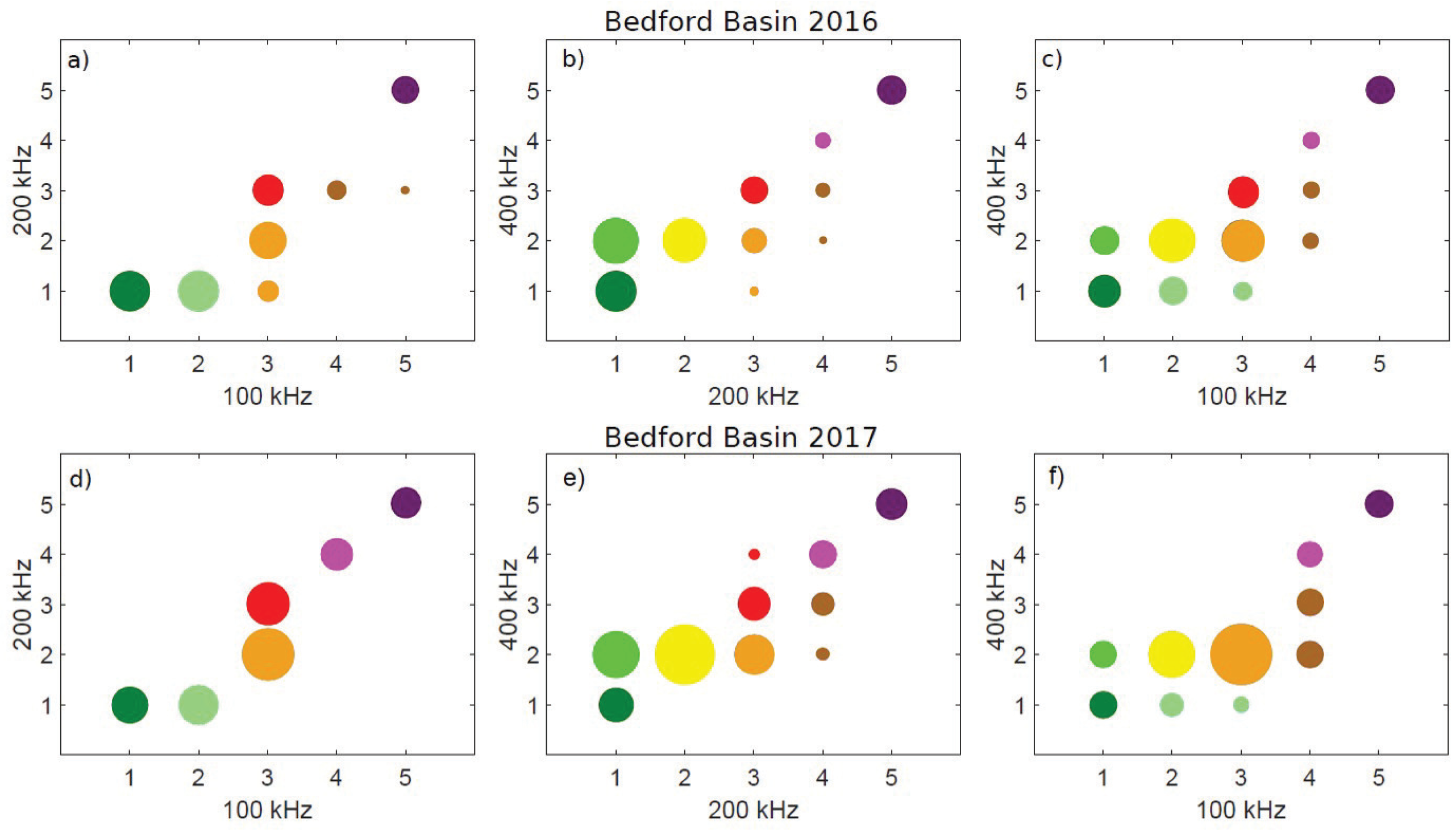
This step generates the acoustic multispectral classification map, i.e., a MAC to each location within the survey area is assigned. In case only two frequencies are employed (as shown in Figure 2), a MAC is assigned to each location according to the corresponding AC combination. Considering n frequencies, the number of frequency pairs increases to k = n ( n 1 ) / 2 , and the generation of the AC map becomes k-dimensional. That means that each location corresponds to k AC combinations. Let us assume that, for each location, we have k numbers of acoustic candidates, i.e., MAC 1 , , MAC k . The most probable candidate is selected to be the final MAC of that location. This is achieved based on the probabilities of the correct classification of frequency pairs. For example, the theoretical probability of the correct classification MAC l of the l th frequency pair is P l = β i , i ( 1 ) l β j , j ( 2 ) l with l = l ( f 1 , f 2 , , f n ) = 1 , , k . Per location, each acoustic candidate has thus a probability of occurrence P l . The acoustic candidate with the highest possible probability is considered to be the most probable one, and hence the corresponding MAC of the frequency pair is obtained. This will be followed to make a unique classification map over available frequency pairs.

4. Results

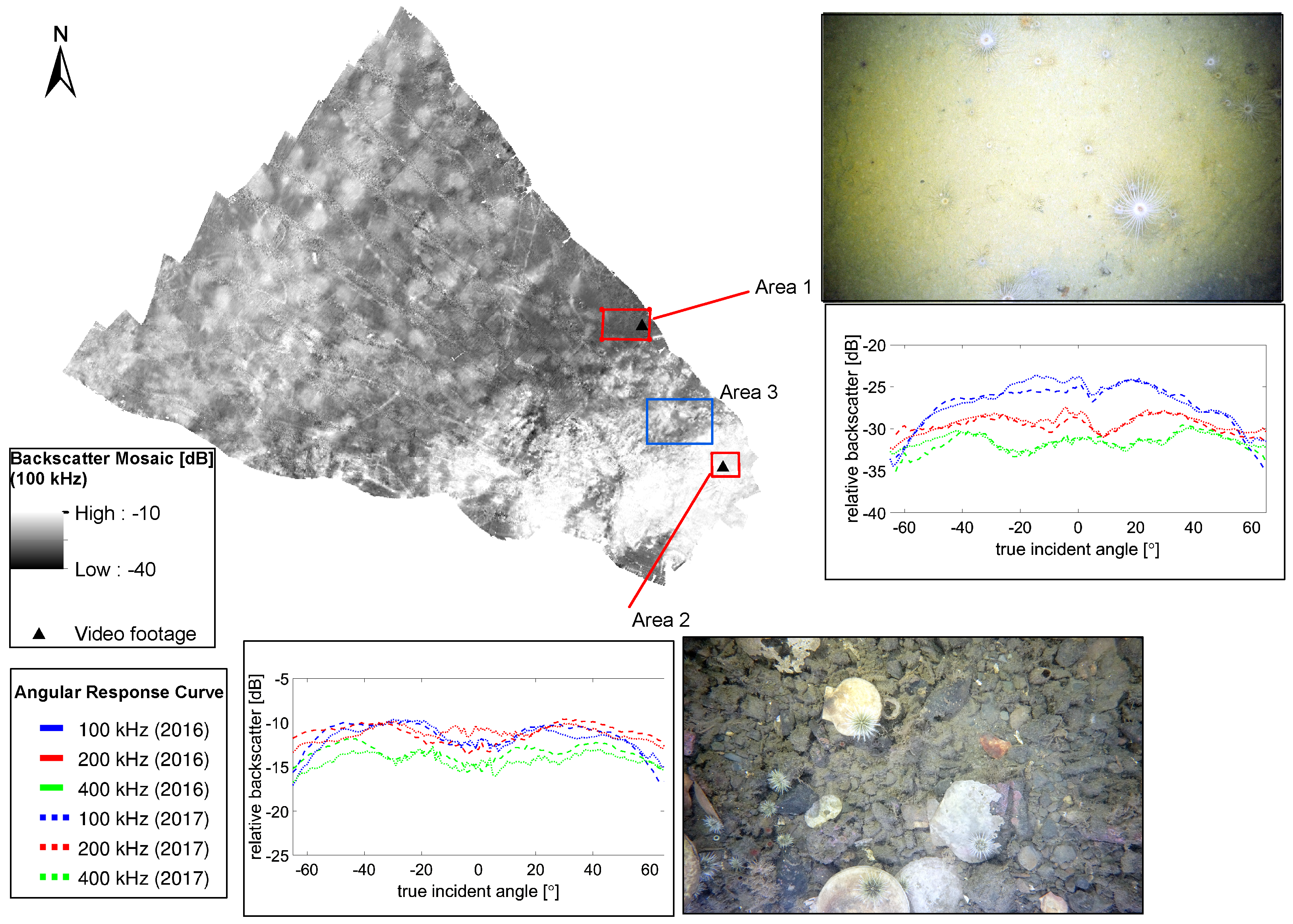
4.1. Verification and Interpretation of Acoustic Data Processing

To investigate the reliability of the acoustic data processing, the angular response curves (ARCs) of the areas that are relatively homogeneous, measured in the Bedford Basin in March 2016 and May 2017, are compared. Here, we assume that the bed characteristics do not change over the considered time and that the same incident angles of both datasets sense the same sediment. To increase the reliability of our assumption, we use data from two different areas of sediments, i.e., a muddy area (Area 1) and a gravel and boulder area (Area 2). The results are displayed in Figure 3. For the majority of the incident angles, the backscatter values of the three frequencies agree with the 2016 and 2017 survey within less than 1 dB. For some incident angles, the deviation reaches up to maximum 2 dB. The backscatter correction appears to be successfully applied considering the good agreement between both datasets.
The shapes of the ARCs corresponding to Area 2 at 200 and 400 kHz are very flat, suggesting a rough seabed with respect to the wavelength. The ARC of 100 kHz is similar except for a significant decrease in the backscatter for incident angles larger than 40 ° , indicating an acoustically smoother seabed. The relatively flat ARC including a missing near-nadir peak can be explained by the APL-UW model [5], where the backscatter strength at 100 kHz for a gravelly area does not have a high variation across the incident angles (Figure 4). In Area 1, the absolute backscatter value is significantly lower compared to Area 2 at each frequency, indicating a softer and smoother seabed, which is confirmed by the video footage showing soft sediments (mud to sand) for Area 1 and a mixture of gravel, boulders, and shells for Area 2. The shape of the ARCs among the different frequencies differ for Area 1. The 100 kHz ARC shows a decrease in backscatter with increasing incident angles as expected from the APL-UW model [5] for fine sediments (Figure 4). The flatness of the ARC shapes increases from 100 to 400 kHz, indicating that the seabed appears acoustically rougher with increasing frequency.
Backscatter mosaics are generated by correcting for the angular dependency using the local Z-score approach with a sliding window of 100 pings and the averaged backscatter value from 30 ° to 60 ° (Figure 5) [37]. No despeckle or anti-aliasing filters are applied to the mosaics to keep the mosaics as unfiltered as possible for the verification of the backscatter processing. The backscatter mosaics indicate a reliable backscatter processing. The backscatter mosaics show clearly different spatial patterns indicating varying sensitivities at the three frequencies for different seabed types. In general, the most pronounced spatial patterns are visible at 100 kHz.

4.2. Application of the Bayesian Method to Multispectral Backscatter Data

4.2.1. Bedford Basin

The Bayesian method is applied to the processed relative backscatter strength per incident angle and frequency. The first step is to average the backscatter values over a range of pings and incident angles (Section 3.3). Accounting for the dependency of the number of scatter pixels per beam, the size of the averaging window in the across-track direction increases from 1.2 ° to 5 ° with a decreasing incident angle and in the along-track direction from 1 to 4 pings with an increasing water depth. In this way, each backscatter value is obtained as the average over a similar number of measurements. In both Bedford Basin datasets, the incident angles greater than 60 ° are found to hold a very low number of backscatter strength values and tend to be noisy. Accounting to these issues, and to receive a robust statistical estimate, the range of incident angles from 40 ° to 60 ° of the starboard and port side are selected as the most suitable and are hence used for estimating the optimal number of acoustic classes per frequency for the 2016 and 2017 Bedford Basin data.
The results are shown in Figure 6a,b where the solid lines and their error bars represent the mean and standard deviation of the reduced- χ 2 values of all considered angles. It is observed that, in general, the averaged reduced- χ 2 values (including the standard deviations) comply with the criterion for an optimal model fit using five Gaussians for all frequencies and for both the 2016 and 2017 datasets. This is indicated by the error bars exceeding the upper dashed line. At 100 kHz for the 2016 dataset, the error bar strikes the upper boundary of the criterion already for four Gaussians, indicating more ambiguous results for that frequency. A further check of the validity of the results is carried out by visually comparing the fit of the modeled Gaussian distributions to the measured histograms. As an example, the fit is displayed for the 54 ° incident angle for the 2016 datasets in Figure 7. Figure 7a–f show increasing improvements with increasing frequency when using five instead of four Gaussians to fit the measured backscatter. These findings are observed for the majority of the considered angles. Based on these results, five classes are selected as optimal for all frequencies. Also visible from Figure 7 is the relatively small number of measurements in each bin, which is caused by the use of the three frequencies subsequently, reducing the measurements per frequency.
According to the requirements for the selection of the reference angles, stated in Section 3.3, incident angles of 53 ° , 54 ° , and 55 ° for the 2016 dataset and 45 ° , 47 ° and 49 ° for the 2017 dataset are chosen. For the generation of the final AC maps, the incident angles from 10 ° to 60 ° for the 2016 datasets and from 10 ° to 64 ° for the 2017 datasets are considered. The backscatter data around nadir are prone to specular reflection and are therefore too noisy to provide a reliable classification. The final AC maps for 100, 200, and 400 kHz are displayed in Figure 8.
The single-frequency AC maps obtained from the 2016 and 2017 datasets largely agree for the overlapping area. A crescent-shaped feature visible in the north of the 200 and 400 kHz maps ( AC 3 and AC 4 , indicated by the arrow in Figure 8f) of the 2017 datasets, is not present in the 2016 AC maps, indicating a change in the seabed over time. This feature is also not present in the 2016 backscatter mosaics (Figure 5). In addition, the central area in the 400 kHz map is more extensively covered with AC 1 in the 2016 map than in the 2017 map. Natural phenomena, e.g., the deposition of finer sediments, might have changed the seabed properties over time. However, the difference is only about one acoustic class. In general, the comparison of the 2016 and 2017 maps indicates the robustness of the classification method applied to each frequency separately.
Four main differences between the different frequencies are observed. First, in the northern part of the survey area, acoustic classes are higher for the low frequencies ( AC 3 and AC 4 for 100 and 200 kHz) than for the highest frequency ( AC 1 and AC 2 for 400 kHz). Second, the spatial patterns are different, in particular between 100 and 400 kHz. In Figure 8a,d and partly in Figure 8b,e, circular features are visible in the central part and classified as AC 3 and AC 4 in 100 and partly in 200 kHz. In the 400 kHz map, these features are not apparent and the locations are classified as AC 2 or AC 1 , like the surrounding seabed. Third, a straight orange line ( AC 3 ) from NNW-SSE is clearly visible at 400 kHz, less pronounced at 200 kHz, and absent at 100 kHz. A fourth noticeable difference is the spatial distribution of AC 2 and AC 1 . AC 2 (yellow) covers a large area in the central part of the 400 kHz map compared to a very limited extent of AC 2 and a larger extent of AC 1 in the 100 and 200 kHz map. This indicates that AC 1 and AC 2 of 100 and 200 kHz represent different seabed properties than AC 1 and AC 2 of 400 kHz. The south-east part of the study area shows the same spatial structures between the frequencies and the datasets from 2016 and 2017. In particular, AC 5 represents this part of the seabed. It demonstrates that this part of the seabed has the same acoustic response per frequency, and no additional information can be gained by using multi-frequency data. In general, the most visible differences are between the AC maps obtained at 100 and 400 kHz.

4.2.2. Patricia Bay

For the measurements taken in Patricia Bay, an optimal fit to the measured histograms of 100 and 200 kHz can be achieved by using four Gaussians—that of 400 kHz using three Gaussians (Figure 6c). The determination of the AC boundaries is based on the incident angles of 54 ° , 55 ° , and 56 ° . These angular ranges provide the most consistent results for the Patricia Bay datasets. The AC maps per frequency are displayed in Figure 9. The spatial patterns are very consistent over the different frequencies, unlike the Bedford Basin. The main difference is that the area being classified as AC 3 at 400 kHz is subdivided into two classes ( AC 3 and AC 4 ) at 100 and 200 kHz. In that regard, the lower frequencies have a higher discrimination for that part of the seabed.
Comparing the Patricia Bay and Bedford Basin, the results indicate (1) more ACs can be distinguished in the Bedford Basin and (2) the sensitivity per frequency to the seabed properties differs at the two study sites. The first is expected to be directly related to the variety in sediments in the two areas. The latter indicates that the discrimination potential per frequency is highly dependent on the sensed seabed, so the selection of the ideal frequency or frequency combinations depends on the considered study site.

4.3. Evaluation of the Benefit of Using Multiple Frequencies

4.3.1. Bedford Basin

The matching matrix, obtained from Step 2, has entries for almost all AC combinations for each of the frequency pairs (not shown here). The statistically significant AC combinations per frequency pair, identified in Step 3, are visualized in Figure 10. The black circles indicate the resulting AC combinations, where each AC per frequency is considered individually (the first part of Step 3) and the blue circles represent AC combinations where neighboring classes of one frequency are considered together (the second part of Step 3). The 2016 and 2017 data show very similar patterns. A few exceptions exist and can be related to the larger acquisition area in 2017. For example, the combination of AC 3 and AC 3 between 100 and 400 kHz is classified as statistically significant in 2016, whereas it is insignificant in 2017. Figure 10 demonstrates that the combination of 100 and 200 kHz exhibits the lowest number of remaining AC combinations for both the 2016 and 2017 dataset. Seven combinations are present (including pairs of blue circles which are counting as one class), i.e., two additional classes are revealed by the multispectral measurement. In the 2017 dataset, the combinations of 200–400 and 100–400 kHz have the same amount of remaining combinations even though they are slightly different. In the 2016 dataset, 100 and 400 kHz have the most remaining AC combinations, indicating that most of the information on the seabed in this study area can be retrieved from combining 100 and 400 kHz.

4.3.2. Patricia Bay

For Patricia Bay, the combinations of the 100–400 and 200–400 kHz backscatter datasets reveal the most additional information (six remaining AC combinations) about the seabed (Figure 11). However, the number of remaining AC combinations is significantly lower compared to the Bedford Basin.

4.4. Combination of Multiple Frequencies

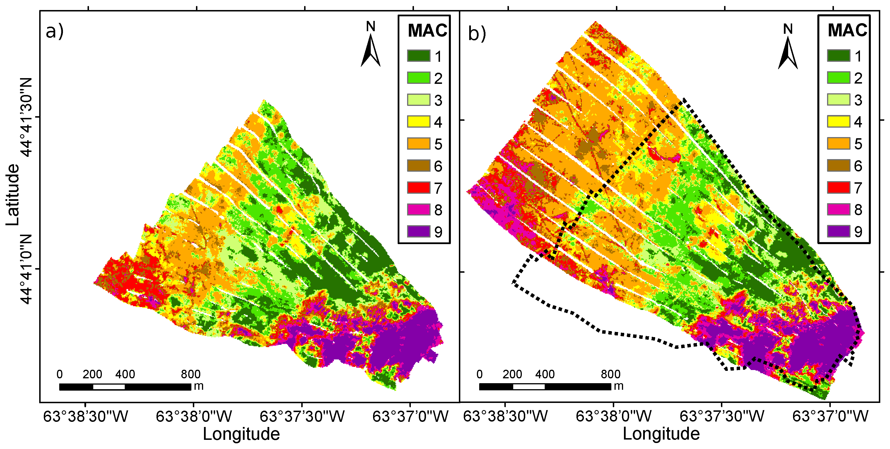
4.4.1. Bedford Basin

In this section, the information provided per frequency is combined with the aim to generate a multispectral classification map. The MACs are defined from the statistically significant AC combinations per frequency pair. Figure 10 shows that this yields 10 and 11 unique MACs considering all frequency pairs for the 2016 and 2017 datasets, respectively. Here, we employ three frequency pairs (100–200, 200–400, and 100–400 kHz), which means that each grid cell corresponds to three AC combinations. The application of Step 4 identifies the most probable AC combinations out of the three possible combinations. It is observed that one and two MACs for the 2016 and 2017 datasets, respectively, have low probabilities compared to the other classes and less than 2% of the grid cells are assigned to these classes. In addition, their distribution within the study area is very scattered, so they are considered to be insignificant yielding to a reduction to nine MACs for both datasets (see Figure 12).
The final multispectral maps are shown in Figure 13. The different spatial patterns observed in each of the single-frequency acoustic classification maps (100, 200, and 400 kHz) are now all visible in the combined map. The circular features, mainly visible in the 100 kHz map and less pronounced in the 200 kHz map, are clearly visible in the combined map ( MAC 5 and MAC 6 ). In addition, they are now distinguishable from the structure in the north-west of the study area. Moreover, the SW-NE stripes (according to [18], these features represent trawl marks) are clearly distinguished in the final map from the surrounding seabed in the 2017 dataset. This feature is only clearly visible in the 400 kHz in 2017 and slightly in the 200 kHz map, but does not show up in the 100 kHz map. The softer sediments (lower AC and lower backscatter) show a higher discrimination in the final MAC map. AC 1 of 100 kHz (dark green in Figure 8a) and AC 1 and AC 2 of 200 and 400 kHz (dark green and yellow in Figure 8b,c) are converted to three separated MACs in the final map, indicating a reliable geological spatial pattern. Overall there is a good agreement between the overlapping area of the 2016 and 2017 multispectral map. Assuming the seabed remained unchanged over this period of time, this observation shows the robustness of the classification approach. In general, the higher MACs seem to be more persistent over time than the lower MACs, which indicates that sediments correlating to the higher MACs (probably harder and rougher sediments) are either
  • more temporarily and spatially stable or
  • acoustically less affected to slight changes in the sediment composition; for example, deposition of small amount of sand on a muddy sediment affects the resulting backscatter more than that on gravelly sediment does.
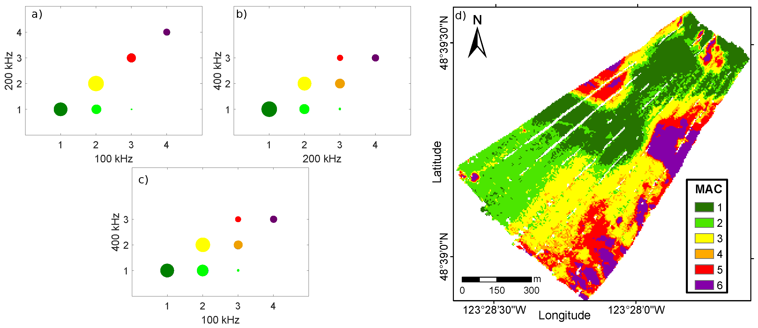
A detailed spatial and temporal ground-truth sampling effort is needed to indicate the contributions of the above-mentioned issues.

4.4.2. Patricia Bay

The multispectral backscatter data of the Patricia Bay reveal six classes (Figure 14a–c). All of these classes are already present using 200 and 400 kHz or 100 and 400 kHz (Figure 14b,c). This indicates that the use of 100 or 200 kHz together with 400 kHz is sufficient to gather all acoustic information from the seabed.
The multispectral map of the Patricia Bay is shown in Figure 14d. The areas represented by MAC 4 to MAC 6 do not show a significant higher discrimination compared to the single-frequency map of 100 and 200 kHz. AC 1 and AC 2 are represented in the multispectral map as MAC 1 , MAC 2 , and MAC 3 , which indicates an improved discrimination. However, the improved acoustic discrimination due to the use of multi-frequency backscatter is higher for the Bedford Basin.

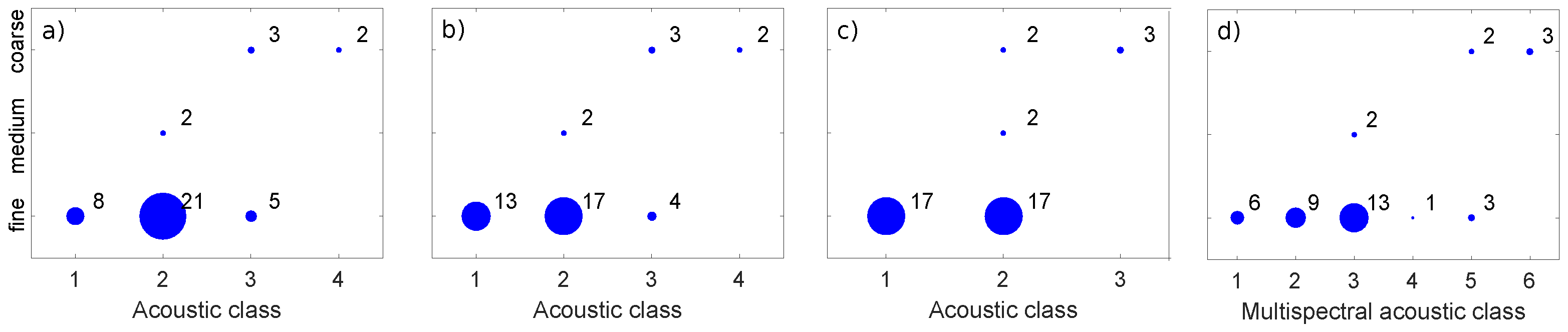
4.5. Correspondence between Ground-Truth and Acoustic Classification

In this section, the acoustic classification results are quantitatively compared with the ground-truth data. For this, the mode (most frequently occurring value) of the acoustic classes within a radius of 10 m around the geographical location of the ground-truth data are calculated.

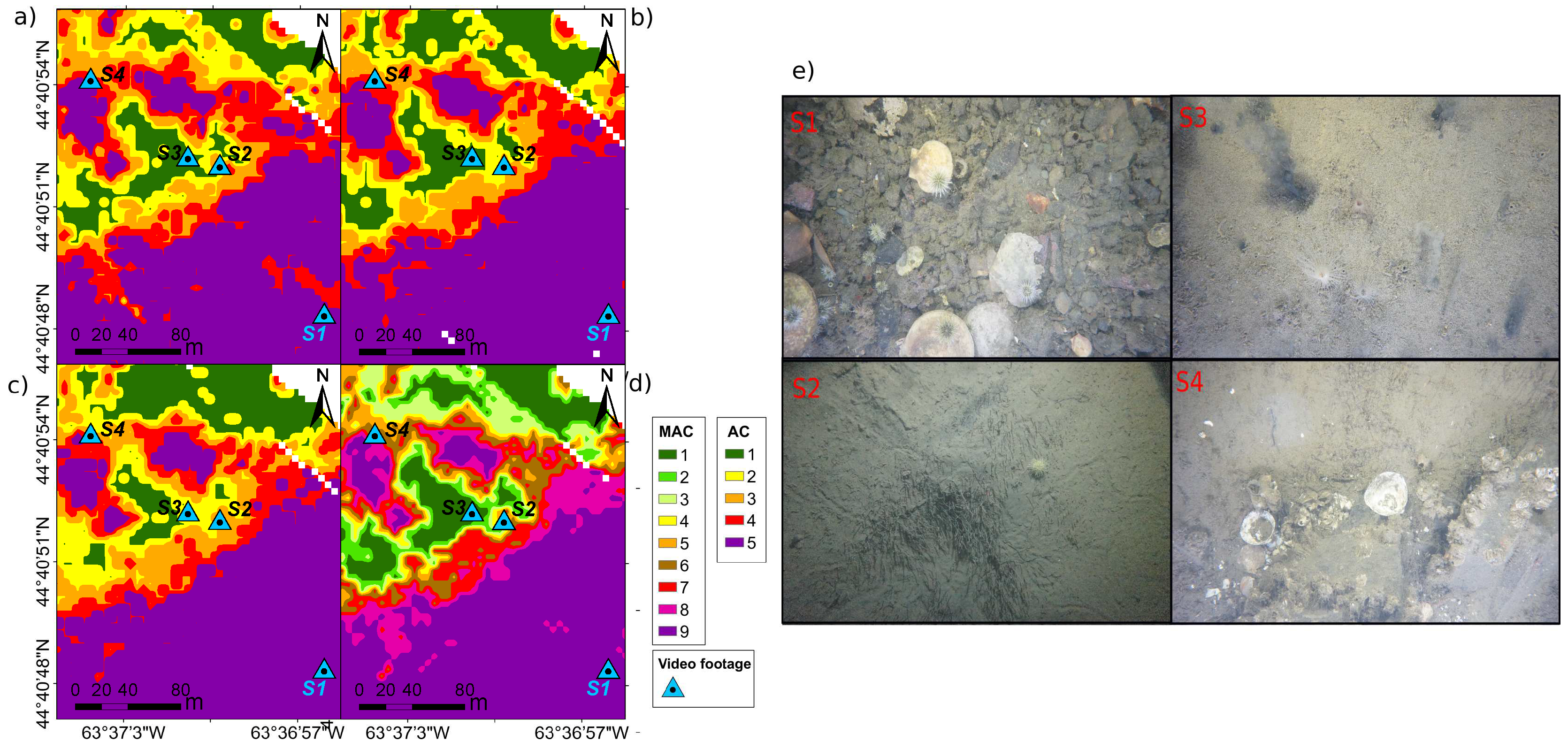
4.5.1. Bedford Basin

Figure 15 shows, for all locations where video data are available, the acoustic class and the classification based on the video data. It is seen that each frequency shows that AC 1 and AC 2 typically correspond to the soft sediment class, whereas the highest AC matches with the hard substrate. AC 1 and AC 2 indicate that, acoustically, a more detailed discrimination of the fine sediments can be made compared to that based on the video data. AC 3 indicates the presence of a soft substrate but also occurs in the mixed category. The mixed category spreads along AC 3 to AC 5 for all frequencies. These samples are located at the transition between hard to soft sediments and are part of a heterogeneous environment (an example is given in Figure 16). A certain inaccuracy of the geographical location of the video footage or that the video footage represents only a small part of the seabed (ca. 40 cm × 40 cm) may cause the spread. The hard substrate is represented solely by AC 5 . The multispectral results show a similar correspondence. As with the single-frequency results, this indicates a higher capability to discriminate sediment classes based on acoustics compared to that based on the video data. Combining the frequencies increases this performance even further. Here it should be noted that the different frequencies might sense different depths depending on the sediments. This aspect will be further addressed in Section 5. The high MACs again indicate the hard and mixed sediment classes to the same extent as the single-frequency results.
More detailed and qualitative classification results and video footage samples are shown in Figure 16. Clearly, the highest AC and MAC represent a seabed extensively covered with boulders, shells, and gravel, as indicated by Video Footage Sample S1 (sample means here the location of the video footage). Sample S4 displays a mixture of boulders, gravel, and coral reef with soft sediments. In all maps, this sample is located at the boundary between the higher and lower ACs and MACs, indicating the transition area from hard to soft substrates. Samples S2 and S3 are assigned to the soft sediment category, but a more detailed observation indicates differences in the seabed composition: S2 consists of a soft sediment slightly covered with benthic flora, whereas S3 consists of soft sediment combined with some benthic flora as well as benthic fauna and gas seeps. In the three single-frequency classification maps as well as in the multispectral classification map, Samples S2 and S3 are acoustically separated.

4.5.2. Patricia Bay

The acoustic classes are shown together with the ground-truth data (grab samples) categorized into fine, medium, and coarse for the Patricia Bay in Figure 17. Each frequency shows that AC 1 solely corresponds to the fine sediment class and that the highest AC indicates the coarse substrate.
The majority of AC 2 corresponds to the fine sediment class (21, 17, and 17 samples for 100, 200, and 400 kHz) as well, whereas two samples also correspond to the medium sediment class. At 400 kHz, AC 2 corresponds also to the coarse sediment class. AC 3 corresponds to the fine and coarse sediment class at 100 and 200 kHz, indicating a very ambiguous result. The multispectral classes indicate a higher capability of multispectral backscatter to discriminate between the fine sediment classes compared to the single frequency classification. However, the MAC shows a similar performance for the medium and hard class as the ACs, which indicates no increased discrimination.

5. Discussion

We have proposed a classification algorithm capable of classifying multispectral backscatter by combining the information obtained at different frequencies into a single classification map. The utilization of the multispectral backscatter data from three different MBES datasets (Bedford Basin 2016, Bedford Basin 2017 and Patricia Bay 2016) reveals three main findings.
(1)
Combining 100 and 400 kHz, in general, reveals the most additional information about the seabed. This is in agreement with the study of Hughes Clark [17], who pointed out that at least a frequency spacing of one octave is required to use the frequency dependency of backscatter but that a separation of two octaves (100 vs. 400 kHz ) is desired.
(2)
The use of multiple frequencies allows for a better acoustic discrimination of seabed sediments than single-frequency data. For all datasets, in particular for the Bedford Basin, more MACs are revealed than ACs by applying the multispectral classification algorithm. However, careful interpretation of the additional classes is required. There are three possible reasons: (i) the relationship between roughness and acoustic wavelength, (ii) a dominating scattering regime, and (iii) signal penetration. The first and second issue reflect the additional discrimination of the surficial sediments, whereas the third reason combines information from different depths at the seabed. Insights into the relative importance of the above factors are needed to interpret the MAC map.
(3)
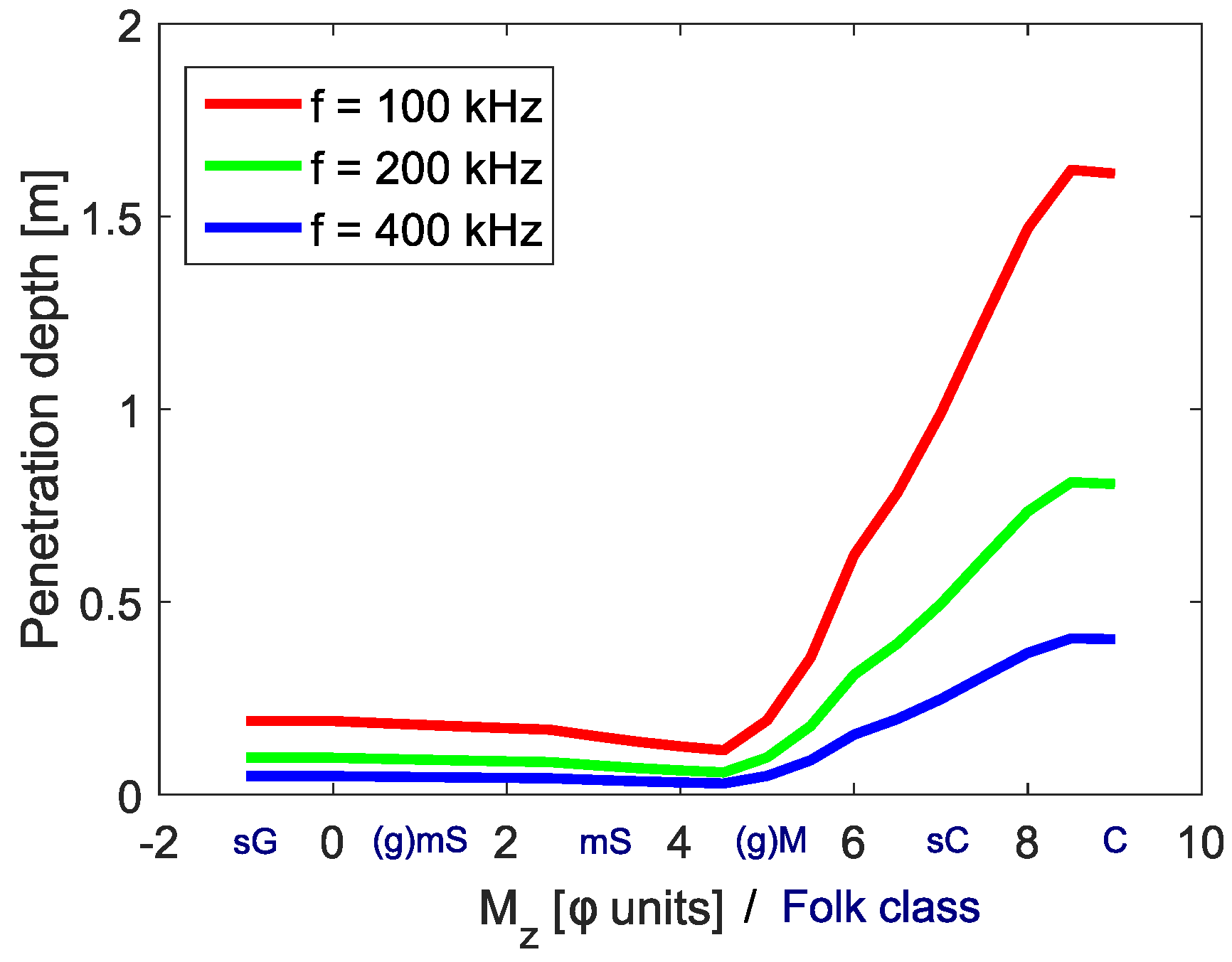
The optimal frequency selection for ASC depends on the local seabed. The results from two different study areas have shown that the most discriminative frequency and the benefit of using multiple frequencies for ASC highly depends on the local seabed, and a general conclusion cannot be drawn. In the Bedford Basin, a significantly increased discrimination performance is observed, which seems to be mainly based on the increasing signal penetration from 400 to 100 kHz. In Patricia Bay, we observed only a slightly increased discrimination performance. This might result from the fact that the finest sediment in that area is muddy sand and the corresponding signal penetration does not differ very much for the different frequencies. However, we need to consider that the 10-year time difference between ground truthing and acoustic data acquisition results in unknown uncertainties. The surficial sediment distribution might have changed within this period.
For the results presented here, mostly an increased discrimination (more classes) using multiple frequencies is found for the finer sediments. For these sediment types, it is known that the signal penetration for 100 kHz is higher than for 400 kHz. Figure 18 indicates the larger signal penetration of the lower frequencies for fine sediments. The transition from sand to mud (Mz = 4.5 φ ) approximately determines the point where the signal penetration of 100 and 400 kHz diverges. This indicates that at least to some extent additional classes are caused by combining information from the surface sediments (400 kHz) with information from the shallow subsurface (100 kHz). These findings are supported by Brown et al. [18], who employed the same multispectral backscatter dataset acquired in 2016 in the Bedford Basin. They concluded that depending on the thickness of the fine sediment layer (mud), the backscatter at 100 kHz results from rough dredge spoils buried in the shallow subsurface below the fine sediments. In contrary, the backscatter at 400 kHz reflects only the surface sediments due to the limited signal penetration.
Coarse sediments are expected to show similar signal penetration depths for the three frequencies (Figure 18). Therefore, it can be expected that the backscatter at different frequencies reflects mostly the surface sediments, and a possible frequency dependency of the backscatter is caused by a change in the dominating scattering regime and the relationship between roughness and acoustic wavelength. However, in this study, the coarser sediments (boulder/gravel) are represented consistently by the highest AC at each frequency (see Figure 8), indicating a limited frequency dependency for the considered coarser sediments. Similar findings for coarser sediments were found by Brown et al. [18] for the same study area and in [13,17] for different study areas.
Further research is needed to investigate to what degree the frequency dependency contributes to an improved acoustic discrimination by either the relationship between roughness and acoustic wavelength or the dominating scattering regime on the backscatter. Regarding the latter, the use of multispectral backscatter is promising to solve the ambiguous relationship between backscatter and sediments, where the mean grain size of the sediments is roughly equal to the acoustic wavelength. This ambiguity was observed in several studies and might correspond to the change in the scattering regime from Rayleigh to geometrical scattering [7,8,15,16,39]. The ambiguity occurs, in particular, for coarser sediments (gravelly sand to gravel), where the mean grain size ranges around the acoustic wavelength (for a frequency of 300 kHz). Therefore, the use of frequencies ranging from 100 to 400 kHz might result in an increased discrimination performance of the coarser sediment types.

Benefits Versus Drawbacks of Multispectral Backscatter

The study has shown that the acoustic maps of the different frequencies do not necessarily represent exactly the same part of the seabed with respect to depth. This can support interpretation of the backscatter or classification maps, for example, in cases where a discrepancy between the acoustic classification and other measurement exist, such as surficial seabed samples (e.g., Van Veen samples) indicating a fine sediment and acoustic measurements (e.g., 100 kHz) indicating high backscatter strength. In such a case, the availability of a higher frequency (e.g., 400 kHz) adds crucial information to interpret this issue in terms of depth and to investigate whether the backscatter results from coarser sediments below the fine sediment layer. However, further research studies (e.g., using shallow cores) are needed to investigate to what extent different depths of the seabed contribute to the total backscatter strength to ultimately assign depth values to the MACs.
The acquisition of multispectral backscatter is, in general, possible without any loss of time compared to the acquisition of monochromatic backscatter. This is due to the ability of the R2Sonic 2026, which transmits multiple frequencies on a ping-by-ping basis. However, we need to consider that some disadvantages coming along with this approach: (1) the survey depth is limited to the highest frequency caused by the increased signal attenuation in the water column, (2) data coverage in the along-track direction is reduced with increasing number of considered frequencies, and (3) the spatial resolution of the bathymetry is restricted by the beam footprint of the lowest frequency. That means that a trade-off between benefits and disadvantages exists and that the use of the multispectral mode of such an MBES highly depends on the aim of the survey and the seabed characteristics in the survey area.

6. Conclusions

In this paper, the Bayesian acoustic sediment classification (ASC) method is introduced for the classification of multispectral MBES backscatter. The method accounts for the natural variability of the backscatter strength by assuming the measured backscatter per beam and frequency to result in a number of discrete seafloor types that each corresponds to a Gaussian distribution. In that regard, the acoustic classes (ACs) are defined per frequency and incident angle, which allows for an evaluation and comparison among the ACs obtained at different frequencies. We developed a classification algorithm where the classification results obtained from the different frequencies are combined to a so-called multispectral acoustic class map.
The multispectral Bayesian method is applied to a multi-frequency (100, 200 and 400 kHz) backscatter dataset acquired with an R2Sonic 2026 MBES in the Bedford Basin, Canada, in 2016 and 2017 and in the Patricia Bay, Canada, in 2016. The system allows for the use of different operating frequencies on a ping-by-ping basis. The performed data processing accounts for most sonar settings and environmental conditions affecting the backscatter strength at different frequencies. It is shown that the multispectral backscatter can be properly processed to be used for ASC.
The main results are threefold: (1) combining 100 and 400 kHz, in general, reveals the most additional information about the seabed; (2) the use of multiple frequencies allows for a larger acoustic discrimination than based on a single frequency; and (3) the optimal frequency selection for ASC depends on the local seabed.
The comparison of the multispectral acoustic class maps obtained from the Bedford Basin acquired in 2016 and 2017 shows high agreement. Assuming temporarily constant seabed properties, this indicates the robustness of the introduced multispectral classification method. The applicability of this method to multispectral backscatter is further shown by the successful application to a dataset acquired in a very different marine environment (Patricia Bay). The produced maps combine the acoustic information obtained at monochromatic backscatter into a single map, thereby providing an overview of acoustical different areas, which can be used for future ground truthing campaigns. However, this map combines information from both the seabed and the shallow subsurface due to an increased signal penetration for the lower frequencies and finer sediments. Considering the used frequency range from 100 to 400 kHz, it is in particular the case for muddy sediments (Bedford Basin).
At this time, a quantification of the gained benefit from different acoustic frequencies using the existing video footage cannot clearly be accomplished for both study areas. Additional video footage and physical samples from the seabed and subsurface would be required at predefined locations. Still, a qualitative comparison to the video footage and a geological interpretation of the Bedford Basins indicates an improved discrimination by combining 100, 200, and 400 kHz to a multispectral acoustic class map.
The research of multispectral MBES backscatter is just in its initial implementation stage. The acoustic response of different sediment types for different frequencies has to be studied in more detail, which requires extensive ground truthing. It has to be investigated to what extent the backscatter signal contains contribution from both the seabed and the shallow subsurface. Finally, the establishment of reference areas for MBES backscatter calibration will provide promising opportunities to calibrate and secure an appropriate processing of multispectral backscatter.

Author Contributions

Conceptualization, T.C.G., T.A.T.A., M.S., and D.G.S.; Data curation: T.C.G.; formal analysis, T.C.G. and A.A.-S.; Methodology, T.C.G., M.S., A.A.-S., and D.G.S.; software, T.C.G.; validation, T.C.G. and A.A.-S.; writing–original draft preparation, T.C.G. and T.A.T.A.; writing—review and editing, T.C.G., M.S., A.A.-S., T.A.G.P.v.D., and D.G.S.; visualization, T.C.G. and T.A.T.A.; supervision, M.S., T.A.G.P.v.D., and D.G.S.; funding acquisition, M.S., D.G.S., and T.A.G.P.v.D.

Funding

This investigation is part of a Ph.D. research, funded by Royal Boskalis Westminster N.V., a dredging and marine installations company, and the research institute Deltares, Netherlands, for applied research in the fields of water and the subsurface.

Acknowledgments

The authors would like to thank R2Sonic for providing the multispectral multibeam datasets of the Bedford Basin (2016 and 2017) and Patricia Bay (2016), and for their very helpful discussions regarding software and hardware implementations. Further, many thanks go to the group of Prof. Jens Greinert from the Geomar–Helmholtz Centre for Ocean Research Kiel for giving us access to their software tool to read the sonar data files.

Conflicts of Interest

The authors declare no conflict of interest.

References

  1. Lecours, V.; Dolan, M.F.J.; Micallef, A.; Lucieer, V.L. A review of marine geomorphometry, the quantitative study of the seafloor. Hydrol. Earth Syst. Sci. 2016, 20, 3207–3244. [Google Scholar] [CrossRef] [Green Version]
  2. Brown, C.J.; Smith, S.J.; Lawton, P.; Anderson, J.T. Benthic habitat mapping: A review of progress towards improved understanding of the spatial ecology of the seafloor using acoustic techniques. Estuar. Coast. Shelf Sci. 2011, 92, 502–520. [Google Scholar] [CrossRef]
  3. Jackson, D.R.; Richardson, M.D. High-Frequency Seafloor Acoustics. In High-Frequency Seafloor Acoustics; Springer: New York, NY, USA, 2007. [Google Scholar] [CrossRef]
  4. Williams, K.L.; Jackson, D.A.; Tang, D.; Briggs, K.B.; Thorsos, E.I. Acoustic Backscattering from a Sand and a Sand/Mud Environment: Experiments and Data/Model Comparisons. IEEE J. Ocean. Eng. 2009, 34, 388–398. [Google Scholar] [CrossRef]
  5. Applied Physics Laboratory, University of Washington. APL-UW High-Frequency Ocean Environmental Acoustic Models Handbook; Technical Report APL-UW TR9407; Applied Physics Laboratory, University of Washington: Seattle, WA, USA, 1994. [Google Scholar]
  6. Medwin, H.; Clay, C. Fundamentals of Acoustical Oceanography; Elsevier Inc.: Amsterdam, The Netherlands, 1998. [Google Scholar] [CrossRef]
  7. Ivakin, A.N.; Sessarego, J. High frequency broad band scattering from water-saturated granular sediments: Scaling effects. J. Acoust. Soc. Am. 2007, 122, 165–171. [Google Scholar] [CrossRef] [PubMed]
  8. Buscombe, D.; Grams, P.E.; Kaplinski, M.A. Compositional Signatures in Acoustic Backscatter over Vegetated and Unvegetated Mixed Sand-Gravel Riverbeds. J. Geophys. Res. Earth Surf. 2017, 122, 1771–1793. [Google Scholar] [CrossRef]
  9. Ryan, W.B.F.; Flood, R.D. Side-looking sonar backscatter response at dual frequencies. Mar. Geophys. Res. 1996, 18, 689–705. [Google Scholar] [CrossRef]
  10. Guillon, L.; Lurton, X. Backscattering from buried sediment layers: The equivalent input backscattering strength model. J. Acoust. Soc. Am. 2001, 109, 122–132. [Google Scholar] [CrossRef]
  11. Schneider von Deimling, J.; Weinrebe, W.; Tóth, Z.; Fossing, H.; Endler, R.; Rehder, G.; Spieß, V. A low frequency multibeam assessment: Spatial mapping of shallow gas by enhanced penetration and angular response anomaly. Mar. Pet. Geol. 2013, 44, 217–222. [Google Scholar] [CrossRef] [Green Version]
  12. Jackson, D.R.; Baird, A.M.; Crisp, J.J.; Thomson, P.A.G. High-frequency bottom backscatter measurements in shallow water. J. Acoust. Soc. Am. 1986, 80, 1188–1199. [Google Scholar] [CrossRef]
  13. Urick, R.J. The backscattering of Sound from a Harbor Bottom. J. Acoust. Soc. Am. 1954, 26, 231–235. [Google Scholar] [CrossRef]
  14. Hefner, B.T.; Jackson, D.R.; Ivakin, A.M.; Tang, D. High frequency measurements of backscatttering from heterogeneities and discrete scatteres in sand sediments. In Proceedings of the Tenth European Conference on Underwater Acoustics (ECUA2010), Istanbul, Turkey, 5–9 July 2010; Volume 3, pp. 1386–1390. [Google Scholar]
  15. Eleftherakis, D.; Snellen, M.; Amiri-Simkooei, A.R.; Simons, D.G. Observations regarding coarse sediment classification based on multi-beam echo-sounder’s backscatter strength and depth residuals in Dutch rivers. J. Acoust. Soc. Am. 2004, 135, 3305–3315. [Google Scholar] [CrossRef] [PubMed]
  16. Snellen, M.; Gaida, T.C.; Koop, L.; Alevizos, E.; Simons, D.G. Performance of multibeam echosounder backscatter-based classification for monitoring sediment distributions using multitemporal large-scale ocean data sets. IEEE J. Ocean. Eng. 2018, 99, 1–14. [Google Scholar] [CrossRef]
  17. Hughes Clark, J.E. Multispectral Acosutic Backscatter from Multibeam, Improved Classification Potential. In Proceedings of the United States Hydrographic Conference, National Harbor, MD, USA, 15–19 March 2015. [Google Scholar]
  18. Brown, C.J.; Beaudoin, J.; Brissette, M.; Gazzola, V. Setting the Stage for Multispectral Acoustic Backscatter Research. In Proceedings of the United States Hydrographic Conference, Galveston, TX, USA, 20 March 2017. [Google Scholar]
  19. Lu, D.; Weng, Q. A survey of image classification methods and techniques for improving classification performance. Int. J. Remote Sens. 2007, 28, 823–870. [Google Scholar] [CrossRef] [Green Version]
  20. Simons, D.G.; Snellen, M. A Bayesian approach to seafloor classification using multi-beam echo-sounder backscatter data. Appl. Acoust. 2009, 70, 1258–1268. [Google Scholar] [CrossRef]
  21. Alevizos, E.; Snellen, M.; Simons, D.G.; Siemens, K.; Greinert, J. Acoustic discrimination of relatively homogeneous fine sediments using Bayesian classification on MBES data. Mar. Geol. 2015, 370, 31–34. [Google Scholar] [CrossRef]
  22. Lyons, A.P.; Abraham, D.A. Statistical characterization of high-frequency shallow-water seafloor backscatter. J. Acoust. Soc. Am. 1999, 106, 1307–1315. [Google Scholar] [CrossRef]
  23. Fader, G.B.J.; Miller, R.O. Surficial Geology, Halifax Harbour, Nova Scotia; Bulletin 590; Geological Survey of Canada: Ottawa, ON, Canada, 2008.
  24. Biffard, B.R. Seabed Remote Sensing by Single-Beam Echosounder: Models, Methods and Applications. Ph.D. Thesis, University of Victoria, Victoria, BC, Canada, 2011. [Google Scholar]
  25. Lurton, X.; Lamarche, G. Backscatter Measurements by Seafloor-Mapping Sonars; Guidelines and Recommendations. Technical Report. 2015. Available online: http://geohab.org/wp-content/uploads/2013/02/BWSG-REPORT-MAY2015.pdf (accessed on 29 November 2018).
  26. Lurton, X. Modelling of the sound field radiated by multibeam echosounders for acoustical impact assessment. Appl. Acoust. 2016, 101, 201–221. [Google Scholar] [CrossRef]
  27. Augustin, J.M.; Lurton, X. Image amplitude calibration and processing for seafloor mapping sonars. Eur. Oceans 2005. [Google Scholar] [CrossRef]
  28. Schimel, A.C.G.; Beaudoin, J.; Parnum, I.M.; Le Bas, T.; Schmidt, V.; Keith, G.; Ierodiaconou, D. Multibeam sonar backscatter data processing. Mar. Geophys. Res. 2018, 39, 121–137. [Google Scholar] [CrossRef]
  29. Amiri-Simkooei, A.R.; Snellen, M.; Simons, D.G. Riverbed sediment classification using multi-beam echo-sounder backscatter data. J. Acoust. Soc. Am. 2009, 126, 1724–1738. [Google Scholar] [CrossRef]
  30. Lurton, X. An Introduction to Underwater Acoustics; Springer: Berlin/Heidelberg, Germany, 2010. [Google Scholar]
  31. Roche, M.; Degrendele, K.; Vrignaud, C.; Loyer, S.; Le Bas, T.; Augustin, J.M.; Lurton, X. Control of the repeatability of high frequency multibeam echosounder backscatter by using natural reference areas. Mar. Geophys. Res. 2018, 39, 89–104. [Google Scholar] [CrossRef]
  32. Eleftherakis, D.; Berger, L.; Le Bouffant, N.; Pacault, A.; Augustin, J.M.; Lurton, X. Backscatter calibration of high-frequency multibeam echosounder using a reference single-beam system, on natural seafloor. Mar. Geophys. Res. 2018, 39, 55–73. [Google Scholar] [CrossRef]
  33. Francois, R.E.; Garrison, G.R. Sound absorption based on ocean measurements. Part I: Pure water and magnesium sulfate contributions. J. Acoust. Soc. Am. 1982, 72, 896–907. [Google Scholar] [CrossRef]
  34. Francois, R.E.; Garrison, G.R. Sound absorption based on ocean measurements. Part II: Boric acid contribution and equation for total absorption. J. Acoust. Soc. Am. 1982, 72, 1879–1890. [Google Scholar] [CrossRef]
  35. Coleman, T.F.; Li, Y. On the convergence of interior-reflective Newton methods for nonlinear minimization subject to bounds. Math. Program. 1994, 67, 189–224. [Google Scholar] [CrossRef]
  36. Coleman, T.F.; Li, Y. An Interior, Trust Region Approach for Nonlinear Minimization Subject to Bounds. SIAM J. Optim. 1996, 6, 418–445. [Google Scholar] [CrossRef]
  37. Parnum, I.M.; Gavrilov, A.N. High-frequency multibeam echo-sounder measurements of seafloor backscatter in shallow water: Part 2—Mosaic production, analysis and classification. Underw. Technol. 2011, 31, 3–12. [Google Scholar] [CrossRef]
  38. Hamilton, E.L. Compressional-Wave Attenuation in marine sediments. Geophysics 1972, 37, 620–646. [Google Scholar] [CrossRef]
  39. Gaida, T.C.; Snellen, M.; van Dijk, T.A.G.P.; Simons, D.G. Geostatistical modelling of multibeam backscatter for full-coverage seabed sediment maps. Hydrobiologia 2018, 1–25. [Google Scholar] [CrossRef]
Figure 1. Bathymetry and location of the survey area (a) Bedford Basin, Canada, and (b) Patricia Bay, Canada. For both study areas the ground-truth locations and the corresponding classification are presented.
Geosciences 08 00455 g001
Figure 2. Sketch of the workflow for multispectral seabed classification based on the Bayesian method. Step 1 represents the application of the Bayesian method to each frequency. Here, acoustic classification maps obtained at two frequencies are shown. Step 2 shows the matching matrix for the different frequencies. Step 3 represents the results of the statistical significant test (see Equations (12) and (13)). In that example, three multispectral acoustic classes (MACs) are identified after the first part of Step 3 ( N 11 , N 22 , N 33 ) and one MAC after the second part of Step 3 ( N 12 , N 13 ). Step 4 represents the final map production based on the results of Step 3 and the assignment of the new MACs.
Geosciences 08 00455 g002
Figure 3. The processed ARCs from two different sediment types retrieved from the multispectral MBES dataset acquired in March 2016 and May 2017 in the Bedford Basin. The ARCs are obtained by averaging the backscatter values per incident angle within Areas 1 and 2. Area 1 indicates a muddy sediment, and Area 2 indicates gravel to boulders. The displayed backscatter mosaic (100 kHz, 2016) has a spatial resolution of 2 m by 2 m.
Geosciences 08 00455 g003
Figure 4. Angular response curves calculated with the APL-model at 100 kHz [5].
Geosciences 08 00455 g004
Figure 5. Backscatter mosaics of the 2016 dataset obtained from (a) 100, (b) 200, and (c) 400 kHz. The spatial resolution is 2 m by 2 m. Local Z-score with a sliding window of 100 pings is used to correct for the angular dependency [37].
Geosciences 08 00455 g005
Figure 6. Chi-square test applied to the (a) Bedford 2016, (b) Bedford 2017, and (c) Patricia Bay dataset for incident angles from 40 ° to 60 ° of the starboard and port side. The solid lines and their error bars represent the mean and standard deviation of the reduced- χ 2 values of all considered angles. The black dashed lines show the reduced- χ 2 value of 1 ± 2 / ν , which indicates a good model fit (see Section 3.3).
Geosciences 08 00455 g006
Figure 7. Model fits to the histogram of the measured backscatter data n j (blue) per 0.5 dB bin y j at (a,b) 100, (c,d) 200, and (e,f) 400 kHz are displayed. The measured backscatter data are obtained from the 54 ° incident angle of the starboard side from the Bedford Basin 2016 dataset. The blue error bars indicate the variance of the measurements per bin. The modeled f ( y j | x ) histogram calculated by using (a,c,e) 4 Gaussian distributions and (b,d,f) 5 Gaussian distributions is shown in red. The corresponding Gaussians are displayed in black.
Geosciences 08 00455 g007
Figure 8. Acoustic classification maps of the Bedford Basin in 2016 and 2017 at (a,d) 100, (b,e) 200, and (c,f) 400 kHz. The spatial resolution is 5 m by 5 m. White spots indicate no data caused by neglected backscatter data at nadir. The arrow indicates a feature which is only present in the 200 and 400 kHz AC maps of 2017. The dashed line represents the different survey areas.
Geosciences 08 00455 g008
Figure 9. AC maps of the Patricia Bay at (a) 100, (b) 200, and (c) 400 kHz. The spatial resolution is 5 m by 5 m. White spots indicate no data caused by neglected backscatter data at nadir.
Geosciences 08 00455 g009
Figure 10. Matching matrix between the ACs of (a,d) 100 and 200, (b,e) 200 and 400, and (c,f) 100 and 400 kHz for the Bedford Basin. The size of the circle represents the number of the AC combination that occur in the survey area. The black circles indicate the significant AC combinations where each AC per frequency is considered individually (the first part of Step 3) and the pairs of blue circles represent AC combinations where neighboring classes of one frequency are considered together (the second part of Step 3). To obtain theses plots, Steps 2 and 3 as described in Section 3.4 are applied.
Geosciences 08 00455 g010
Figure 11. Matching matrix between the ACs of (a) 100 and 200, (b) 200 and 400, and (c) 100 and 400 kHz for the Patricia Bay.
Geosciences 08 00455 g011
Figure 12. MACs of the Bedford Basin datasets 2016 and 2017. MAC revealed by the AC combinations of (a,d) 100 and 200, (b,e) 200 and 400, and (c,f) 100 and 400 kHz. The colors indicate the different MACs. The corresponding legend is displayed in Figure 13.
Geosciences 08 00455 g012
Figure 13. MAC map of the Bedford Basin in (a) 2016 and (b) 2017 obtained from the combination of the individual single frequency maps. The spatial resolution is 5 m by 5 m.
Geosciences 08 00455 g013
Figure 14. Multispectral classification results of the Patricia Bay dataset. MAC revealed by the AC combinations of (a) 100 and 200, (b) 200 and 400, and (c) 100 and 400 kHz. The colors indicate the different MACs. (d) MAC map with spatial resolution of 5 m by 5 m.
Geosciences 08 00455 g014
Figure 15. Video footage categories (soft, mixed, and hard) with ACs and MACs obtained from the single and multispectral Bayesian method at Bedford Basin 2016: (a) 100, (b) 200, and (c) 400 kHz and (d) combined. The numbers indicate how often the categorized video footage locations (see Figure 1a) are represented by a specific AC or MAC.
Geosciences 08 00455 g015
Figure 16. Subset of the acoustic classification maps generated by the Bayesian method from the Bedford Basin 2016 dataset at (a) 100 kHz, (b) 200 kHz, and (c) 400 kHz and (d) combined frequencies. The area is indicated in Figure 3 as Area 3. (e) Video footage of Samples S1 to S4.
Geosciences 08 00455 g016
Figure 17. The grab samples (fine, medium, and coarse) with ACs and MACs obtained from the single and multispectral Bayesian method at Patricia Bay: (a) 100, (b) 200, and (c) 400 kHz and (d) combined. The numbers indicate how often the categorized grab samples (see Figure 1b) are represented by a specific AC or MAC.
Geosciences 08 00455 g017
Figure 18. Signal penetration versus mean grain size. Signal penetration is calculated from an empirical equation for acoustic attenuation in marine sediments [38]. Folk classes are approximately assigned to mean grain size values: sG (sandy gravel), (g)mS (gravelly muddy sand), mS (muddy sand), (g)M (gravelly mud), sC (sandy clay) and C (clay).
Geosciences 08 00455 g018
Table 1. Characteristic of R2Sonic 2026 MBES used during acquisitions.
Frequency100 kHz, 200 kHz, 400 kHz
Number of beams256
Beam width ( Ω t x and Ω r x )2 ° × 2 ° (100 kHz), 1 ° × 1 ° (200 kHz), 0.5 ° × 0.5 ° (400 kHz)
Swath coverage65 ° for starboard and port side
Nominal pulse Length τ n 150 μ s
Pulse typeShaped continuous wave
Receiver Bandwidth B7500 Hz

