
Conception and Implementation of an OGC-Compliant Sensor Observation Service for a Standardized Access to Raster Data


Abstract
:
1. Introduction
2. OGC Sensor Observation Service
- •
- •
- •
- The Sensor Model Language (SensorML) provides an information model to describe sensors—the observed properties as well as the data collection and preparation process [11].
- •


3. Implementation
- •
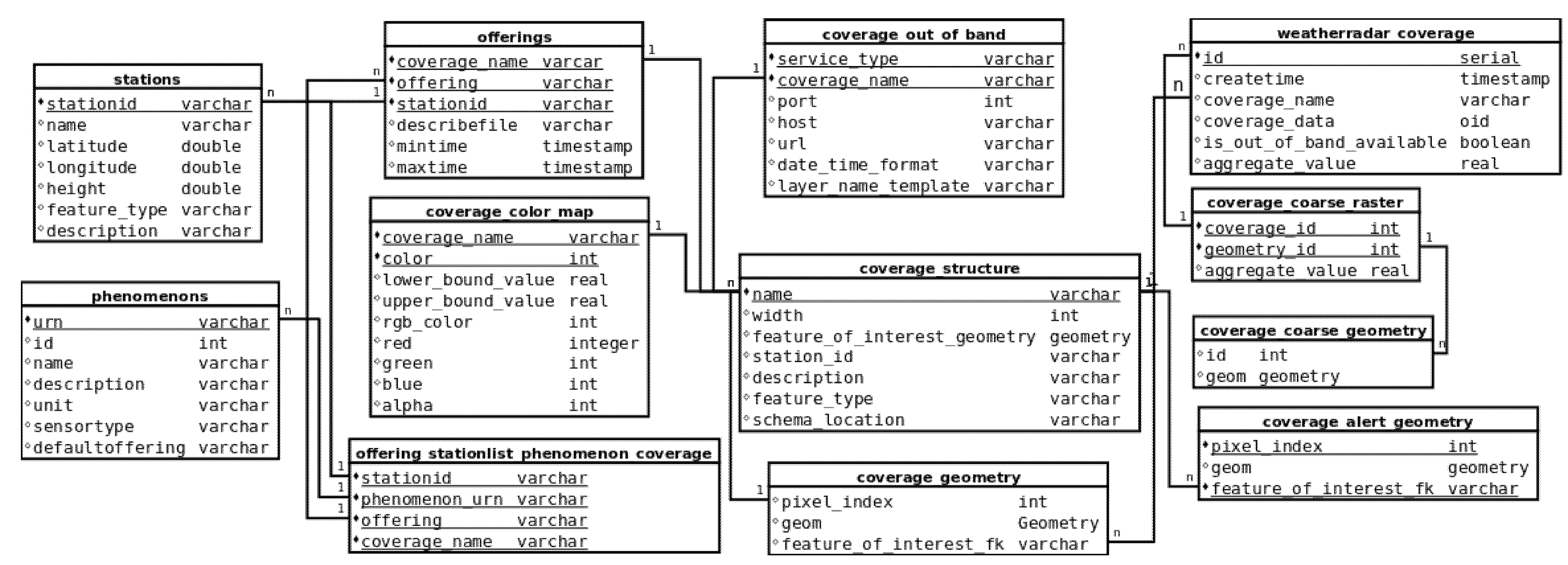
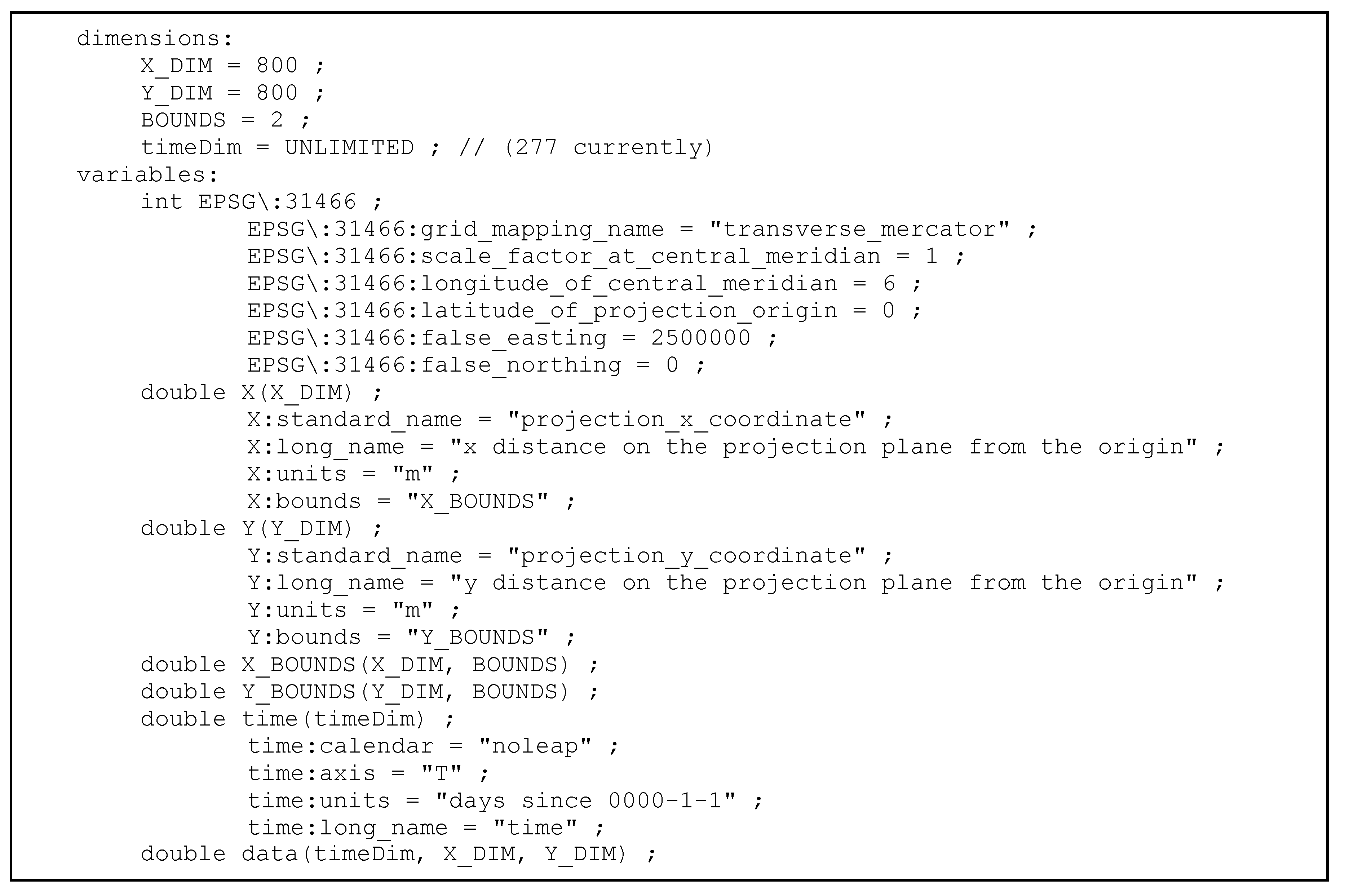
- A data model to store the raster data and its describing metadata in an efficient way has been developed, based on the 52°N SOS data model (see Figure 3).
- •
- Efficient algorithms to apply filters have been implemented.
- •
- Several O&M models to return the raster data in a standardized and flexible manner have been realized.

3.1. Data Model
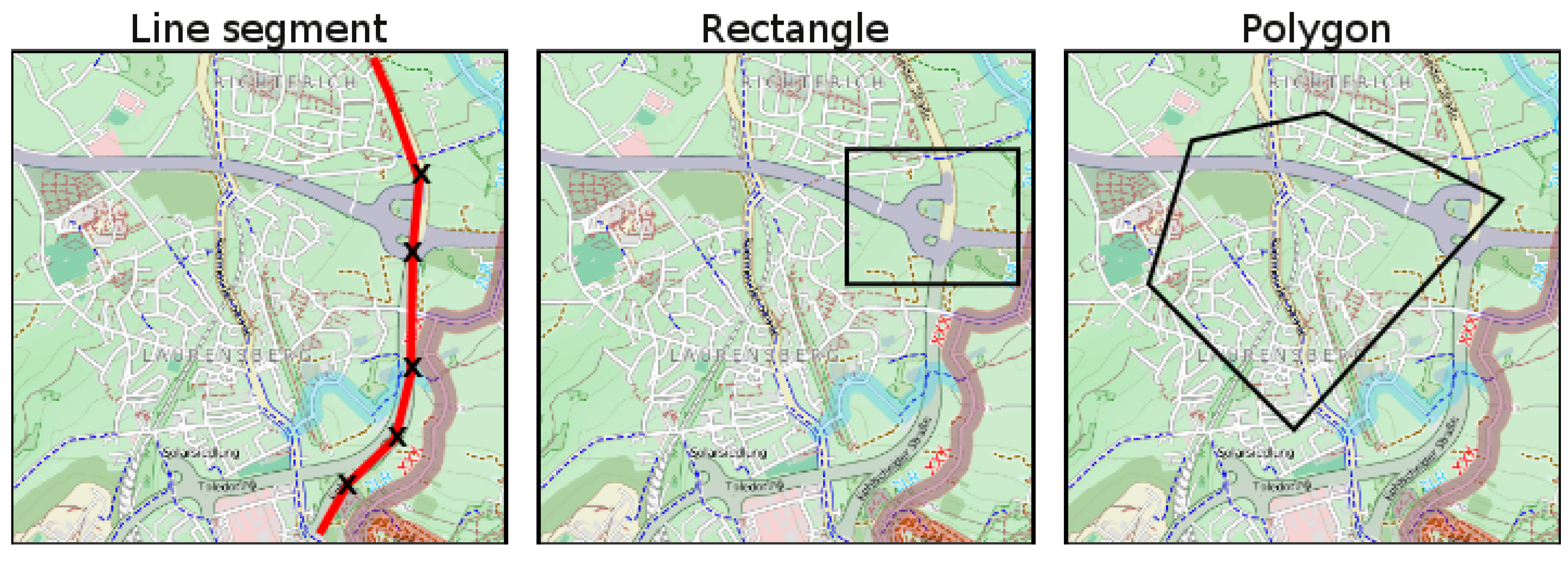
3.2. Filters


| Temporal | Spatial | Thematic | Result |
|---|---|---|---|
| x | -- | -- |  |
| x | x | -- |  |
| x | -- | x |  |
| x | x | x |  |
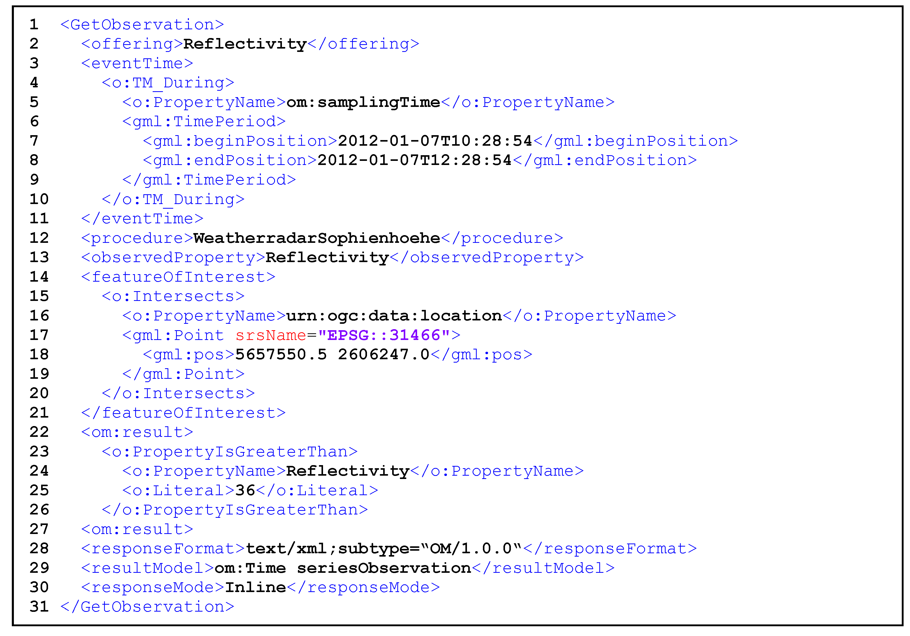
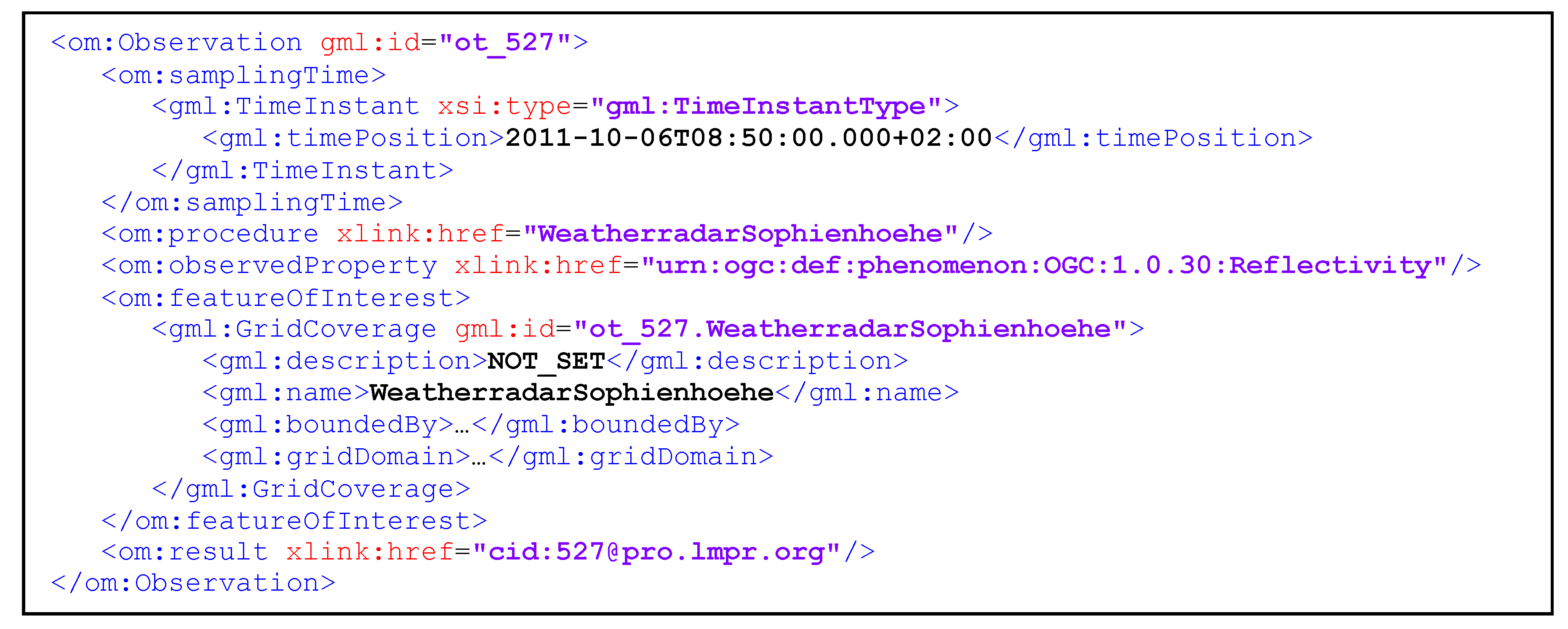
3.3. Result Models


4. Applications
4.1. Data Import
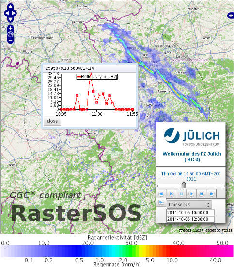
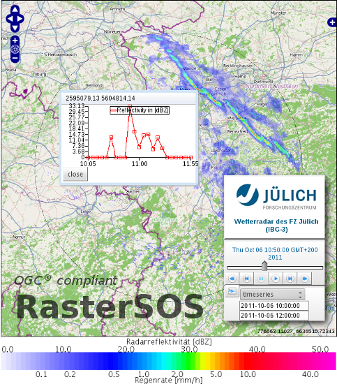
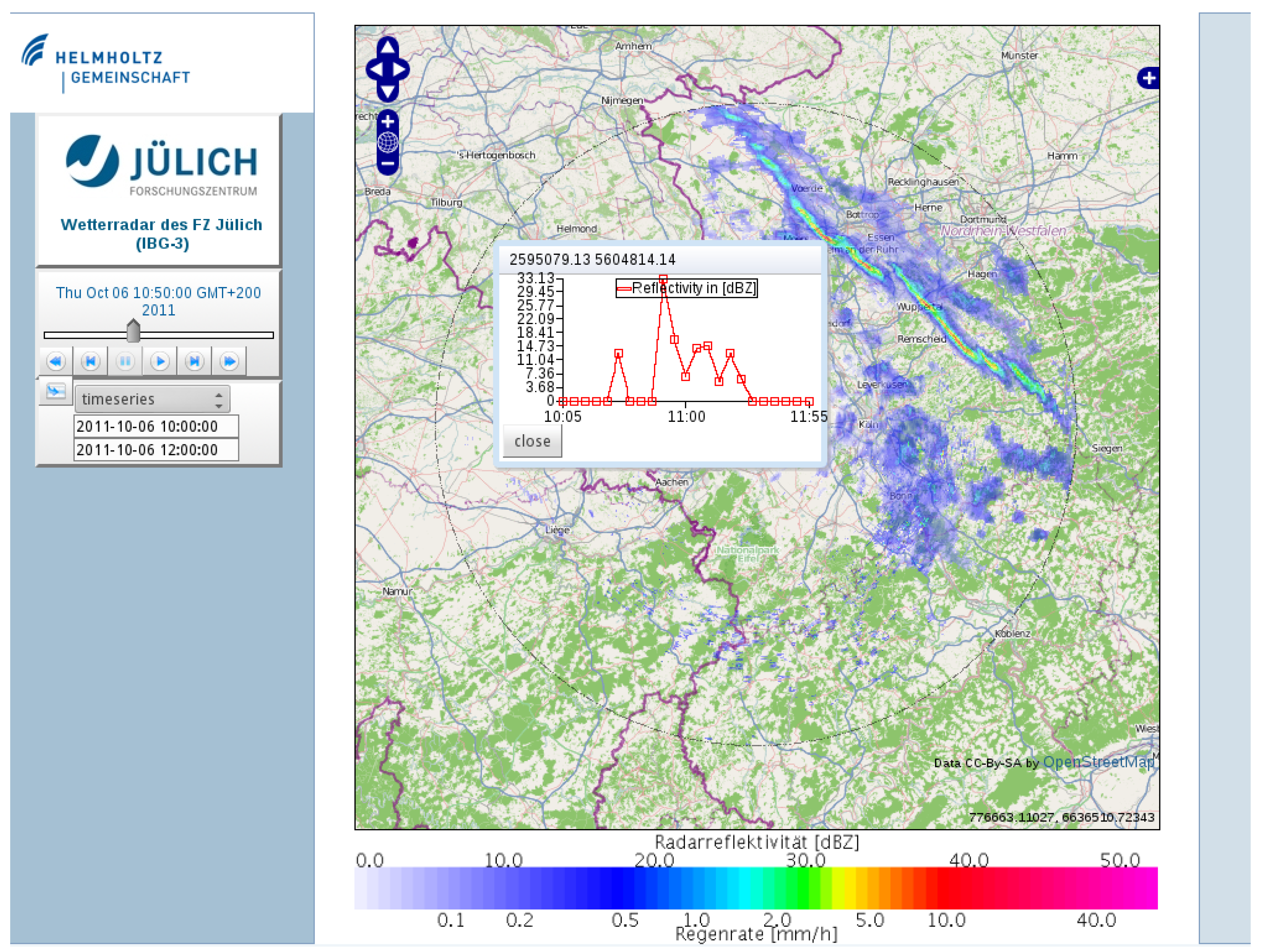
4.2. Visualization of Weather Radar Data


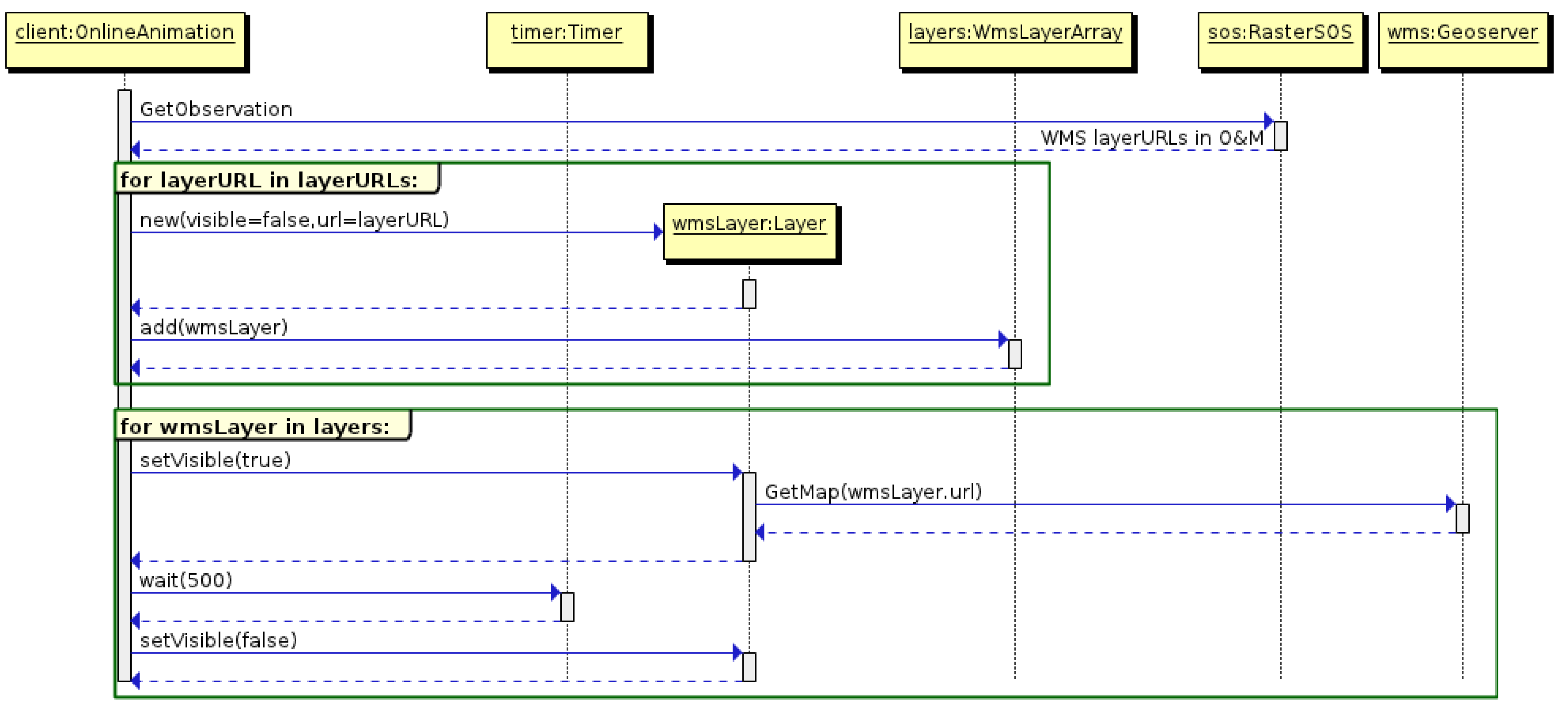
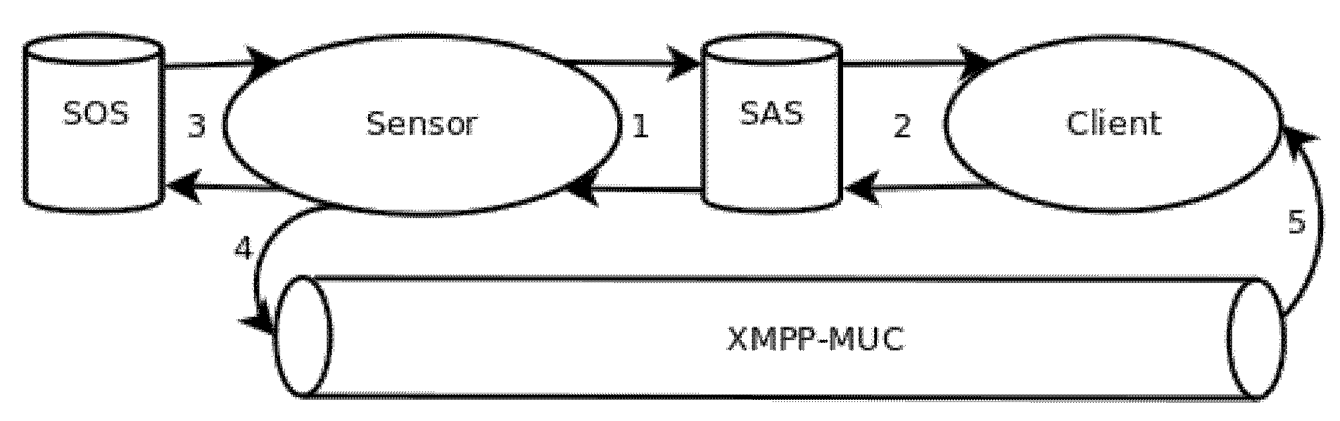
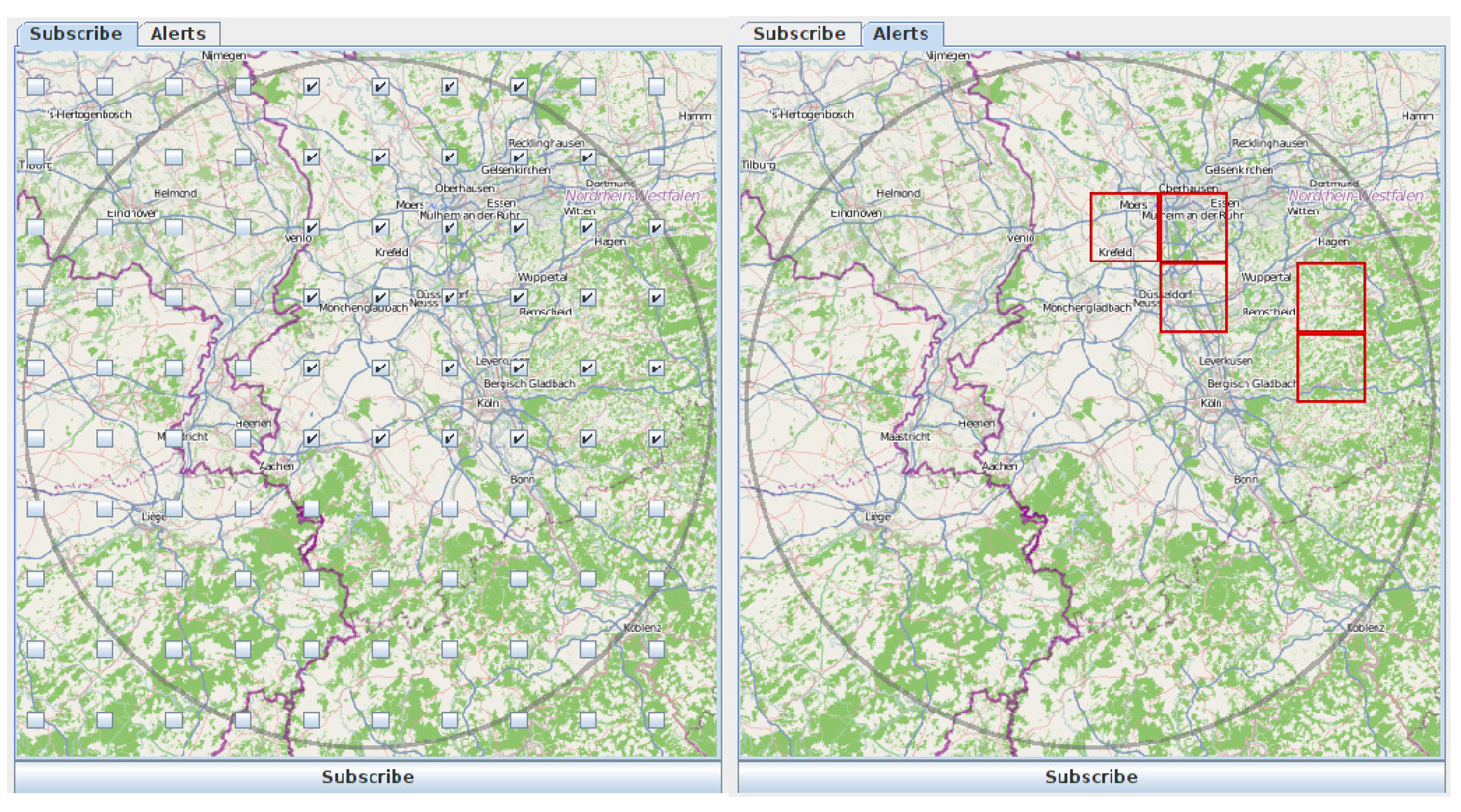
4.3. Client Application for Detecting Heavy Precipitation Regions


5. Results
| Sce-nario | Count | Meshes | Filter | Model | Mode | Format | Net | Time (s) | Size (MB) |
|---|---|---|---|---|---|---|---|---|---|
| 1 | 1 | 640,000 | -- | Om:Discrete-Coverage-Observation | Inline | Plain | Intranet | 600 | 600 |
| 2 | 1 | 640,000 | -- | Om:Observation | Inline | Plain | Intranet | 1.8 | 7 |
| 3 | 1 | 640,000 | -- | Om:Observation | Inline | Zip | Intranet | 1.08 | 1 |
| 4 | 60 | 640,000 | -- | Om:Observation | Inline | Plain | Intranet | 210 | 438 |
| 5 | 60 | 640,000 | -- | Om:Observation | Inline | Zip | Intranet | 200 | 90 |
| 6 | 23 | 640,000 | -- | Om:Observation | Inline | Plain | Internet | 346 | 165 |
| 7 | 23 | 640,000 | -- | Om:Observation | Inline | Zip | Internet | 155 | 34 |
| 8 | 8605 | 640,000 | -- | Om:Observation | Attached | NetCDF | Intranet | 3240 | 365 |
| 9 | 1 | 40,000 | spatial | Om:Observation | Inline | Plain | Intranet | 0.2 | 0.4 |
| 10 | 60 | 40,000 | spatial | Om:Observation | Inline | Plain | Intranet | 12 | 28 |
| 11 | 60 | 250 | thematic | Om:Observation | Inline | Plain | Intranet | 26 | 0.5 |
| 12 | 60 | 1 | spatial (rectangle) | Om:Time series-Observation | Inline | Plain | Intranet | 6 | 0.02 |
| 13 | 60 | 1 | spatial (point) | Om:Time series-Observation | Inline | Plain | Intranet | 0.3 | 0.03 |
| 14 | 60 | -- | -- | Om:Observation | Out-of-band | Plain | Internet | 0.1 | 0.1 |
6. Discussion
7. Conclusions
Acknowledgments
Author Contributions
Conflicts of Interest
References
- OGC. OGC ® Sensor Web Enablement Architecture; Open Geospatial Consortium Inc.: Wayland, MA, USA, 2008; p. 66. [Google Scholar]
- Zacharias, S.; Bogena, H.; Samaniego, L.; Mauder, M.; Fuss, R.; Puetz, T.; Frenzel, M.; Schwank, M.; Baessler, C.; Butterbach-Bahl, K.; et al. A network of terrestrial environmental observatories in Germany. Vadose Zone J. 2011, 10, 955–973. [Google Scholar] [CrossRef]
- Kunkel, R.; Sorg, J.; Eckardt, R.; Kolditz, O.; Rink, K.; Vereecken, H. TEODOOR: A distributed geodata infrastructure for terrestrial observation data. Environ. Earth Sci. 2013, 69, 507–521. [Google Scholar] [CrossRef]
- Bröring, A.; Echterhoff, J.; Jirka, S.; Simonis, I.; Everding, T.; Stasch, C.; Liang, S.; Lemmens, R. New generation sensor web enablement. Sensors 2011, 11, 2652–2699. [Google Scholar] [CrossRef]
- OGC. OpenGIS Sensor Observation Service Implementation Specification; Open Geospatial Consortium Inc.: Mayland, MA, USA, 2006; p. 91. [Google Scholar]
- OGC. OGC® Sensor Observation Service Interface Standard; Open Geospatial Consortium Inc.: Wayland, MA, USA, 2012; p. 148. [Google Scholar]
- OGC. Observations and Measurements—Part 2—Sampling Features; Open Geospatial Consortium Inc.: Wayland, MA, USA, 2007; p. 36. [Google Scholar]
- OGC. Geographic information: Observations and measurements. In OGC Abstract Specification Topic 20; Open Geospatial Consortium Inc.: Wayland, MA, USA, 2010; Volume 2.0.0, p. 57. [Google Scholar]
- OGC. Observations and measurements. In XML Implementation; Open Geospatial Consortium Inc.: Wayland, MA, USA, 2011; Volume 2.0, p. 76. [Google Scholar]
- OGC. Observations and Measurements—Part 1—Observation Schema; Open Geospatial Consortium Inc.: Wayland, MA, USA, 2007; p. 85. [Google Scholar]
- OGC. OpenGIS sensor model language (SensorML). In Implementation Specification; Open Geospatial Consortium: Wayland, MA, USA, 2007; Volume 1.0.0, p. 180. [Google Scholar]
- OGC. OGC® Sensor Alert Service Implementation Specification; Open Geospatial Consortium Inc.: Wayland, MA, USA, 2007; p. 128. [Google Scholar]
- OGC. OpenGIS® Sensor Event Service Interface Specification (Proposed); Open Geospatial Consortium Inc.: Wayland, MA, USA, 2008; p. 88. [Google Scholar]
- Nengcheng, C.; Liping, D.; Genong, Y.; Min, M. A flexible geospatial sensor observation service for diverse sensor data based on Web service. ISPRS J. Photogramm. Remote Sens. 2009, 64, 234–242. [Google Scholar]
- Pfeiffer, T.; Wenk, A. PostgreSQL: Das Praxisbuch; Galileo-Press: Bonn, Germany, 2010. [Google Scholar]
- Obe, R.O.; Hsu, L.S. PostGIS in Action; Manning Publications: Greenwich, CT, USA, 2011. [Google Scholar]
- Holl, S. PostGIS Raster Workshop; FOSSGIS: Dessau-Rosslau, Germany, 2012; p. 18. [Google Scholar]
- Kemper, A.; Eickler, A. Datenbanksysteme—Eine Einführung; Oldenbourg Wissenschaftsverlag GmbH: München, Germany, 2006. [Google Scholar]
- Güting, R.H.; Dieker, S. Datenstrukturen und Algorithmen; Teubner Verlag: Wiesbaden, Germany, 2004. [Google Scholar]
- OGC. OpenGIS® Implementation Standard for Geographic Information—Simple Feature Access—Part 1: Common Architecture; Open Geospatial Consortium Inc.: Wayland, MA, USA, 2011; p. 92. [Google Scholar]
- Broering, A.; Meyer, O. Bereitstellung und visualisierung hydrologischer zeitreihen mit hilfe standardisierter webdienste. In Proceedings of AGIT2008 Symposium und Fachmesse, Salzburg, Österreich, 2–4 July 2008.
- ISO. Geoinformation—Coverage Geometrie—und Funktionsschema (ISO 19123: 2005); DIN Deutsches Institut für Normung: Berlin, Germany, 2005; p. 71. [Google Scholar]
- OGC. OpenGIS® Web Map Server Implementation Specification; Open Geospatial Consortium Inc.: Wayland, MA, USA, 2006. [Google Scholar]
- Kirschke, T. Implementierung eines OGC-konformen WMS als Plugin für einen Geoserver. FH-Aachen: Aachen, Germany, 2012. [Google Scholar]
- Rew, R.K.; Davis, G.P.; Emmerson, S. NetCDF: An interface for scientific data access. IEEE Comput. Graph. Appl. 1990, 10, 76–82. [Google Scholar] [CrossRef]
- Eaton, B.; Gregory, J.; Drach, B.; Taylor, K.; Hankin, S. NetCDF Climate and Forecast (CF) Metadata Conventions. Available online: http://cfconventions.org/ (accessed on 30 January 2015).
- Nativi, S.; Caron, J.; Davis, E.; Domenico, B. Design and implementation of netCDF markup language (NcML) and its GML-based extension (NcML-GML). Comput. Geosci. 2005, 31, 1104–1118. [Google Scholar] [CrossRef]
- Internet Engineering Task Force (IETF). Request for Comments: 2392—Content-ID and Message-ID Uniform Resource Locators. Available online: https://www.ietf.org/rfc/rfc2392.txt (accessed on 13 October 2014).
- Marshall, J.S.; Palmer, W.M. The distribution of raindrops with size. J. Meteorol. 1948, 5, 165–166. [Google Scholar] [CrossRef]
- The PostgreSQL Global Development Group. PostgreSQL JDBC Driver. Available online: http://jdbc.postgresql.org/ (accessed on 30 January 2015).
- Hanson, R.; Tacy, A. GWT im Einsatz : AJAX-Anwendungen entwickeln mit dem Google Web Toolkit; Carl Hanser Verlag: München, Germany, 2007. [Google Scholar]
- Internet Engineering Task Force (IETF). Request for Comments: 6120—Extensible Messaging and Presence Protocol (XMPP): Core. Available online: https://tools.ietf.org/html/rfc6120 (accessed on 20 September 2014).
- OGC. Web Coverage Service (WCS); Open Geospatial Consortium Inc.: Wayland, MA, USA, 2003; p. 67. [Google Scholar]
- OGC. OGC® WCS 2.0 Interface Standard—Core; Open Geospatial Consortium Inc.: Wayland, MA, USA, 2010; p. 45. [Google Scholar]
- Amuthan, G. Spring Mvc Beginner’s Guide Your Ultimate Guide to Building a Complete Web Application Using All the Capabilities of Spring Mvc/Amuthan G; Packt Pub.: Birmingham, UK, 2014. [Google Scholar]
- OGC. OGC® GML Application Schema—Coverages; Open Geospatial Consortium Inc.: Wayland, MA, USA, 2012; p. 35. [Google Scholar]
© 2015 by the authors; licensee MDPI, Basel, Switzerland. This article is an open access article distributed under the terms and conditions of the Creative Commons Attribution license (http://creativecommons.org/licenses/by/4.0/).
Share and Cite
Sorg, J.; Kunkel, R. Conception and Implementation of an OGC-Compliant Sensor Observation Service for a Standardized Access to Raster Data. ISPRS Int. J. Geo-Inf. 2015, 4, 1076-1096. https://0-doi-org.brum.beds.ac.uk/10.3390/ijgi4031076
Sorg J, Kunkel R. Conception and Implementation of an OGC-Compliant Sensor Observation Service for a Standardized Access to Raster Data. ISPRS International Journal of Geo-Information. 2015; 4(3):1076-1096. https://0-doi-org.brum.beds.ac.uk/10.3390/ijgi4031076
Chicago/Turabian StyleSorg, Juergen, and Ralf Kunkel. 2015. "Conception and Implementation of an OGC-Compliant Sensor Observation Service for a Standardized Access to Raster Data" ISPRS International Journal of Geo-Information 4, no. 3: 1076-1096. https://0-doi-org.brum.beds.ac.uk/10.3390/ijgi4031076