Economic Assessment of the Use Value of Geospatial Information

Abstract

Geospatial data inform decision makers. An economic model that involves application of spatial and temporal scientific, technical, and economic data in decision making is described. The value of information (VOI) contained in geospatial data is the difference between the net benefits (in present value terms) of a decision with and without the information. A range of technologies is used to collect and distribute geospatial data. These technical activities are linked to examples that show how the data can be applied in decision making, which is a cultural activity. The economic model for assessing the VOI in geospatial data for decision making is applied to three examples: (1) a retrospective model about environmental regulation of agrochemicals; (2) a prospective model about the impact and mitigation of earthquakes in urban areas; and (3) a prospective model about developing private–public geospatial information for an ecosystem services market. Each example demonstrates the potential value of geospatial information in a decision with uncertain information.

1. Introduction

Geospatial information is a form of infrastructure for decision-making that supports many societal activities. The cost of supplying the information is greatest to the first user; the cost of disseminating information to additional users is relatively small. This is true for most information goods [1] and is referred to as jointness of supply. This characteristic gives rise to the need for studies to demonstrate the value of the information (VOI) or the benefits of the information. The benefits are best demonstrated when analysis can explain how the data are used in a decision.

Most VOI analyses consider the costs of geospatial data collection and the potential cost savings to society accruing from the presence (rather than absence) of geospatial data. This type of analysis can be referred to as cost-savings applications. There also are societal benefits that can result from making more informed decisions. Analyses measuring this type of benefits can be referred to as innovation applications. Both types of applications can be pursued with the systematic availability of archival and current geospatial data that result from open access to replicable, and continuous data frameworks that do not exclude anyone from the benefits of its use.

Both cost-savings and innovation applications are used to document the expected use value of information. Geospatial and spatiotemporal public data are integrated into current economic activities that have considerable economic benefits such as transportation route and communication facility planning. Economic models have been developed to estimate the benefits of geospatial data for a wide range of topics in industrial sectors such as agriculture [2,3,4,5], resource extraction [6], environmental hazards [7], wildfire management [8] and maritime shipping [9].

Here we focus on innovation applications for geospatial data. The approach is driven by the information, which involves examination of spatial and temporal scientific, technical, and economic data. The observations evolve into spatiotemporal patterns that are used to identify and test hypotheses for how geospatial information is integrated into decisions. Economic models then can be used to estimate a gain in societal welfare that results from making better decisions that are based on additional information in the presence of uncertainty. The societal gains from the additional information depend on the reduction in uncertainty that is offered by the additional information and what is at stake in the decision. The approach taken here is based on explicit modeling of the change in the decision maker’s information and the implications of that change on the decision maker’s objectives and constraints. Although decision makers have some information, the decision framework must be able to describe how the decision maker’s information changes as a result of the acquisition of new information to update prior beliefs, i.e., a use value. Thus, a decision maker’s updated belief will affect their decision and the benefits of a choice.

Below we describe three applications. Each example illustrates the steps in the analytical process. Two of the analyses employ geospatial data and information in decision frameworks that provide examples to demonstrate the potential for a significant return on investment in geospatial data collection and distribution. The third application is a potential application to markets for ecosystem services that can be based, in part, on multiple scale public/private sector integration of remote sensing and other geospatial data.

The example applications are set in the context of valuing the vast array and amount of geospatial data that are associated with the open access. For the economic foundation, we assume that geospatial information is a technical innovation and apply microeconomic theory in an inductive process [10]. Our approach is to examine data, identify a pattern in the data, propose and test a tentative hypothesis, and establish a generalization or theory. For example, the inductive approach is found in agent based computational economics [11].

Monetary values are established in specific applications in an empirical economics approach as the basis for the use value of the information. The method has two stages. The first is the development of an interdisciplinary model of economic behavior in which the application of the geospatial information is demonstrated as a consequence of spatiotemporal observations. The second stage is to compare the net benefits with and without the geospatial information to estimate the VOI. In this paper, we only address estimation of the economic value of geospatial data used for decision-making.

Geospatial data are collected and distributed in many ways, all of which require a significant investment in science, technology, operations, and administration. Geospatial information can be used in an inductive mode to examine large data sets to reveal relationships and dependencies and to perform predictions of behaviors and outcomes [12]. The remainder of this paper establishes the context for the introduction of models to estimate the economic benefits of open access to public data and the emerging market for private data. The next section is a brief introduction to an economic model to value geospatial information as a technological innovation. Three examples follow the model. Example 1 is an inductive retrospective model about environmental regulation of agrochemicals that negatively impact potable groundwater resources. The application demonstrates how geospatial data can provide information for regional health policy decisions. Example 2 is an inductive prospective model about the impact and mitigation of earthquakes and the influence of regional income distribution. A simulated earthquake provides geospatial information for understanding dynamic physical processes and their effects on specific income groups in urban areas. Example 3 is about developing private–public geospatial information as a baseline and measure of the change in emissions and pollution in an ecosystem market approach as a way to help align economic incentives. The application of geospatial information reduces market transactions costs. The last section is a summary.

2. Estimating the Economic Impacts of Geospatial Technology: A Model of Technological Innovation

Most publicly provided geospatial data (specifically U.S. unclassified data) are accessible without any restrictions for usage and distribution. Data creation and distribution is a technical activity. Open access to publicly delivered data introduces a way to implement integrated models that can be used for policy, regulatory, and market decisions. Implementation requires transforming geospatial data into information that then gets adopted and acted on by decision makers. The transformation from data to action is a cultural activity [10]. Starting with examination and analysis of available data, we propose a model of economic change as a result of technological innovation. Examination and analysis includes some form of data mining, inference, and prediction of a pattern of economic or social activity. For geospatial information to be included in decision processes, it has to be demonstrated that the data add value to the decision taken.

Formally, geospatial information is an intermediate economic good that has a significant role in private and public decisions. That is, the consumer of the geospatial information has a derived demand for the data [7,13]. Geospatial information is a fundamental input to reducing uncertainty in decisions. The VOI of geospatial data is the economic value added resulting from more informed decisions that are based on incremental increases in information in the presence of uncertainty. VOI depends on (a) what is at risk at being lost as an outcome of a decision and (b) the effective decrease in decision-makers’ uncertainty(ies).

Geospatial data are a private good when considered specific information that supports individual firm and industry decisions. In the context of maps, “specific” refers to information that is localized and narrow in focus [14], (see [7] for an application). As the information becomes more specific, the range of applications becomes limited, and the number of actual and potential users is small. Monitoring groundwater mitigation measures for acid leaching at a coal strip mine provides a good example. In compiling “specific” information for efficient business operations, it is often necessary to locate and prioritize specific targets.

Geospatial data are a public good when it is “general” information and refers to information collected at a scale pertinent to a variety of regional decisions [7]. General geospatial information has two characteristics: (1) it is impossible or inefficient to exclude anyone from consuming the good once it is produced. That is, the information is nonexclusive in consumption; any one individual’s consumption of the output does not reduce the consumption by others. (2) The production of the information is characterized by jointness of supply. Economic efficiency is achieved when the cost of production is equal to the market valuation of the good for the last unit produced. If the marginal cost is zero (all costs are fixed and would be incurred whether 1 unit or 100 units are produced), economic efficiency dictates that the good be “sold” at 0 price, i e., be made freely available [7]. Generally, the information can inform and/or influence decisions involved in mineral exploration, waste repository site selection, recreational and conservation designation, establishment of ecological preserves, residential and commercial construction, and many others (Although most geospatial data are public data in the U.S., this may not be the case elsewhere.). Given the slow rate of decay of its usefulness, such information has a long life span and there is a lack of congestion costs (one individual’s use of the information does not degrade its value to another). There are specific circumstances where geospatial may decay rapidly such as locations of shelters following a specific disaster. However, even in this example, a spatial archive of previous actions can be used to avoid mistakes in disaster recovery in future hazards.

An inductive economic model is used to identify and develop specific applications for analysis of economic benefits. The inductive method is an empirical method of economic analysis in which statistical characteristics of the data serve as the basis for generalizations [15]. The inductive approach can be employed to verify the conclusions of economic theory formulated by the deductive method. Because inductive procedures substantially work with statistical tools, there is the potential for accomplishing results that are nearer to reality, and as the sample size increases and there is a good statistical representation of the data, the exactness of the outcome improves. In the examples below, geospatial information is generalized and cases made about the economic benefits of investments in a series of technological innovations that enhance society’s productivity. As the product of innovation, geospatial observations and in use analyses are views of activities that produce goods and services at a place and time in a region for markets.

When an economy is operating efficiently, production is at a maximum for a given set of inputs. Any changes in the outputs of the region are production tradeoffs given the fixed amount of resources. A regional production possibility frontier (PPF) curve shows the maximum possible production level of one commodity for any given production level of another, given the state of technology. In estimating a dollar value of geospatial information, it is assumed that the market is competitive. Because the requirements for a functioning competitive economy are achieved, the joint output of the economy for a production scenario is a point on a production possibility frontier (PPF) in Figure 1 [2]. Figure 1 illustrates one application of this approach that has been applied to evaluate different estimates of efficient outcomes of the joint output of an economic activity (crop production) and its impact on an ecosystem service (potable groundwater). The different outputs for the goods can be plotted along a PPF for a set of policies. The geospatial data are a technological innovation that when applied to a current land use allocation, create an outward shift in the PPF from PPF₀ to PPF₁. The result is that society can have a more valuable mix of economic production and the sustainability of an ecosystem service. The economic value of geospatial information is derived from the outward shift in the PPF in Figure 1.

Figure 1. A production possibility curve for a technological innovation in geospatial data (source: [2]).

Figure 1. A production possibility curve for a technological innovation in geospatial data (source: [2]).

Three examples of the inductive model are presented below. The first example is a retrospective model about environmental regulation that includes both an interdisciplinary model of economic behavior and an estimate of the VOI (net benefits). The second example is a prospective model of a science-based local ordinance for mitigating a natural disaster. The first stage of applying the inductive model has been completed. The third example is in the examination phase. An economic model is proposed for the first stage of the inductive model. The inductive approach follows a series of steps that are the basis for the procedure to estimate the net benefits of an investment in technology:

(1)

Decide whose benefits and costs count and identify relevant geospatial data and information;

(2)

Determine the potential impacts and select measurement indicators;

(3)

Predict the quantitative impacts of the project;

(4)

Monetize all impacts at a discount rate to estimate the net present value of the benefits of the project;

(5)

Estimate the net benefits and perform sensitivity analysis.

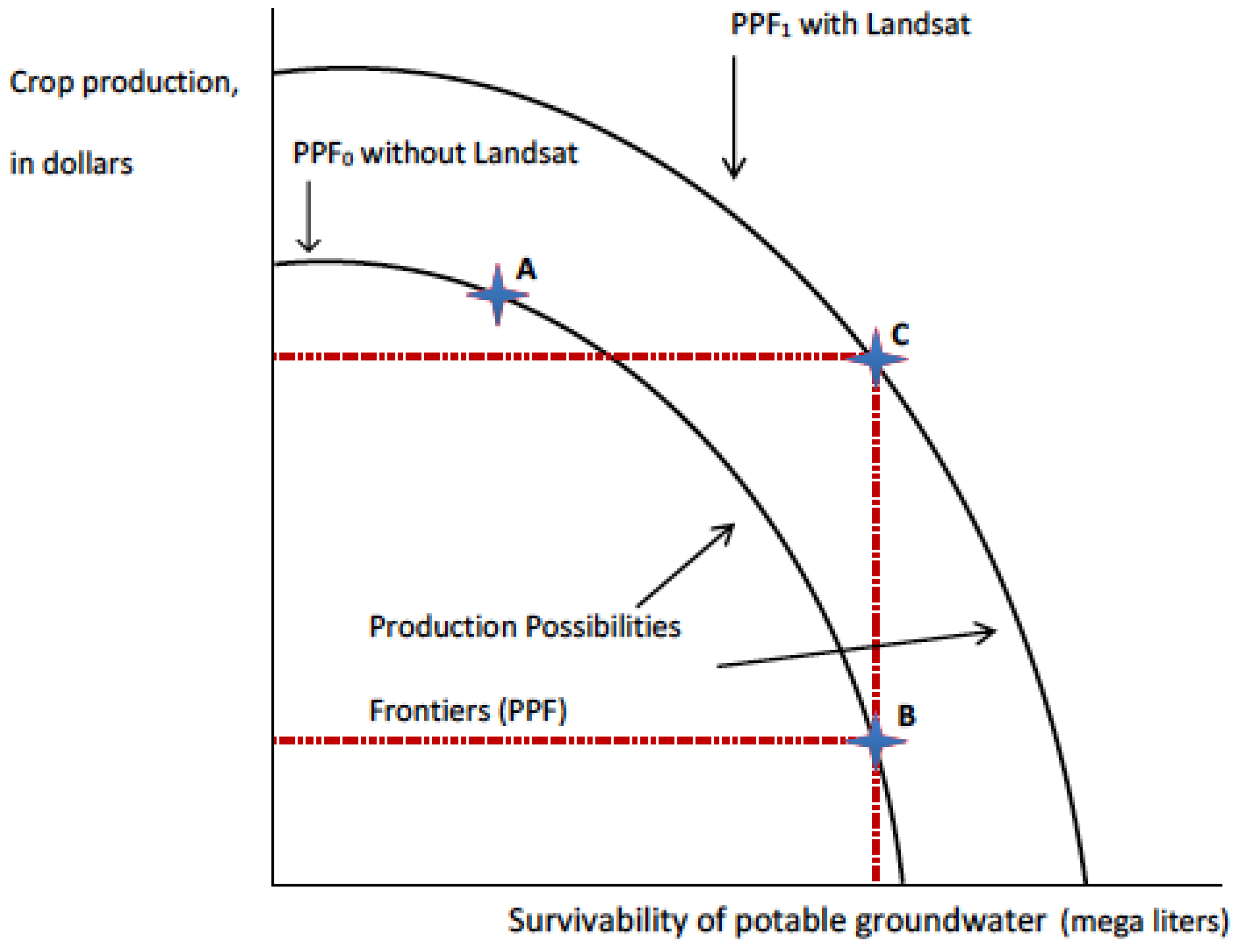
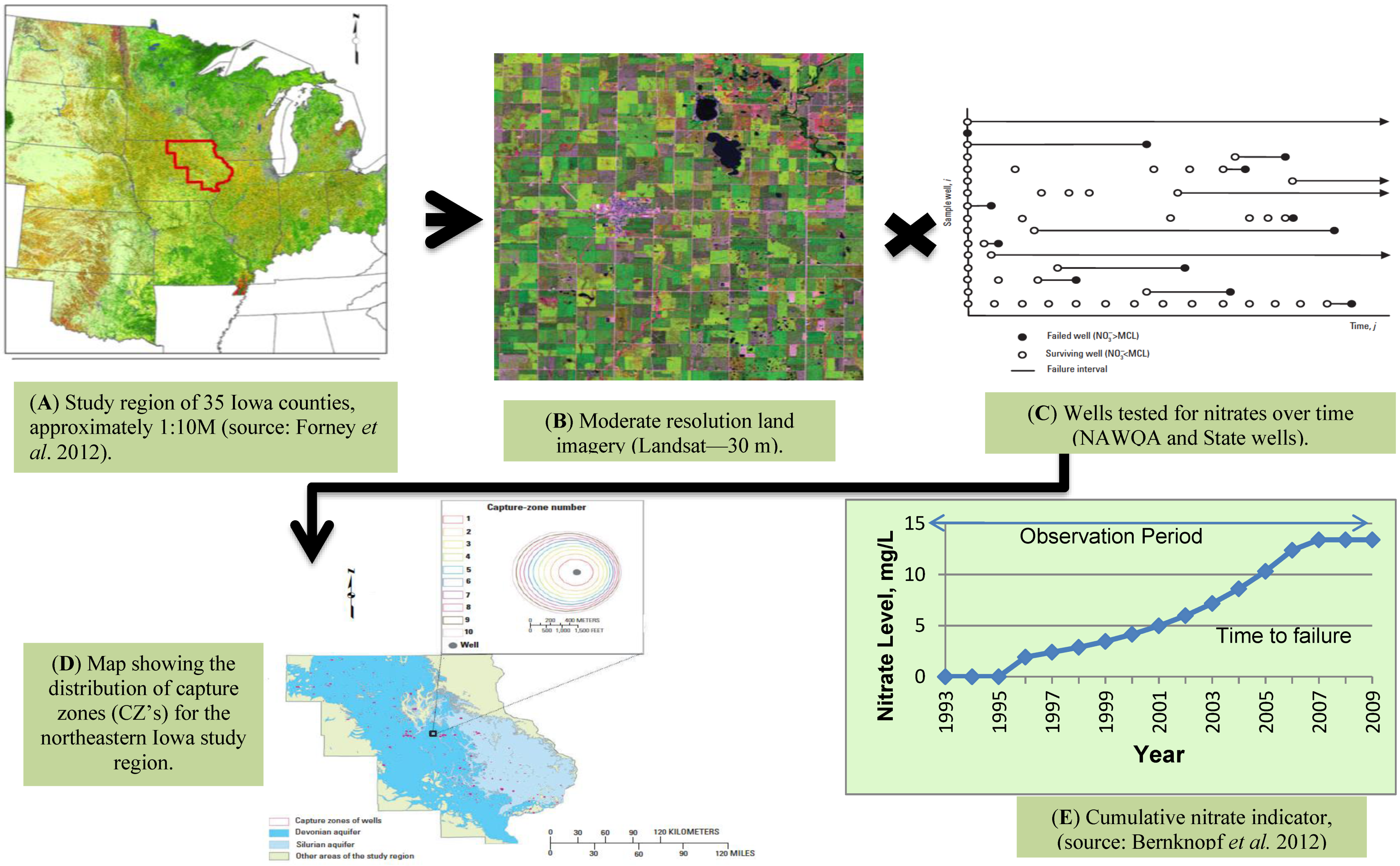
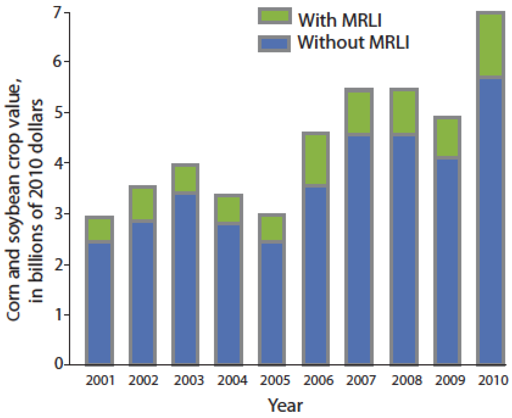
3. Example 1. An Inductive Retrospective Model—Environmental Regulation of Agrochemicals: Geospatial Data Provide Information for Regional Environmental and Health Policy Decisions

This example is a retrospective model for estimating the benefits of moderate resolution land imagery (MRLI) as open access geospatial data. MRLI is spatial data having a pixel resolution between 30 and 250 meters. Land use and land cover data for the Earth has been updated regularly since the 1970’s. Here MRLI accrues benefits to society by providing a spatiotemporal land use/land cover (LULC) signal that can be linked to ground-based, land management activities and their impacts on human and natural ecosystems [16]. The societal benefit of the MRLI information is the increased efficiency in government regulation. Cost savings arise from avoiding costly errors in administering regulations concerned with groundwater contamination for compliance with the U.S. Clean Water Act. Samples of decisions are: to shut down a drinking water well because it has exceeded the drinking water quality limit, to transition the well to one for irrigation supply rather than drinking water, or to have regulators miss high levels of nitrate (NO₃⁻) concentration in a well therefore resulting in costly adverse health impacts. MRLI sensors and their data archives provide information at a derived error rate in detecting farm land use that can be used as an input to a probabilistic estimate of an adverse change in water quality. The example demonstrates how MRLI provides a cumulative accounting of crops that have differential impacts on groundwater quality. Combining the MRLI and a groundwater vulnerability model is used to forecast critical levels of NO₃⁻ concentration in an aquifer over time. These data can inform decisions to regulate land use for mitigating a potentially loss of drinking water by imposing constraints on the farmer’s practices that might reduce their output.

The environmental regulation application requires a conversion of earth observations into an input to decisions to regulate the application of a nutrient to crops that potentially could contaminate regional groundwater supplies [2]. The VOI issue is whether decisions are better informed for the individual farmer(s) and regulators with spatiotemporal MRLI information [16]. The baseline in this example is for the farmer and regulator to rely on the current and historical groundwater well records and inspections of ad hoc and variable data of agricultural land uses.

3.1. Background

Geospatial information was used to identify places over a 10-year period where agricultural production may have required nitrogen fertilizer, which can contaminate groundwater. The USEPA health standard states that nitrate in drinking water cannot exceed 10.0 mg/L. Exceeding the standard has been linked to multiple types of cancers, disruption of thyroid function, birth defects, methemoglobinemia (“blue baby syndrome”) and hypertension; other adverse health impacts including miscarriages and cancer risks were noted in populations with drinking water with nitrate levels higher than 2.46 mg/L.

Archival land use information contained in the USDA Cropland Data Layer (CDL) was linked to a regional groundwater vulnerability model [2]. The CDL based on MRLI provided corn and soybean production estimates for 2001–2010. The geospatial information was coupled to earth science process models to assist in decisions about land uses and their impacts on groundwater supplies. For example 80% of Iowa drinking water is from groundwater.

Figure 2. (A) Landsat image covering 35-county study region in Iowa, (B) Landsat image of parcels, (C) Illustration of arbitrarily interval-censored data used in the statistical survival model, (D) Regional map of wells and capture zones, and (E) Graph of nitrate accumulation over time for exceeding the regulatory standard (source: [2]).

Figure 2. (A) Landsat image covering 35-county study region in Iowa, (B) Landsat image of parcels, (C) Illustration of arbitrarily interval-censored data used in the statistical survival model, (D) Regional map of wells and capture zones, and (E) Graph of nitrate accumulation over time for exceeding the regulatory standard (source: [2]).

The study was conducted in a region that covered 5.4 million hectares in 35 Iowa counties shown in Figure 2A where corn (average application of 114.2 lb/acre of N) and soybean (average application of 3 lb/acre of N) are the major crops. The integrated model covered 603 watersheds (subbasins) with a median of 7910 Hydrologic Response Units (HRU). HRUs are areas within the region’s watersheds that respond similarly to a given input and contained 32,000 wells ranging from just below the surface to 1220 meters in depth. Figure 2B is a more detailed image of MRLI that shows parcel land cover and land use in a specific area in the region. With ten years of observations over the same territory it is possible to identify the agrochemical application rates for estimating the mobility of N into soil. The graph in Figure 2C illustrates the considerable variability in the fate and transport of agrochemicals between the ground surface and the primary aquifers used for drinking water. Contamination of groundwater occurs at different rates and at different times across the region. The regional map in Figure 2D shows the distribution of water wells in the study region and a well capture zone (CZ) for calculating annual nitrate loading.

Each water production well has a surface area that is considered the wellhead protection zone that delineates a time-of-travel capture zone for the well over time [17]. Individual CZs around specific wells contribute to the fate and transport dynamics of nitrate observed in wells [2]. Using the delineated CZs and the MRLI observations, the area under various land uses in the CZs of wells is used to quantify the amount of nitrates contributing to groundwater pollution. CZs for particular wells in the insert map in Figure 2D shows the CZ’s for a particular well and their annual location during a 10-year period. Over the period of analysis there is an accumulation of nitrate pollution that has moved through the hydrogeologic system and, observed over time in a given well for its CZ. The NO₃⁻ concentration at a well might increase through time because of an increasing proportion of its “capture” area that might be devoted to agriculture or because of an increase of corn vs. soybean cultivation through time. It might also increase through time because of a progressively reduced capacity for NO₃⁻ reduction along the relevant hydrologic flow paths. This movement is modeled as a difference equation referred to as the cumulative nitrate indicator (CNI) [18,19]. The CNI uses the measured nitrate level in the current and previous time periods and the addition of nitrate to the existing pool or amount in the given year from the nitrogenous fertilizer applied over the defined period of time. The difference equation estimates the annual change or the dynamics of nitrate concentration over the given time period. The graph in Figure 2E is an illustration of accumulated nitrates over time.

Drinking water well survival is defined as the groundwater nitrate concentration within the limit of the maximum contamination level (NO₃⁻ < MCL) and failure when exceeded (NO₃⁻ > MCL). Groundwater samples that were collected and chemical analyses of the samples indicated either the well was a surviving well or a failed well, thus isolating time intervals in which the failure occurred as shown by the solid lines [2]. The pattern that emerged from the data about well failures, surficial geology, depth, and other physical variables was input into a statistical regression model and then used in a statistical survival model. This last step demonstrates the support and benefits the earth observations provide in converting seemingly unrelated data sets to a measure of environmental health risk.

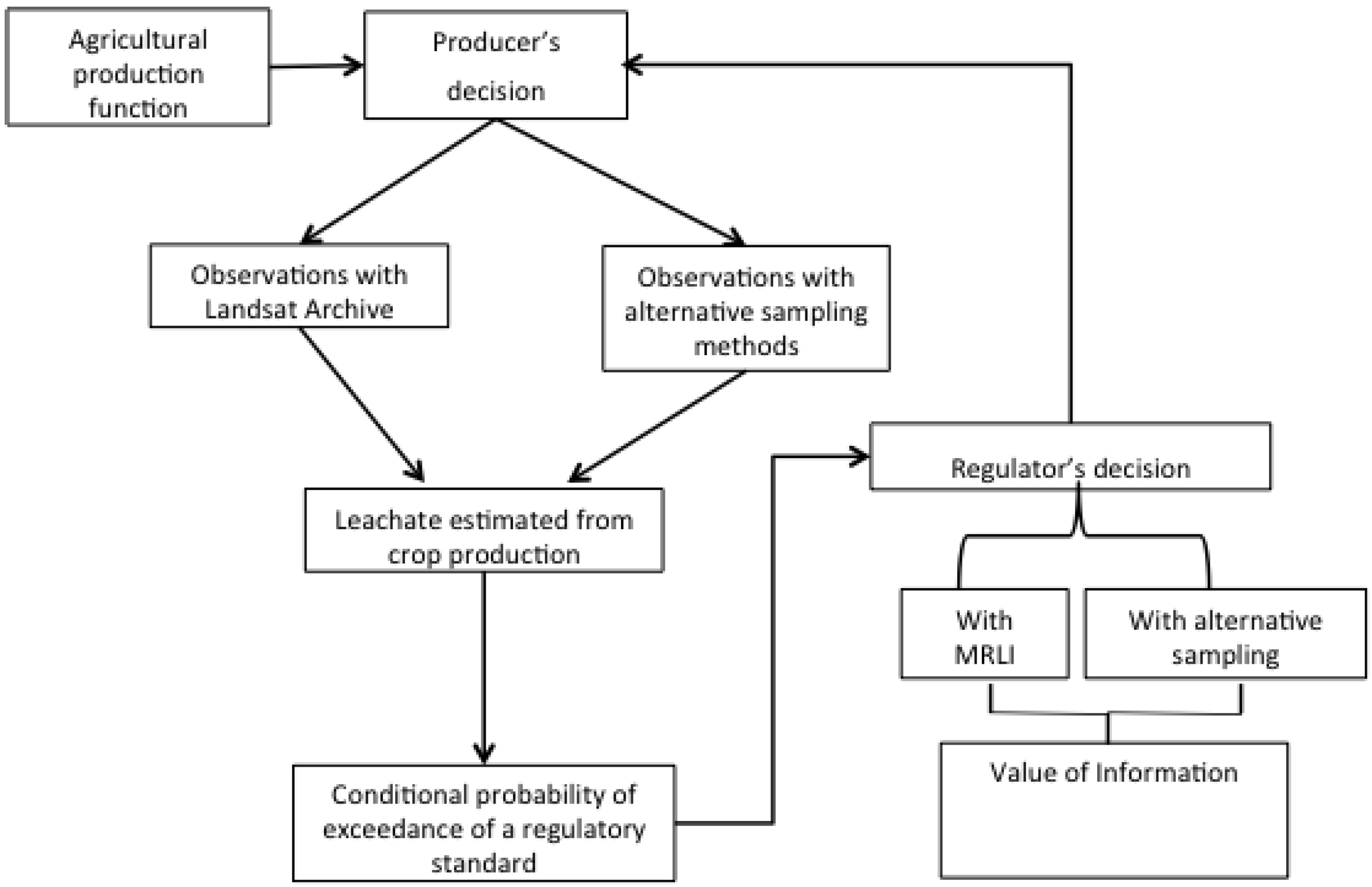
3.2. Analysis

The integrated modeling approach combines agricultural producers and environmental regulators in the decision processes, while using information from markets and natural systems to aid in the objective [13]. Trade-offs between development and preservation preferences are central to the model. The tradeoffs can be shown by using Figure 1 to explain what happens with and without MRLI. Points A and B on PPF₀ represent two efficient allocations of land corresponding to two different levels of crop production and survivability of potable groundwater wells (see [2] for more details about the economic model). Point A represents a regional economy that has a high level of crop output and low survivability of potable groundwater. Point A maximizes crop production given a particular level of surviving, potable groundwater. Point A could be current and historical crop patterns from the CDL. Alternatively, point B represents a regional economy that lowers the risk of losing potable groundwater for a given lower level of crop production. Points A and B are alternative optimal solutions of regional land allocation without MRLI. Point C on PPF₁ improves the regional allocation of land with MRLI (Landsat) by taking advantage of the technological advances in Earth observation. Point C is a reallocation of land use based on the examination of MRLI data and translation of the data into a classification of land use that is linked to models of groundwater vulnerability. The improved classification allows identification of better locations for particular land uses (Of course trying to actually use the information to change land-use can be politically problematic). The additional information may allow regulations to be better targeted so that crop production can be increased while keeping the quantity of potable water remain the same (at point C on PPF₁ in Figure 1), thereby realizing the economic value of MRLI data.

The economic value of the change in the quantities produced for each crop (corn or soy) is the basis for the application of estimating the benefits of MRLI. The present discounted value for the range of years analyzed is calculated by summing the quantities of corn and soybeans produced in each land unit into a time series and multiplying by the discounted real prices that prevailed during the period of analysis. Cropping choices over location and time across the study region are eliminated if the environmental constraint is exceeded. Among those choices not eliminated, the model is used to identify cropping choices until a maximum economic value is identified and annualized [2]. The present discounted value of the difference between optimal (with MRLI and associated modeling data) and baseline (without MRLI data) is each crop price times the change in crop quantity. The VOI is expressed as an equivalent annual income. Assuming a similar flow of benefits into the future because of the continuation of the availability of MRLI, for this region is the net present value.

The conceptual framework in Figure 3 outlines the natural science—economics decision model and procedure for VOI estimation [16]. In the framework the farmer’s objective is to maximize profit subject to environmental regulations and land characteristics and the regulator’s objective is to maximize total revenue subject to environmental risks not exceeding the existing health standard. The geospatial information was input to a probabilistic model of groundwater vulnerability. Spatiotemporal statistical information was used to convey time-dependent nitrate accumulation at water wells. Along with land and geologic characteristics the model was used to estimate how long well water for the next 10 years (2011–2020) would survive below the health standard and serve the public. The probability of survival for each HRU for 2011–2020 was applied in a regulatory decision to evaluate the different impacts of intensive and extensive agricultural land use. Intensive agriculture is differentiated from extensive agriculture by higher transformative inputs (e.g., capital, labor, agrochemicals) relative to land farmed. Extensive agriculture produces a lower yield per unit of land, and therefore generally requires large quantities of land in order to be profitable [20]) while maintaining future groundwater quality. For the model the following three assumptions were made: (1) land use has been and will remain in agriculture during the period of analysis, (2) the nitrate standard of 10 mg/L will remain in effect for the foreseeable future and, (3) consumers and producers expect the future to be reasonably consistent with the past in the regional economy.

The statistical model was a proportional hazards model used to estimate the probability of well survival. The estimate depends on the number of years that elapse from any point in time a well is found to be in the “surviving” condition. The map in Figure 4 shows the distribution of groundwater survivability in the study region and the probability of survival for three specific wells. The probabilistic model is used to decide whether to continue using the well for drinking water. In the example the condition for a well failure is a 0.01 chance of exceeding the MCL for nitrate at each of the wells in the region. Dynamic nitrogen loading and transport at specified distances from specific sites (wells) and at landscape scales was simulated for 35 Iowa counties and two aquifers.

Figure 3. Conceptual framework for producer and regulator choices for estimating the monetized benefits of moderate resolution land imagery (MRLI) (source: [16])

Figure 3. Conceptual framework for producer and regulator choices for estimating the monetized benefits of moderate resolution land imagery (MRLI) (source: [16])

Figure 4. Map of groundwater failure and estimated subbasin probability of survival. The graph replicates the probability of survival for 3 wells, which depends on the number of years elapsed when a well is found to survive below the regulatory threshold (source: [2]).

Figure 4. Map of groundwater failure and estimated subbasin probability of survival. The graph replicates the probability of survival for 3 wells, which depends on the number of years elapsed when a well is found to survive below the regulatory threshold (source: [2]).

3.3. Results

In this retrospective analysis, MRLI contributes to decision making as a revision of regional land use by reassigning crops to parcels by changing the corn/soybean distribution in space and time that will maximize the value of agricultural production and preserve potable groundwater resources. The impact of the geospatial information for the management of the production of corn and soybeans and their effects on groundwater quality is significant. Figure 5 shows the annual change in the values of the two crops after the rearrangement of the land use to avoid any further groundwater contamination. The differences in the economic values during the 10 years of the study are due to the quantities harvested and the relative prices of corn and soybeans. Evaluation of the model outcomes for the 10-year period of analysis from 2011–2020 suggested that some groundwater wells are threatened by nitrate contamination and could fail to maintain drinking-water quality. Other locations are where the topography, soils, well characteristics (such as depth and operations), and surficial geology are less likely to transport the contaminant to the water supply.

Figure 5. Bar graph showing the annual flow of economic benefits (2001–2010) with and without the availability of MRLI for the 35-county northeastern Iowa region (source: [21]).

Figure 5. Bar graph showing the annual flow of economic benefits (2001–2010) with and without the availability of MRLI for the 35-county northeastern Iowa region (source: [21]).

The VOI is estimated as (1) the economic benefit stream of a net increase in agricultural production across a region without sacrificing groundwater resources and (2) how agricultural production and its environmental impacts may change with or without the availability of MRLI. For the 35 counties in northeastern Iowa the estimated VOI for MRLI is an annualized $858M ± $197M/yr (in $2010) and has a current value of $38.1B ± $8.8B for that flow of benefits into the foreseeable future [2]. These estimates assume that all the land parcels are reassigned with no transactions costs or regulatory restrictions. A full policy analysis was beyond the scope of the study; instead, tools were developed to calculate the highest value possible using MRLI information. This includes an abstraction regarding the policies that realistically could be used to achieve a possible increase in value. More conservative estimates involve policy and financial value judgments. A conservative (more realistic) rate of land use change that yields a 1% improvement in land allocation has an estimated VOI for MRLI of an annualized $43M/yr (in $2010) and has a net present value of $1.91B for the 35 counties in Iowa. 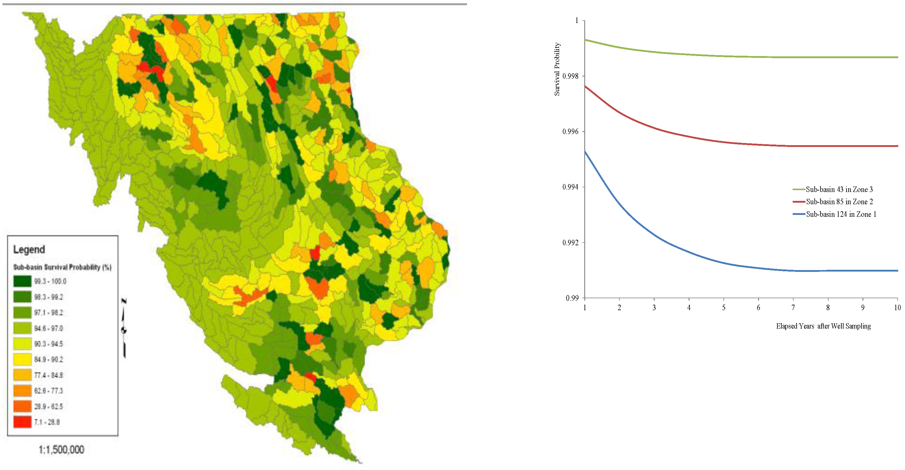Thus, the results can be adjusted downwards to reflect specific policies.

3.4. Summary

In the example, MRLI provides the full population of land uses, while traditional techniques might less frequently sample a subset of land uses, thereby providing less information. The MRLI facilitates spatiotemporal analysis of the impact of nitrates on groundwater resources. The geospatial information archive is critical because groundwater pollution accumulates from nonpoint sources over a period of time. The archive provided the data to identify a pattern of land classified into specific crops in the USDA Cropland Data Layer and a link to samples of nitrate levels found in water wells years later. This information was input into a statistical survival model to estimate the time-dependent probability of exceeding a health standard. In the example the economic benefit of the geospatial data derives from informing the management of corn and soybean crops and the impact on soils and groundwater. The value provided by MRLI can be estimated by the incremental benefit of increased revenue from land with the use of MRLI without further deteriorating groundwater quality. The focus of the analysis was on the use of improved information (from MRLI) to estimate the joint production of agricultural goods and environmental impacts. The information provides the capability to monitor all agricultural production at parcel level with high accuracy (average greater than 95% accuracy for 2000–2010; see Table 2, p.24 in [2]) while keeping the constraints posed by the US EPA drinking water level for nitrate.

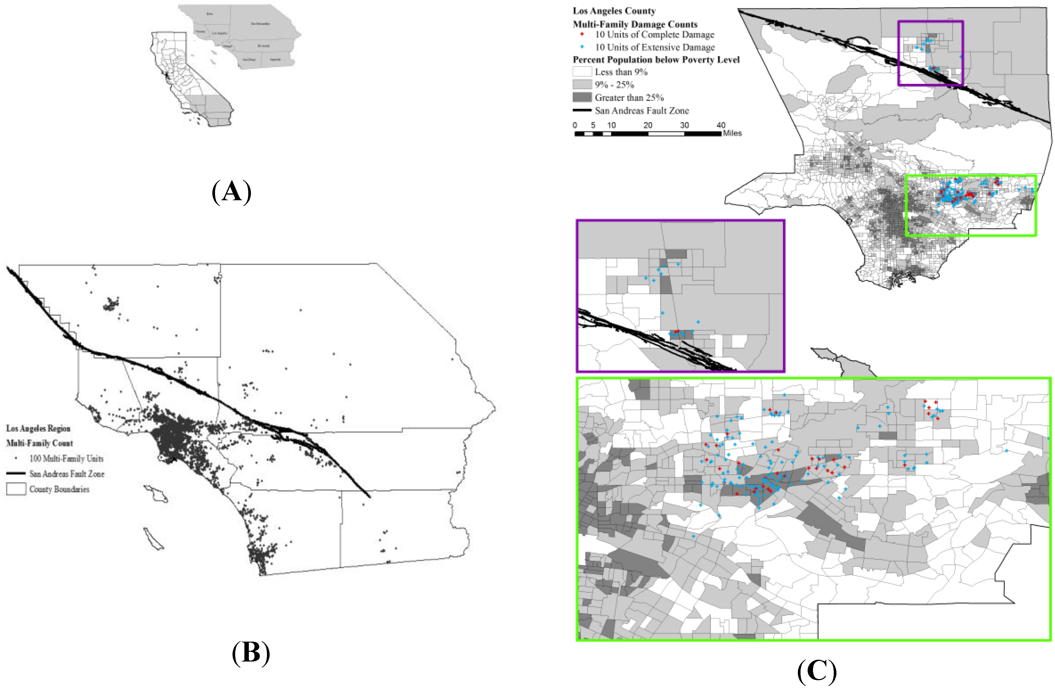
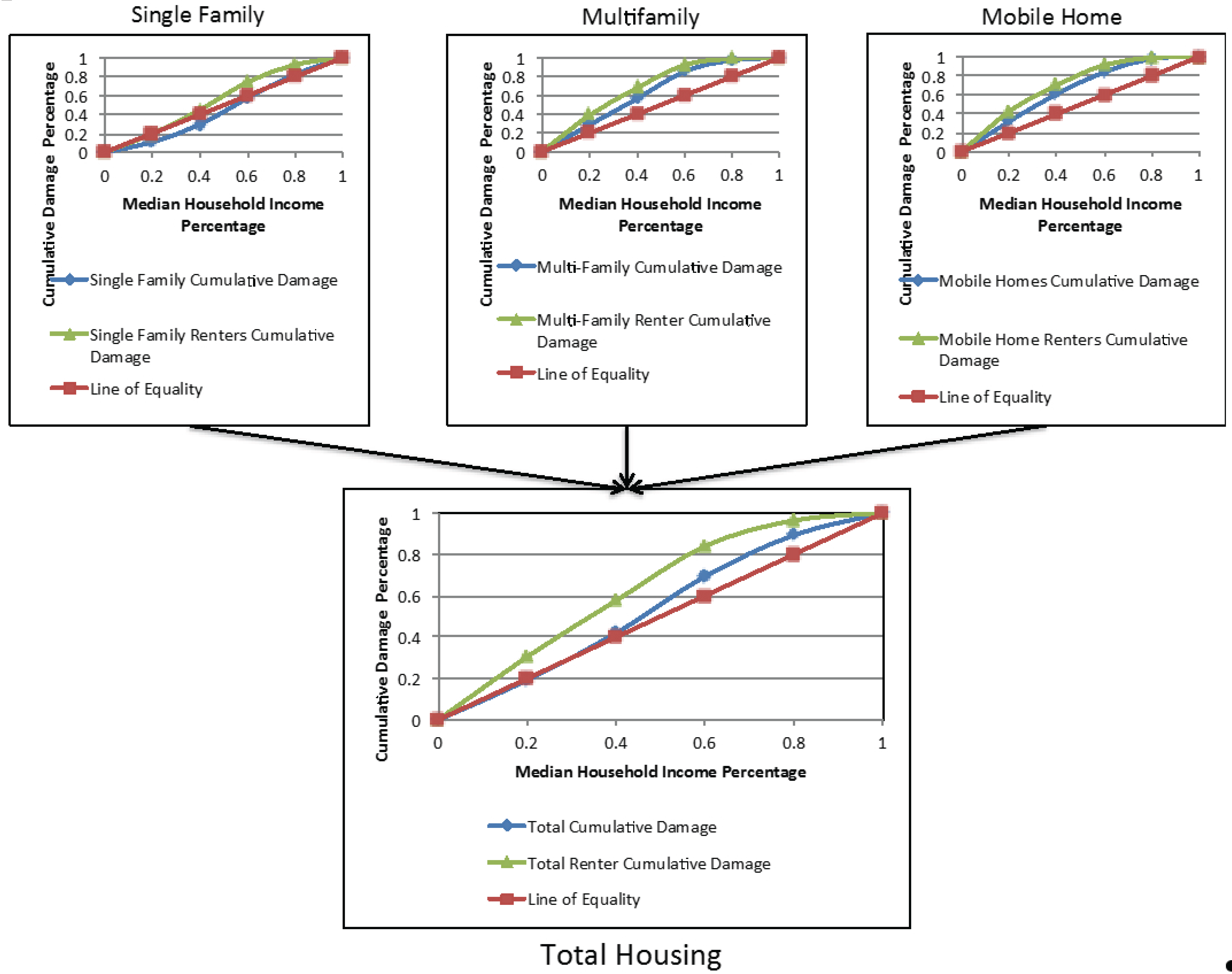
4. Example 2. An Inductive Prospective Model—An Application to Earthquake Hazards Mitigation and Income Distribution: Geospatial Information Provides Input for Earthquake Housing Risk Concentration in a Hazard Scenario for a Hazard Scenario

This example is a prospective model for assessing the economic benefits of geospatial information in a natural hazard scenario to evaluate housing mitigation policy and planning. In 2008 the United States Geological Survey (USGS) published the ShakeOut hazard scenario for a great earthquake and its impacts on southern California [22]. The southern California study area included Imperial, Kern, Los Angeles, Orange, Riverside, San Bernardino, San Diego, and Ventura counties. The regional hazard scenario provided a “state of the art” simulation of a possible Magnitude 7.8 earthquake along the southernmost segment of the San Andreas Fault in CA. The hazard scenario was an application of available earthquake research information including: trenching and evidence of prehistoric earthquakes, instrumental recordings of large earthquakes, and the latest theory in earthquake source physics [22]. The USGS ShakeOut scenario, although not an actual disaster, had results that were consistent with the housing outcomes in previous events [23]. The VOI analysis seeks to quantify the extent to which earthquake damages could be reduced if local ordinances considered detailed geospatial information, such as that resulting from the simulation of a potential earthquake disaster. The baseline in this example is to rely on past damage estimates from earthquakes or other hazardous events and building specific building failure simulations derived from hypothetical earthquakes.

4.1. Background

Studies of the Loma Prieta and Northridge California earthquakes and Hurricane Katrina documented that housing recovery depends on: the geographic concentration of housing damage (which depends on the distribution of different types of housing structures, i.e., single-family, multi-family, and mobile homes), and the socioeconomic status of people in the affected areas [23].

Natural scientists develop hazard scenarios for stakeholders and emergency officials to assess the impacts of a particular disaster outcome. In contrast, social scientists can use the geospatial information to identify and alert decision makers to the socioeconomic impacts of the disaster. Furthermore, social scientists have found that housing losses and recovery affect individuals in lower socioeconomic status disproportionately. For example, the USGS ShakeOut scenario residential building losses amounted to $16.7 billion for eight counties in southern California (see Figure 6A for a map of the example). By classifying residential housing into single-family, multi-family, and mobile homes it is possible to represent the concentration of damage for each occupancy category by socioeconomic status compiled by census tract.

Figure 6. (A) Map of the USGS ShakeOut scenario region. (B) Map of the distribution of 100 multi-family units. (C) Map by census tract and poverty class of at least 10 multi-family housing units in the extensive and complete damages categories Los Angeles County (source: [24]).

Figure 6. (A) Map of the USGS ShakeOut scenario region. (B) Map of the distribution of 100 multi-family units. (C) Map by census tract and poverty class of at least 10 multi-family housing units in the extensive and complete damages categories Los Angeles County (source: [24]).

Societal conditions are an important factor in determining housing vulnerability. Housing vulnerability is estimated using the set of characteristics that a community has selected that identify buildings that could be affected by an earthquake that lead to damage costs. People and households in poverty are likely to live in poorly built and inadequately maintained housing. They are the least prepared for an earthquake, making them more vulnerable to disastrous outcomes such as loss of life and property and forced migration [25,26]. From a community perspective, low-income people are likely to need substantial assistance during response and recovery because large numbers of them will be homeless and require temporary housing [26].

4.2. Analysis

In this example the modeling approach considers both regional economic output and natural disaster policy decisions that uses geospatial socioeconomic and natural hazard information. Trade-offs occur between economic development and safety and loss avoidance. The ShakeOut scenario provides a conditional probability of ground failure. That information combined with a building inventory produce a spatially explicit damage estimate [22]. The detailed map of expected loss shows locations where regional economic output would be negatively affected. This impact would be especially problematic, in terms of recovery, in densely populated, low-income areas. To avoid or reduce the impact of the disaster in these areas, more resilient buildings could yield less downtime for economic production (for both labor and equipment) and also less financial aid required for recovery.

The regional economy is assumed to be in equilibrium and the economy is at a location on PPF₀ (the graph in Figure A1 illustrates this example). However the amount spent on structural (housing) mitigation would require resources that could reduce regional economic output. This is shown as a tradeoff along the PPF frontier. The baseline PPF₀ represents the regional output and level of housing resilience, without the geospatial information derived from the ShakeOut scenario (see Figure A1). With the information from the scenario, more detailed targeting of expected damage is possible, and a science based hazard assessment can be used to achieve more cost effective mitigation; hence a shift to a new possible production, PPF₁. The VOI of the geospatial information can be calculated as the shift in regional economic output from the PPF₀ line to the PPF₁ line. Figure 6A shows two starting points for a shift: (1) point A, an economy that produces greater output with less resources spent on building resilience, and (2) point B, an economy with less output but greater investment in building resilience. The additional geospatial information may allow better targeting of policies and local ordinances to maintain or improve regional production while also increasing the number of resilient housing units.

The conditional distribution of damage cost (determined in the USGS ShakeOut earthquake scenario) was translated into a measure to prioritize investment decisions for earthquake hazard mitigation. A specific application of the scenario produced geospatial information that identified greater potential risk (i.e., damage costs) in census tracts with greater numbers of people with lower incomes. This can be seen for multi-family units in the region in Figure 6B and the locations of severe damage to multi-family units for the county in Figure 6C. The enlarged areas in Figure 6C locate clusters of extensive and complete damage in census tracts with large populations of lower income residents including many below the poverty line (gray census tracts). These census tracts have similar attributes to areas where recoveries were hampered in previous earthquakes or following Hurricane Katrina [27,28,29]. Landscape inequality, which includes the human dimension, caused by a natural hazard is a significant risk to a region’s capacity to recover from a disaster. Geospatial information can contribute to reducing the landscape inequality by translating the scenario outcome to a decision framework for estimating the economic impact on specific income groups (The framework contains a set of consequences or outcomes that provides a process for making decisions.). To accomplish this objective the geospatial information was used to construct a regional concentration curve and index.

The regional concentration curve is a plot of the cumulative percentage of simulated damage of a disaster against the cumulative percentage of the income of the regional population, ranked from lowest to highest incomes [30]. Figure 7 contains regional concentration curves for each housing type and for total housing. If damage is distributed equally across all income groups, the concentration curve is a 45-degree line or line of equality (red line in Figure 7). When the hazard damage variable has higher values among lower income groups, the concentration curve lies above the line of equality (blue line for owners and green line for renters). The farther the concentration curve is above the equality line, the greater the density of the losses in lower income groups. On the other hand, if the damage variable has higher values among higher income groups, the concentration curve lies below the line of equality. Also, the farther the curve is below the line of equality there is greater density of losses in higher income groups.

Figure 7. Earthquake risk concentration curve of cumulative damage ranked by median household income (source: [24]).

Figure 7. Earthquake risk concentration curve of cumulative damage ranked by median household income (source: [24]).

Except for the total single-family housing line that crosses the line of equality, both total housing and renter concentration fall above the line of equality meaning there is a concentration of extensive and complete damage in lower income groups. The same is true for renters of single-family housing units.

The regional concentration index and curve is a component of a spatial Gini index as a measure of income distribution that represents a natural hazard risk [31]. The regional concentration index provides a statistically robust estimate of the physical impacts of the hazard and the socioeconomic status across income groups in the regional population [30,32]. Using the scenario, the index for single-family housing units exhibits a small positive sign and is statistically significant at the p = 0.008 level. This inference reflects a concentration of risk in higher income groups [24]. On the other hand, multi-family buildings and mobile home units are associated with large negative concentration indexes and are statistically significant at p < 0.001. This means a strong concentration in lower income groups. In the example our modeling approach was to devise a county level building retrofit policy focused on multi-family buildings.

In the scenario, 26% of the square footage of inventoried multi-family buildings would be subject to MMI VIII-IX shaking and therefore, could suffer an estimated $2.9B of severe and total building loss [22]. The ShakeOut Scenario included Modified Mercalli Intensity (MMI). MMI is a way to assess damage that is familiar to the engineering and emergency management communities. Buildings in locations of MMI > VII shaking are at greatest risk [22]. To estimate damages to structures in the ShakeOut Scenario ground motion parameters were calculated. Ground motion parameters describe how the ground moves due to different measures of earthquake waves, and are needed because different kinds of structures are damaged by different kinds of waves. Los Angeles County was chosen for the example net benefits analysis because approximately 42.2% of the county population resided in multi-unit structures in 2000 (United States Census Bureau, 2000). There were 2183 multi-family buildings that suffered extensive and complete damage in the scenario, of which 1601 buildings were located in census tracts with at least 10 units suffering extensive and complete damage (clusters) and 582 buildings in census tracts without damage clusters. Census tracts with clustered damages outnumbered non-clustered damages by 2.75:1 while only 4.2% (87 of 2054) of all census tracts in the county were identified to have at least ten buildings with extensive and complete damage [24].

Adopting a regulatory policy for retrofitting existing buildings [33] is one way to reduce the societal cost of an earthquake. Current retrofit mitigation is voluntary: investments are based on individual owner decisions either and relate to occupant safety and/or to the assessments of expected damage costs relative to protection costs. Voluntary mitigation assumes that all building owners have sufficient resources to purchase earthquake insurance and/or to invest in mitigation to enhance structure and community resiliency. The expected net benefit of voluntary mitigation must be positive.

Alternatively, government could incentivize or mandate building retrofit by identifying the housing hazard exposure for the largest number of people at the greatest risk. This approach could combine the expected net benefits of mitigation and public investment with the targeting of areas of highest risk. The approach is referred to as a cost minimizing regulation. Housing mitigation is based on the building owner receiving public economic incentives, in qualified areas, to conduct a retrofit. There are four steps used to determine incentive eligibility:

(1)

Apply hazard scenario to indicate the presence and significance of risk concentration by type of housing as a threshold for public sector intervention. If the risk concentration index is negative, this means there is a risk concentration for lower income groups for a given housing type.

(2)

Identify census tracts with damage clusters of at least 10 extensive and complete damaged multi-family buildings from the scenario. The threshold for the number of buildings at 10 was chosen as a reasonable approximation to what would be considered a significant impact to closely spaced structures in a census tract in an urban area [24].

(3)

Intersect damage clusters with a poverty threshold by census tract.

(4)

Estimate the net benefit of regulatory mitigation and compare the results of expected outcomes with voluntary mitigation for census tracts identified in steps (1)–(3). If the four criteria are met, the cost minimizing regulation program could be made available for all multi-family buildings in a census tract to avoid any missed special circumstances.

4.3. Results

The results of the Los Angeles County application for the voluntary program had net benefits of about $1.1B if mitigation costs are approximately 10% of exposed multi-family real estate value. If mitigation costs are higher, say up to 50% of value, net benefits fall to below $0.4B. For the analysis, mitigation cost is estimated as a sliding scale of the percent of exposed value and allowed to vary by building type, quality, age, location, and loss-reduction measure (design and level of protection). The application of the cost minimizing regulation had net benefits that varied from $0.5B to $0.1B depending on the mitigation costs. There were 2054 (2.6%) census tracts in the county that met the income criterion for the cost minimizing regulation program, where at least 9% of the population is below the poverty line (cf. light gray census tracts in Figure 6C). There were 17 of those 2054 (0.8%) census tracts additionally that met criteria for the program, where at least 25% of the population is below the poverty line (cf. dark gray census tracts in Figure 6C). An interesting case is when the policies are both in effect. The example showed that a combined program of both policies increases the net benefits relative to voluntary mitigation. In this case, the county and its citizens are economically better off if the mitigation costs per tract rise above 16%. For implementation, the county would apply the voluntary program until mitigation costs cross the threshold, then at costs above the threshold, application of the cost minimizing regulation program offers additional net benefits. That is, as mitigation cost rises beyond 16% the combined program translates into $59M additional net benefits and 163 more buildings that would not have been mitigated under the voluntary mitigation policy.

4.4. Summary

Policy decisions involving investments in loss reduction measures and response and recovery are best informed by the integration of geospatial data with scientific and socioeconomic information. The scenario produced a geographic pattern of risk concentration based on the colocation of earthquake shaking, specific housing types and lower income groups in an urban region [24]. The pattern that emerged was that a greater level of severe damage to multi-family buildings and mobile homes would be concentrated in high density, low-income census tracts in an 8-county area in the Los Angeles region. The simulated damage pattern is consistent with recent natural disasters in the US.

One of the values of the geospatial information in a hazard scenario is to assess the efficiency and equity of public policy decisions. The combination of the hazard scenario and the concentration curve and index can be part of a spatially explicit approach to estimating the socioeconomic benefits and costs of investing in regional scale mitigation. The policy question was whether public sector investment in mitigation should be undertaken in locations where building and income vulnerability are concentrated. The VOI of the geospatial analysis derives from the fact that, with limited resources, decision makers need a way to prioritize mitigation investments. Income distribution when coupled with the hazard scenario depicted a geographic pattern of what could happen to vulnerable populations. By targeting disadvantaged populations a retrofit building code for multi-family buildings could identify where public intervention and investment would be cost effective.

The public program benefits rise as the cost of mitigation increases with the level of protection. Hence the VOI of the geospatial information for a publicly financed mitigation program would focus on neighborhoods containing populations in lower socioeconomic quintiles. The program would become more valuable as the cost of mitigation became a greater percent of replacement value. The expected payoff of this policy would increase landscape equality by reducing disaster losses, shortening recovery times, and avoiding excessive recovery costs. A more equal distribution of damage could be achieved by targeting mitigation in areas that could suffer the greatest impact. The socioeconomic benefit of the geospatial information is the support the data provides for policy development.

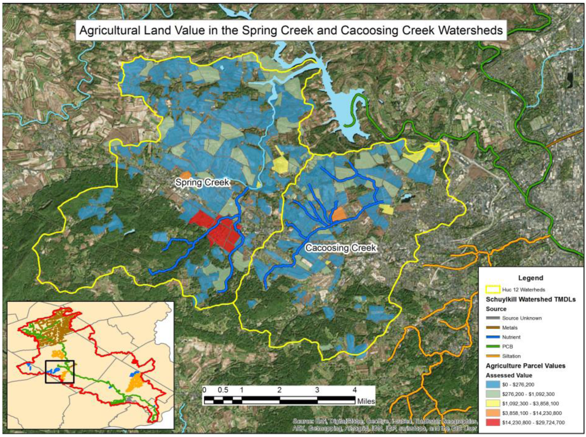
5. Example 3: A Private—Public Integrated Market Model for Ecosystem Services Markets. An Application of Geospatial Information can Provide an Objective, Replicable Accounting Framework to Reduce Transactions Costs in Environmental Market(s) Activities

This example is a prospective model about the use of remote sensing in ecosystem services markets to reduce environmental externalities. The content, quality and scale of geospatial information can help cap and trade markets to function more efficiently. Both “general” (public good) and “specific” (private good) geospatial remote sensing information is a way to frequently monitor creditable assets involved in reducing environmental externalities. The VOI issue is whether market transaction costs can be reduced because remotely sensed data can provide an improvement in monitoring and enforcement of market crediting and verification responsibilities; and lower market administration costs. The example is currently in development and examination [34]. The approach is to assess the veracity of a multi-scale, multispectral approach to an ecosystem services market oriented program based on MRLI and high-resolution imagery to lower market costs. The baseline in this example is to rely on periodic updating of water quality stream measurements at current locations and regulatory data collected for U.S. EPA total daily maximum load regulations at specific locations along a river or other water body.

5.1. Background

An ecosystem market is a system where the attributes or ecosystem services of an ecosystem are exchanged [35]. Ecosystem services, as listed by the 2003 Millennium Ecosystem Assessment, range from the provision of fresh water to nutrient cycling. An ecosystem cap and trade market aims to increase the quality and quantity of ecosystem services such as habitat preservation, habitat rejuvenation, and species preservation. Current externality markets utilize credit systems to represent the “attribute” that is being traded. These credits can represent a quantity, such as a pound of pollution or amount of conservation to preserve or restore river water quality, as seen in mitigation markets. Ecosystem (or externality) markets assume that there is an optimal value of ecosystem cleanliness. The markets aim to efficiently allocate the societal cost of environmental externalities that are not always taken into account by those causing degradation to the ecosystem attributes. The attempt is to reach an efficient allocation of pollution, conservation, or ecosystem preservation.

In a cap-and-trade style market the total quantity of emissions is decided upon and then credits are allocated to emitting firms. A firm receiving emissions credits may emit pollution up to the permit amount, or may reduce emissions and sell the permit to pollute in the market [35]. Water quality and pollution trading markets and partnerships have been created across river basins in an effort to reduce pollution. As an example, the Willamette River has been using a cap and trade permit system since 2005 [36]. This system creates an incentive based program to reduce the pollution load of the river. The Willamette River Partnership used the US EPA’s recommended total maximum daily load (TMDL) limits and used them towards creating a cap and trade system of permits to reduce thermal and bacterial pollution [36]. This type of market minimizes total cost of pollution abatement by incentivizing each individual producer to minimize costs.

Although creating a market for ecosystem services is not a novel concept, the application of remote sensing in a market approach for reducing pollution and sustaining ecosystem services is. The Willamette Partnership [37] identified a need for frequent monitoring of all the creditable assets involved in reducing environmental externalities for a market to function efficiently.

5.2. Analysis

Both panchromatic and spectral imagery at multiple resolutions as well as other geospatial information can be used to track and monitor changes in land use and land cover, identify emission sources and monitor those sources such as reduced loading of impaired streams at sub-watershed resolution (i.e., to track changes in effluent quantities). A recent decision by the US Department of Commerce permitted the commercial sale of high-resolution earth observations. This in turn allows improved monitoring and analysis of a market portfolio of ecosystem services that require detailed, replicable geospatial data [38]. The geospatial imagery can be used to verify quantities and any “attribute” changes for credit monitoring. For example midlevel (30 m–250 m resolution panchromatic and spectral bands) and detailed (0.3 m resolution panchromatic and 1.4 m spectral bands) land imagery can be used in a hierarchical system to monitor changes in agricultural practices to reduce nitrogen loading of streams. Figure 8 is an example in the Schuylkill Watershed in eastern PA. MRLI and high-resolution imagery can assist the market by identifying changes to registered land parcels and thereby validating, or invalidating crediting activities.

The application of remote sensing could be a critical component for the market as part of the administration and enforcement and consequential penalty aspects of an ecosystem service(s) marketplace. The geospatial information is objective and replicable for any disputes, and entails a lower cost than a market operation without the information. The information can be used to lower transactions costs, which would improve market efficiency, and may reduce cheating because landowners would be aware they are being observed. The activity could increase social welfare. In addition the geospatial information introduces a way to monitor spatiotemporal risks and their effects on return. This is easily seen in Figure 9. The ecological values of specific parcels could be located to take advantage of land characteristics and economies of scale that promote converting current agricultural land to forest by targeting locations with specific characteristics.

Figure 8. Map of land use, sub-watersheds, property values and impaired waterways.

Figure 8. Map of land use, sub-watersheds, property values and impaired waterways.

Figure 9. An ecosystem services market with land-use offsets that uses remote sensing monitoring.

Figure 9. An ecosystem services market with land-use offsets that uses remote sensing monitoring.

5.3. Summary

Again, as in the earlier examples, the geospatial data and archives establish a baseline. In this case, the spatiotemporal observations can be used to account for certain types of ecosystem services by identifying changes to a land portfolio and verifying market credit. Geospatial data can help administer and plan the market over time by showing preferred parcels to maximize the societal benefits of pollution reduction (source: [34]).

In addition to helping quantify ecosystem services, remote sensing may allow us to create new kinds of market credits. Having the archival data to evaluate risks and changes over time provides the market with periodic updates about the ecosystem services, which makes the market somewhat more “investor-friendly” for buyers.

6. Conclusions

The benefits to society of geospatial information result from the use of the information in decision making. It is critical that we improve our understanding of these benefits because we will always have imperfect information and uncertainty. Improving our understanding of the benefits from alternative portfolios of information can help us prioritize future investments in information so that scarce resources are used most effectively. We have presented an economic approach to identify and develop specific applications of geospatial information and to estimate the potential benefits of the information. The examples presented show improvements in economic efficiency in benefit-cost frameworks, as a result of investments in geospatial monitoring and analysis. The premise is that an empirical economic model is the way to approach the VOI problem. The approach outlined demonstrates the benefits of supplying geospatial data that enhances productivity and promotes economic growth. The three examples described offer specific cases that can provide significant benefits for environmental regulation, natural hazard mitigation and support for ecosystems services cap and trade markets.

Advances in technology, such as high-resolution earth observation that can be considered “specific” information, have added new potential inputs to decision making. Although the benefits for specific use cases of geospatial information would be substantial, implementation is not obvious or simple. Barriers to use exist because applications will require investment in integrated models. Open access to the data does not necessarily provide open access to the application or interpretation of the data.

References

- Oxford Reference. Available online: http://0-www-oxfordreference-com.brum.beds.ac.uk/view/10.1093/oi/authority.20110803100023635 (accessed on 1 September 2014).
- Forney, W.; Raunikar, R.; Bernknopf, R.; Mishra, S. An Economic Value of Remote-Sensing Information—Application to Agricultural Production and Maintaining Groundwater Quality; U.S. Geological Survey: Reston, VA, USA, 2012.
- Schimmelphennig, D.; Norton, G. What is the value of agricultural economics research? Am. J. Agric. Econ. 2003, 85, 81–94. [Google Scholar] [CrossRef]
- Bemknopf, R.; Dinitz, L.; Loague, K. An Interdisciplinary Assessment of Regional-Scale Nonpoint Ground-Water Vulnerability: Theory and Application; U.S. Geological Survey: Reston, VA, USA, 2001.
- Bradford, D.; Kelegian, H. The value of information for crop forecasting in a market system: Some theoretical issues. Rev. Econ. Stud. 1997, 44, 519–531. [Google Scholar] [CrossRef]
- Bernknopf, R.; Wein, A.; Lucas, S.M.; St-Onge, M. Analysis of Improved Government Geological Map Information to Mineral Exploration: Incorporating Efficiency, Effectiveness and Risk Considerations; Geological Survey of Canada Bulletin 593; U.S. Geological Survey: Reston, VA, USA, 2007.
- Bernknopf, R.L.; Brookshire, D.S.; Soller, D.R.; McKee, M.J.; Sutter, J.C.; Matti, J.; Campbell, R.H. The Societal Value of Geologic Maps; United States Government Publishing Office: Washington, DC, USA, 1993.
- Khabarov, N.; Moltchanova, E.; Obersteiner, M. Valuing weather observation systems for forest fire management. IEEE Syst. J. 2008, 2, 349–357. [Google Scholar] [CrossRef]
- Kite-Powell, H. The value of ocean surface wind information for maritime commerce. Mar. Technol. Soc. J. 2011, 45, 75–84. [Google Scholar] [CrossRef]
- Fox, P. The Role of Virtual Observatories and Data Frameworks in an Era of Big Data. Available online: http://www.nist.gov/itl/ssd/is/big-data.cfm (accessed on 01 September 2014).
- Windrum, P.; Fagiolo, G.; Moneta, A. Empirical Validation of Agent-Based Models: Alternatives and Prospects. Available online: http://jasss.soc.surrey.ac.uk/10/2/8.html (accessed 05 April 2014).
- Wikipedia—Big Data. Available online: http://en.wikipedia.org/wiki/Big_data (accessed on 25 August 2014).
- Halsing, D.; Theissen, K.; Bernknopf, R. A Cost-Benefit Analysis of the National Map; U.S. Geological Survey: Reston, VA, USA, 2004.
- Varian, H. Intermediate Microeconomics: A Modern Approach, 6th ed.; W.W. Norton & Company: New York, NY, USA, 2003. [Google Scholar]
- What is an Inductive Method in Economics? Available online: http://sundaramponnusamy.hubpages.com/hub/What-is-an-Inductive-Method-in-Economics (accessed on 10 August 2014).
- Bernknopf, R.; Forney, W.; Raunikar, R.; Mishra, S. A general framework for estimating the benefits of moderate resolution land imagery in environmental applications. In Value of Information: Methodological Frontiers and New Applications; Laxminarayan, R., Macauley, M., Eds.; Springer Publishers: Berlin, Germany, 2012; pp. 257–300. [Google Scholar]
- Ceric, A.; Haitjema, H. On using simple time-of travel capture zone delineation methods. Ground Water 2005, 43, 408–412. [Google Scholar] [CrossRef] [PubMed]
- Yadav, S. Dynamic optimization of nitrogen use when groundwater contamination is internalized at the standard in the long run. Am. J. Agric. Econ. 1997, 79, 931–945. [Google Scholar] [CrossRef]
- Kim, C.; Hostetler, J.; Amacher, G. The regulation of groundwater quality with delayed responses. Water Resour. Res. 1993, 29, 1369–1377. [Google Scholar] [CrossRef]
- The University of Reading ECIFM Monoculture. Available online: http://www.ecifm.rdg.ac.uk/monoculture.htm (accessed on 17 July 2014).
- Raunikar, R.P.; Forney, W.M.; Benjamin, S.P. What is the Economic Value of Satellite Imagery? USGS Fact Sheet 2013–3003; U.S. Geological Survey: Reston, VA, USA, 2013.
- Jones, L.; Bernknopf, R.; Cox, D.; Goltz, J.; Hudnut, K.; Mileti, D.; Perry, S.; Ponti, D.; Porter, K.; Reichle, M.; et al. The ShakeOut Scenario; USGS Open File Report 2008–1150; USGS: Reston, VA, USA.
- Wein, A.; Johnson, L.; Bernknopf, R. Recovering from the shakeout earthquake. Earthq. Spectra 2011, 27, 521–538. [Google Scholar] [CrossRef]
- Bernknopf, R.; Amos, P. Measuring earthquake risk concentration for hazard mitigation. Natural Hazards 2014, 74, 2163–2192. [Google Scholar] [CrossRef]
- Zahran, S.; Brody, S.; Peacock, W.; Vedlitz, A.; Grover, H. Social vulnerability and the natural and built environment: A model of flood casualties in Texas. Disasters 2008, 32, 517–560. [Google Scholar] [CrossRef] [PubMed]
- Kunreuther, H.; Platt, R.; Baruch, S.; Bernknopf, R.; Buckley, M.; Burkett, V.; Conrad, D.; Davison, T.; Deutsch, K.; Geis, D.; et al. The Hidden Cost of Coastal Hazards: Implications for Risk Assessment and Mitigation; Island Press: Washington, DC, USA, 1999. [Google Scholar]
- Vigdor, J. The economic aftermath of Hurricane Katrina. J. Econ. Perspect. 2008, 22, 135–154. [Google Scholar] [CrossRef]
- Masozera, M.; Bailey, M.; Kerchner, C. Distribution of impacts of natural disasters across income groups: A case study of New Orleans. Ecol. Econ. 2007, 63, 299–306. [Google Scholar] [CrossRef]
- Comerio, M.C. Housing Repair and Reconstruction after Loma Prieta. Available online: http://nisee.berkeley.edu/loma_prieta/comerio.html (accessed on 23 June 2010).
- O’Donnell, O.; van Doorslaer, E.; Wagstaff, A.; Lindelow, M. Analyzing Health Equity Using Household Survey Data: A Guide to Techniques and Their Implementation. Available online: http://siteresources.worldbank.org/INTPAH/resources/Publications/459843-1195594469249/HealthEquityFINAL.pdf (accessed on 15 September 2011).
- Kakwani, N. Income Inequality, Welfare, and Poverty: An Illustration using Ukrainian Data. Available online: http://ssrn.com/abstract=623915 (accessed on 1 October 2011).
- Kakwani, N.; Wagstaff, A.; van Doorslaer, E. Socioeconomic inequalities in health: Measurement, computation, and statistical inference. J. Econ. 1997, 77, 87–103. [Google Scholar] [CrossRef]
- Feinstein, D. To Provide Incentives to Encourage Private Sector Efforts to Reduce Earthquake Losses, to Establish a National Disaster Mitigation Program, and for Other Purposes; U.S. Government Printing Office: Washington, DC, USA, 2001.
- Zhang, E.; Bernknopf, R.; Amos, P. Generation of a multi-permit model for ecosystem services using the portfolio approach. University of Pennsylvania: Philadelphia, PA, USA, Unpublished work; 2015. [Google Scholar]
- Bridge, B.; Brookshire, D.; Broadbent, C.; Bernknopf, R.; Pesko, S. Conceptual framework and market for nitrate loading in the Tensas river basin. University of New Mexico: Albuquerque, NM, USA, Unpublished work; 2015. [Google Scholar]
- Pacific Northwest Agencies and Partners Announce Recommendations for Regional Water Quality Trading. Available online: http://www.thefreshwatertrust.org/press-release-8132014/ (accessed on 21 September 2014).
- Willamette River TMDL East and West TMDL Alternatives Due Diligence Evaluation. Available online: http://www.corvallisoregon.gov/modules/showdocument.aspx?documentid=6360 (accessed on 20 August 2014).
- WorldView-3 Satellite Images. Available online: http://www.satimagingcorp.com/gallery/worldview-3/ (accessed 22 September 2014).
© 2015 by the authors; licensee MDPI, Basel, Switzerland. This article is an open access article distributed under the terms and conditions of the Creative Commons Attribution license (http://creativecommons.org/licenses/by/4.0/).
Share and Cite
Bernknopf, R.; Shapiro, C. Economic Assessment of the Use Value of Geospatial Information. ISPRS Int. J. Geo-Inf. 2015, 4, 1142-1165. https://0-doi-org.brum.beds.ac.uk/10.3390/ijgi4031142
Bernknopf R, Shapiro C. Economic Assessment of the Use Value of Geospatial Information. ISPRS International Journal of Geo-Information. 2015; 4(3):1142-1165. https://0-doi-org.brum.beds.ac.uk/10.3390/ijgi4031142
Chicago/Turabian StyleBernknopf, Richard, and Carl Shapiro. 2015. "Economic Assessment of the Use Value of Geospatial Information" ISPRS International Journal of Geo-Information 4, no. 3: 1142-1165. https://0-doi-org.brum.beds.ac.uk/10.3390/ijgi4031142