
A Progressive Buffering Method for Road Map Update Using OpenStreetMap Data


Abstract
:1. Introduction
2. Methodology
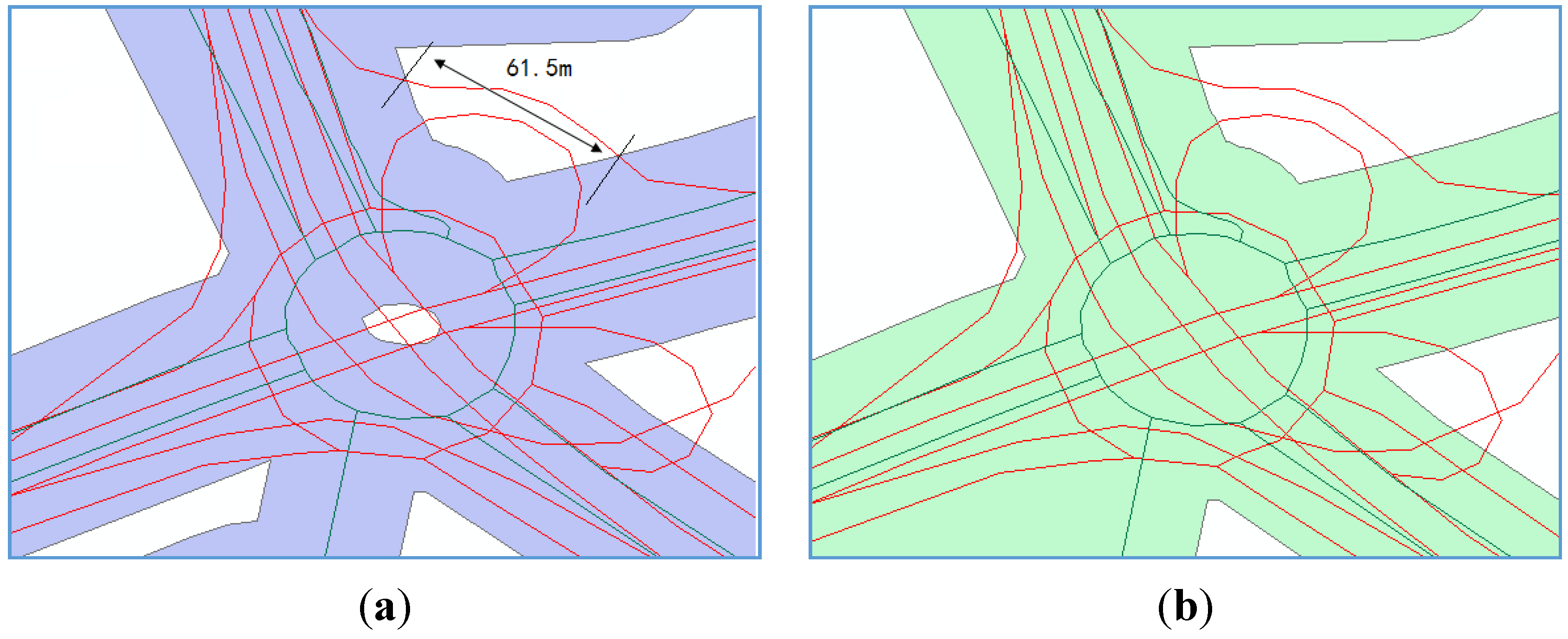
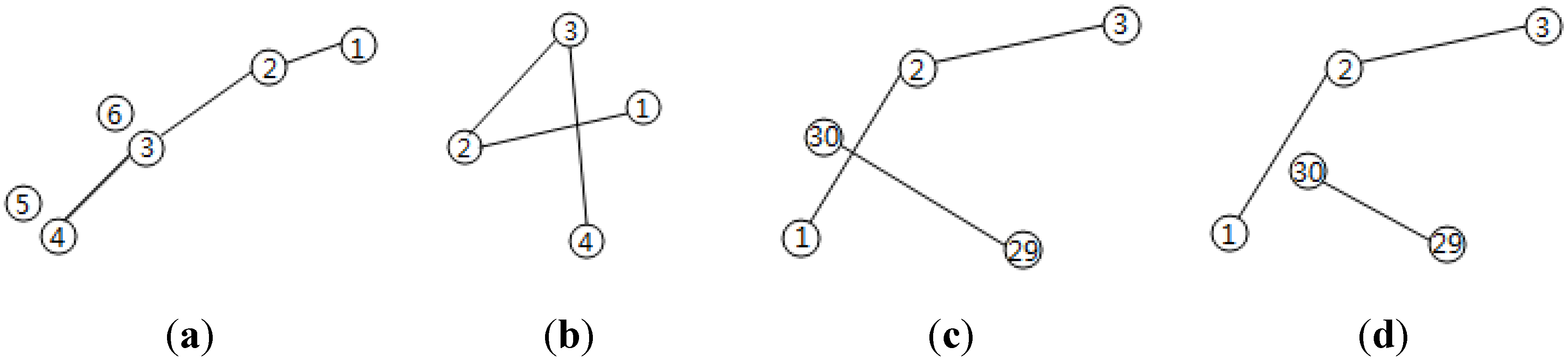
2.1. Buffer and Intersect Analysis


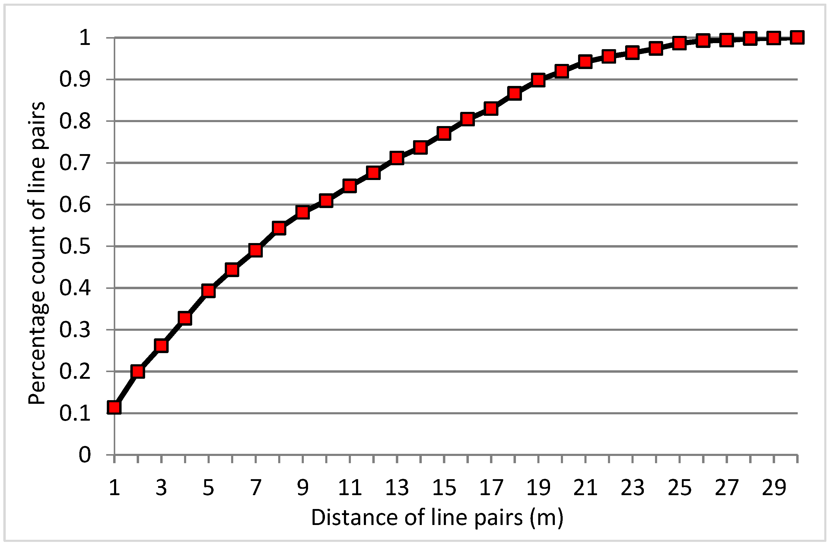
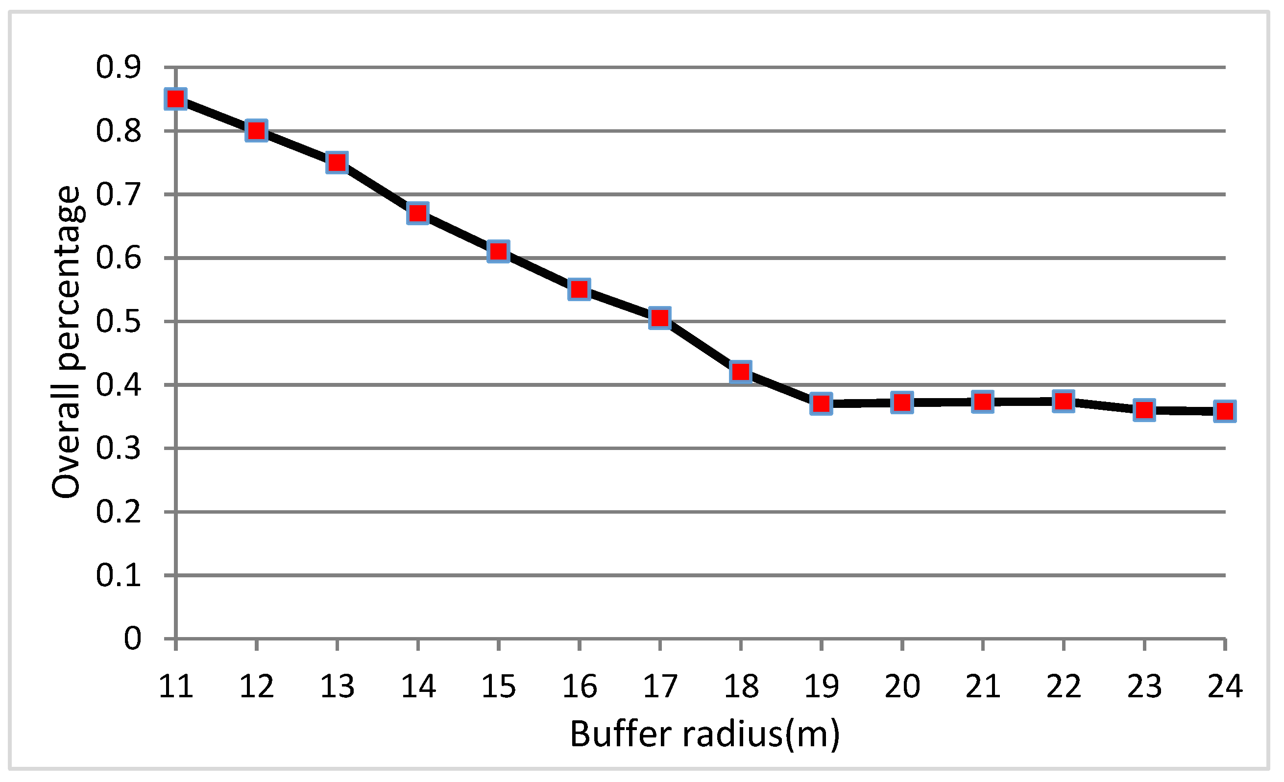
2.2. Progressive Buffering


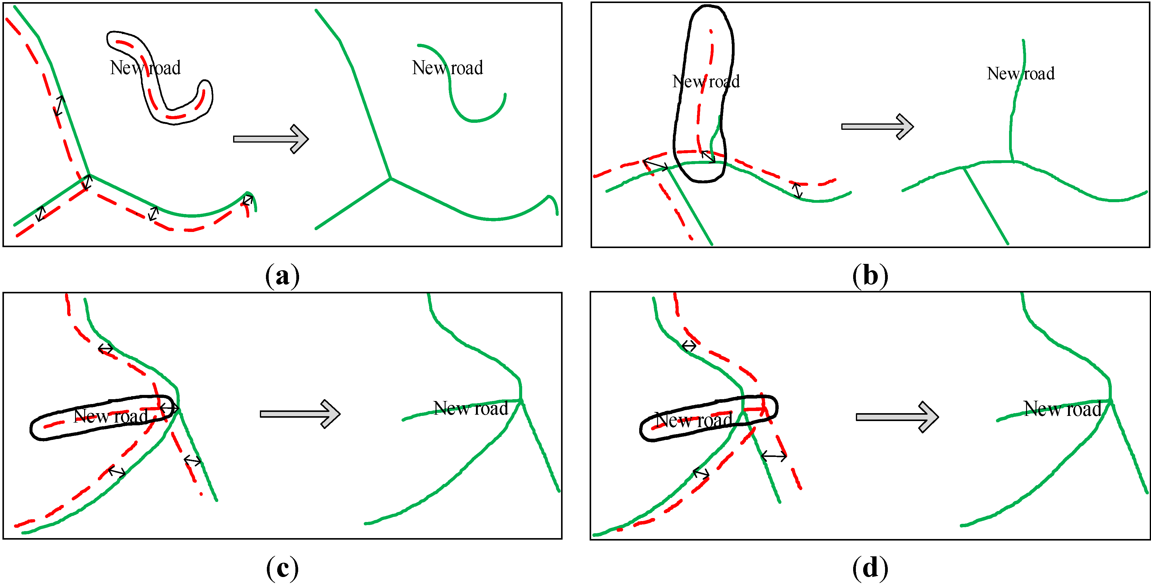
2.3. Add New Roads to the Reference Roads


| OSM | Ying | Yuan | Road | ||
|---|---|---|---|---|---|
| Reference | |||||
| 0 | 1 | 2 | 3 | ||
| Da | 1 | 1 | 2 | 3 | |
| Xue | 2 | 2 | 2 | 3 | |
| Yuan | 3 | 3 | 2 | 3 | |
| Road | 4 | 4 | 3 | 2 | |
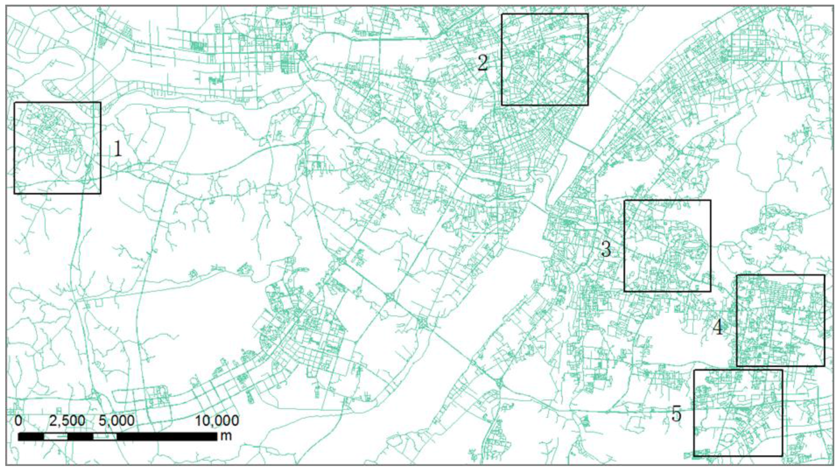
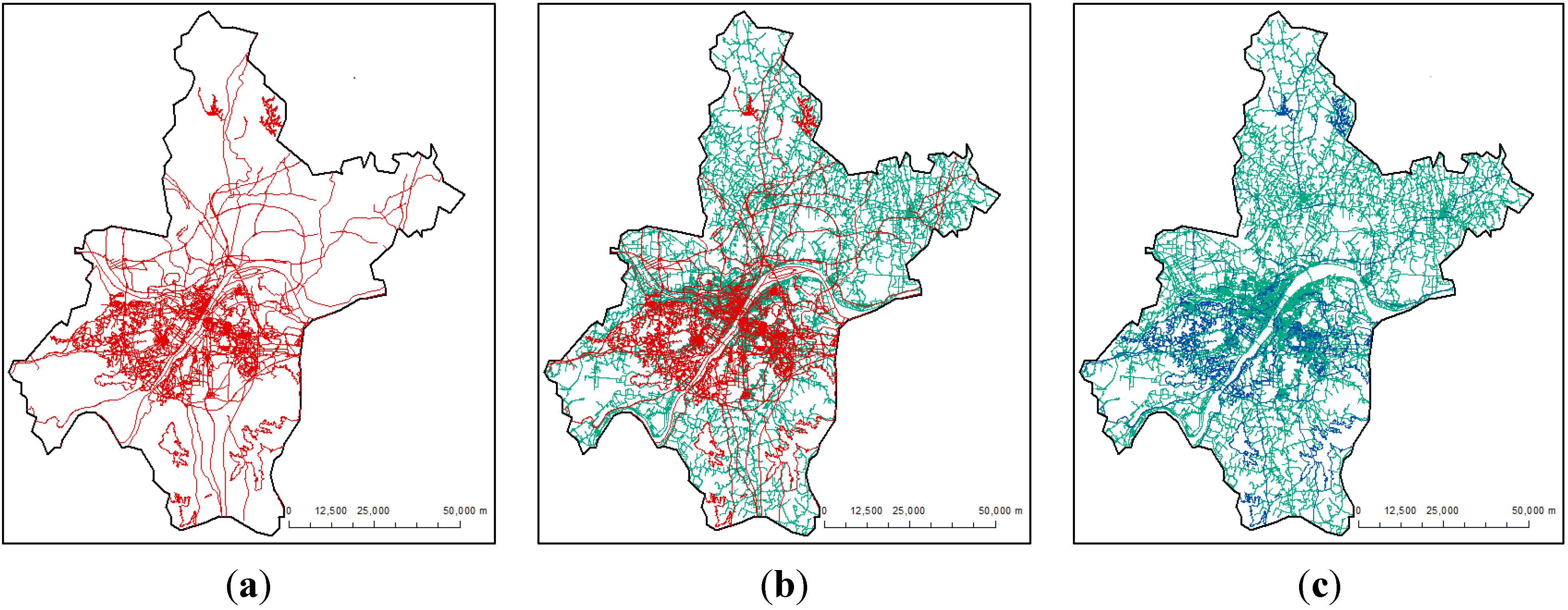
3. Test Data


| Redundancy | Self-Intersection | Over-Shoot | Under-Shoot | Total |
|---|---|---|---|---|
| 86 | 47 | 56 | 72 | 261 |
4. Results and Discussion
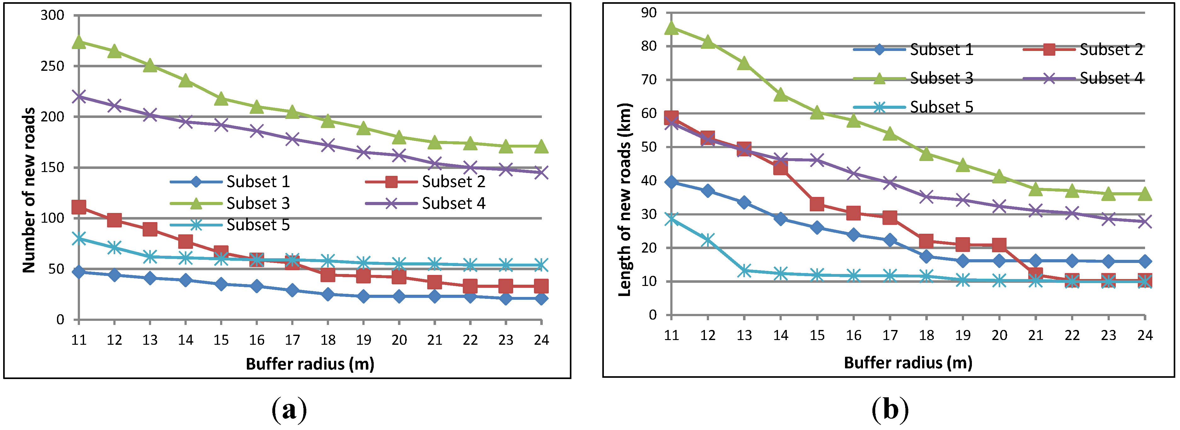
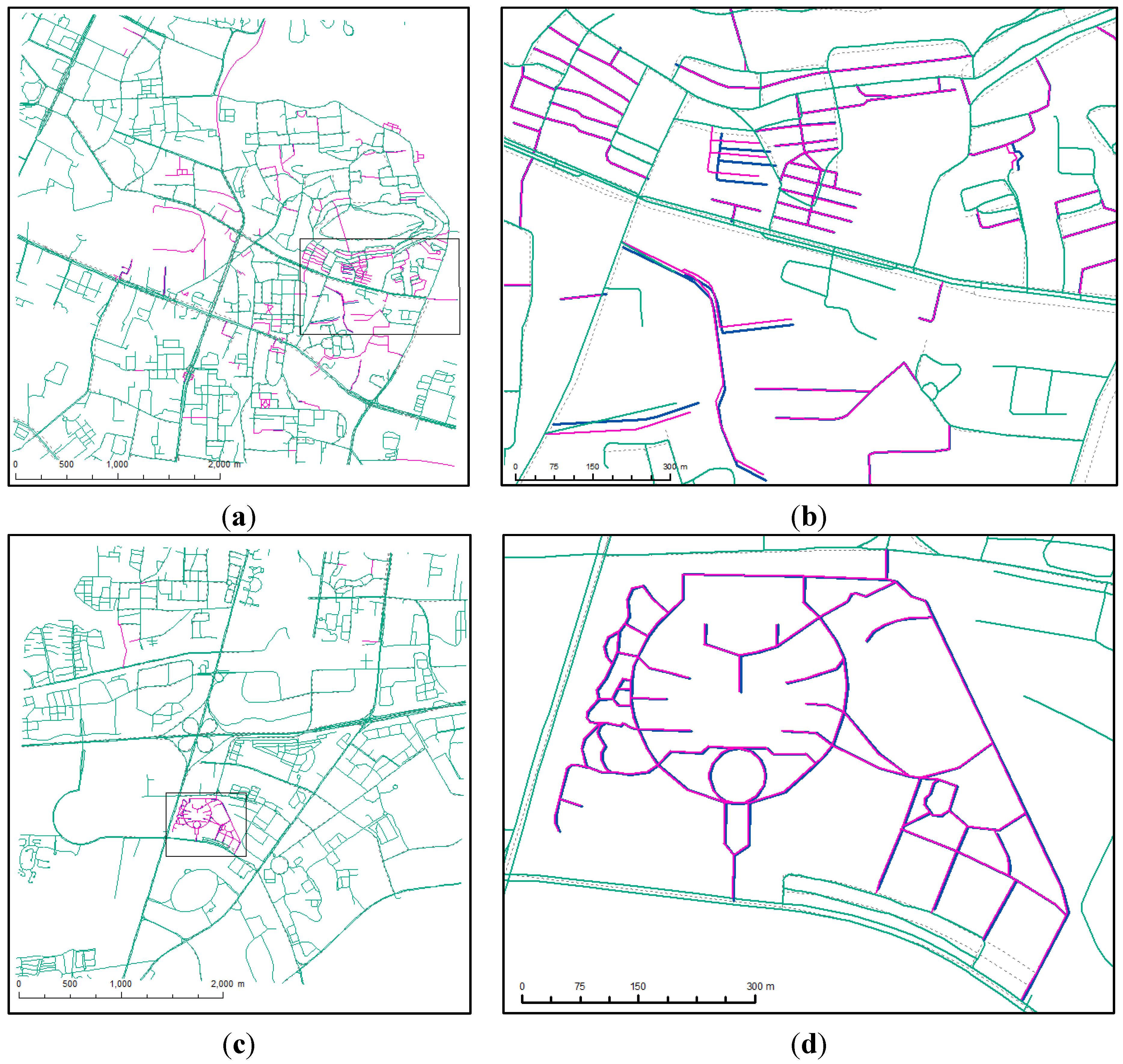
4.1. Optimal Buffers

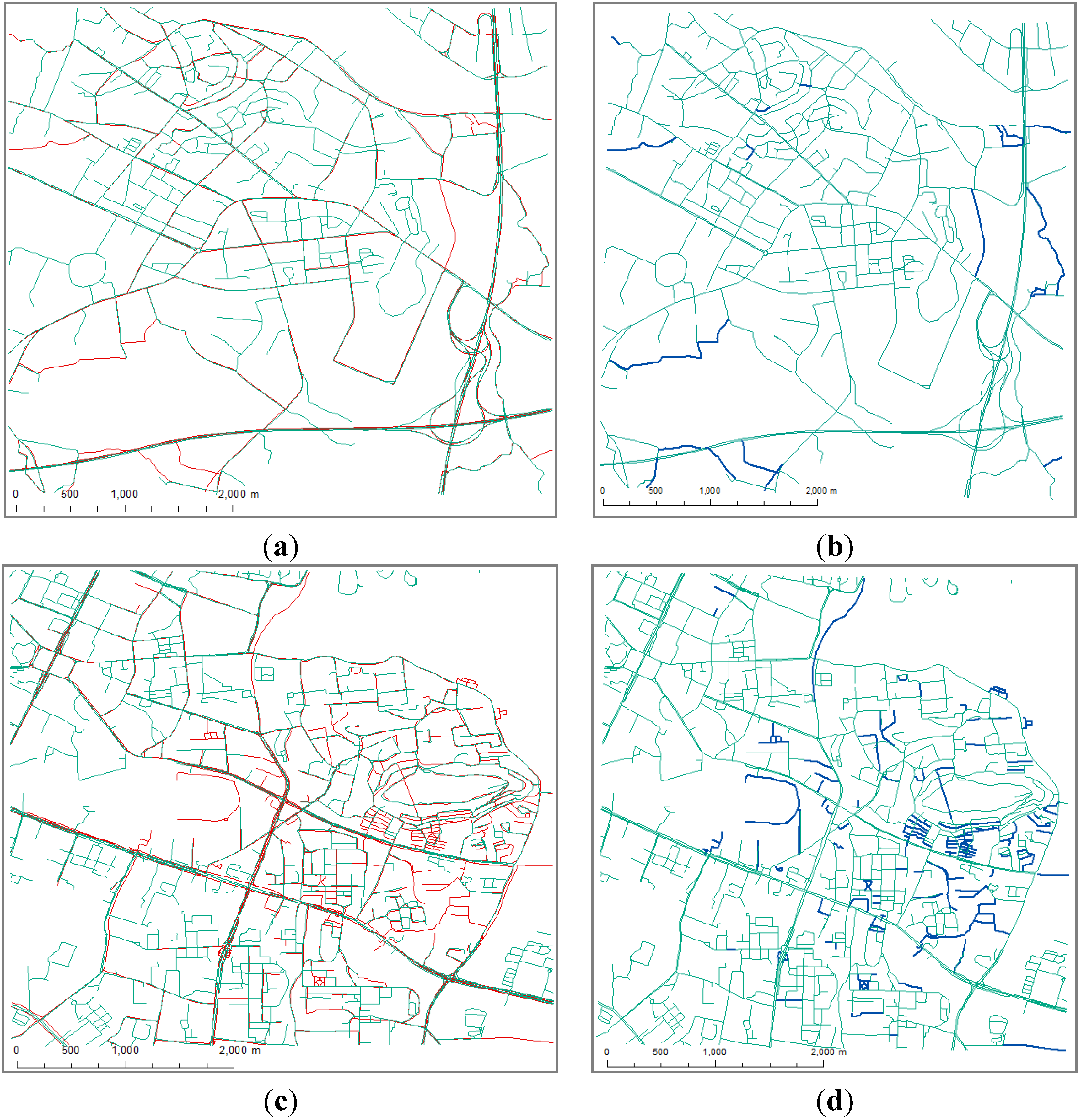
4.2. New Roads Detected


| Datasets | 1 | 2 | 3 | 4 | 5 | Wuhan |
|---|---|---|---|---|---|---|
| Optimal buffer (m) | 20.5 | 22.5 | 22.5 | 22.5 | 16.5 | 22.5 |
| Correctly detected new roads (km) | 7.587 | 5.984 | 35.012 | 21.980 | 10.371 | 52.803 |
| Wrongly detected new roads (km) | 0.022 | 0.297 | 1.581 | 1.406 | 0.134 | 2.456 |
| Missed new roads (km) | 0.135 | 0.090 | 0.589 | 1.117 | 0.322 | 0.808 |
| Precision % | 99.71 | 95.27 | 95.68 | 93.99 | 98.72 | 95.56 |
| Recall % | 98.25 | 98.52 | 98.35 | 95.16 | 96.99 | 98.49 |
4.3. The Updated Reference Roads


| Datasets | 1 | 2 | 3 | 4 | 5 | Wuhan |
|---|---|---|---|---|---|---|
| New roads Length (km) | 7.722 | 6.074 | 35.601 | 23.097 | 10.693 | 2008.644 |
| 5.62 | 2.61 | 19.60 | 9.68 | 5.89 | 11.96 |
5. Conclusion
Acknowledgment
Author Contributions
Conflicts of Interest
References
- Haklay, M.; Singleton, A.; Parker, C. Web mapping 2.0: The neogeography of the Geoweb. Geogr. Compass 2008, 2, 2011–2039. [Google Scholar] [CrossRef]
- Goodchild, M.F. Citizens as sensors: The world of volunteered geography. GeoJournal 2007, 69, 211–221. [Google Scholar] [CrossRef]
- Goodchild, M.F.; Glennona, J.A. Crowdsourcing geographic information for disaster response: A research frontier. Int. J. Digit. Earth 2010, 3, 231–241. [Google Scholar] [CrossRef]
- Haklay, M.; Weber, P. Openstreetmap: User-generated street maps. IEEE Pervasive Comput. 2008, 7, 12–18. [Google Scholar] [CrossRef]
- Flanagin, A.J.; Metzger, M.J. The credibility of volunteered geographic information. GeoJ. 2008, 72, 137–148. [Google Scholar] [CrossRef]
- Ying, F.Y.; Corcoran, P.; Mooney, P.; Winstanley, A. How little is enough? Evaluation of user satisfaction with maps generated by a progressive transmission scheme for geospatial data. In Proceedings of 14th AGILE International Conference on Geographic Information Science, Utrecht, Netherlands, 18–22 April 2011.
- Haklay, M. How good is OpenStreetMap information? A comparative study of OpenStreetMap and ordnance survey datasets for London and the rest of England. Plan. Des. 2010, 37, 682–703. [Google Scholar]
- Ather, A. A Quality Analysis of OpenStreetMap Data. Master’s Thesis, University College London, London, UK, 2009. [Google Scholar]
- Girres, J.-F.; Touya, G. Quality assessment of the French OpenStreetMap dataset. Trans. GIS 2010, 14, 435–459. [Google Scholar] [CrossRef]
- Zielstra, D.; Zipf, A. Quantitative studies on the data quality of OpenStreetMap in Germany. In Proceedings of GIScience 2010: Sixth International Conference on Geographic Information Science, Zurich, Switzerland, 14–17 September 2010.
- Ludwig, I.; Voss, A.; Krause-Traudes, M. A Comparison of the Street Networks of Navteq and OSM in Germany. In Advancing Geoinformation Science for A Changing World; Springer: Heidelberg, Germany, 2011; pp. 65–84. [Google Scholar]
- Kounadi, O. Assessing the Quality of OpenStreetMap Data. Master’s Thesis, University College of London, London, UK, 2009. [Google Scholar]
- Helbich, M.; Amelunxen, C.; Neis, P.; Zipf, A. Comparative spatial analysis of positional accuracy of OpenStreetMap and proprietary geodata. In Proceedings of GI_Forum 2012: Geovisualization Society and Learning, Salzburg, Germany, 4–6 July 2012.
- Fan, H.; Zipf, A.; Fu, Q.; Neis, P. Quality assessment for building footprints data on OpenStreetMap. Int. J. Geogr. Inf. Sci. 2014, 28, 700–719. [Google Scholar] [CrossRef]
- Mooney, P.; Corcoran, P.; Winstanley, A.C. Towards quality metrics for OpenStreetMap. In Proceedings of the 18th SIGSPATIAL International Conference on Advances in Geographic Information Systems, New York, NY, USA, 3–5 November 2010.
- Barron, C.; Neis, P.; Zipf, A. A comprehensive framework for intrinsic OpenStreetMap quality analysis. Trans. GIS 2014, 18, 877–895. [Google Scholar] [CrossRef]
- Chen, S.Y. A Web-Based Accessibility Service OpenStreetMap Data. Master’s Thesis, Shanghai Normal University, Shanghai, China, 2010. [Google Scholar]
- Over, M.; Schilling, A.; Neubauer, S.; Zipf, A. Generating web-based 3D City Models from OpenStreetMap: The current situation in Germany. Comput. Environ. Urban Syst. 2010, 34, 496–507. [Google Scholar] [CrossRef]
- Mondzech, J.; Sester, M. Quality analysis of OpenStreetMap data based on application needs. Int. J. Geogr. Inf. Geovisualization 2011, 46, 115–125. [Google Scholar] [CrossRef]
- Pourabdollah, A.; Morley, J.; Feldman, S.; Jackson, M. Towards an authoritative OpenStreetMap: Conflating OSM and OS Opendata national maps’ road network. ISPRS Int. J. Geo Inf. 2013, 2, 704–728. [Google Scholar] [CrossRef]
- Zhang, Y.F.; Yang, B.; Luan, X. Automated matching crowdsourcing road networks using probabilistic relaxation. In Proceedings of the 2012 XXII ISPRS Congress, Melbourne, ViC, Australia, 25 August–1 September 2012.
- Neis, P.; Zielstra, D. Recent developments and future trends in volunteered geographic information research: The case of OpenStreetMap. Future Internet 2014, 6, 76–106. [Google Scholar] [CrossRef]
- Cobb, M.A.; Chung, M.J.; Foley, H.; Petry, F.E.; Shaw, K.B.; Miller, H.V. A rule-based approach for the conflation of attributed vector data. Geoinformatica 1998, 2, 7–35. [Google Scholar] [CrossRef]
- Jiang, J.; CHEN, J. Some Consideration for Update of Fundamental Geoinformation Database. Bull. Surv. Mapp. 2000, 5, 1–3. [Google Scholar]
- Rosen, B.; Saalfeld, A. Match criteria for automatic alignment. In Proceedings of Auto-Carto VII, Washington, DC, USA, 11–14 March 1985.
- Volz, S. An iterative approach for matching multiple representations of street data. In Proceedings of 2006 ISPRS Workshop on Multiple Representation And Interoperability Of Spatial Data, Hannover, Germany, 22–24 February 2006.
- Xiong, D.; Sperling, J. Semiautomated matching for network database integration. ISPRS J. Photogramm. Remote. Sens. 2004, 59, 35–46. [Google Scholar] [CrossRef]
- Zhang, M.; Meng, L. An iterative road-matching approach for the integration of postal data. Comput. Environ. Urban Syst. 2007, 31, 597–615. [Google Scholar] [CrossRef]
- Ruiz, J.J.; Ariza, F.J.; Ureña, M.A.; Blázquez, E.B. Digital map conflation: A review of the process and a proposal for classification. Int. J. Geogr. Inf. Sci. 2011, 25, 1439–1466. [Google Scholar] [CrossRef]
- Gabay, Y.; Doytsher, Y. Automatic adjustment of line maps. In Proceedings of GIS/LIS’ 94 Annual Convention, Phoenix, AZ, USA; 1994. [Google Scholar]
- Walter, V.; Fritsch, D. Matching spatial data sets: A statistical approach. International Journal of Geographical Information Science 1999, 13, 445–473. [Google Scholar] [CrossRef]
- Gösseln, G.V. A matching approach for the integration, change detection and adaptation of heterogeneous vector data sets. In Proceedings of XXII International Cartography Conference, Coruña, Spain, 9–16 July 2005.
- Wiki. Roundabout. Available online, https://en.wikipedia.org/wiki/Roundabout (accessed on 20 May 2015).
- Levenshtein, V.I. Binary codes capable of correcting deletions, insertions, and reversals. Sov. Phys. Dokl. 1966, 10, 707–710. [Google Scholar]
© 2015 by the authors; licensee MDPI, Basel, Switzerland. This article is an open access article distributed under the terms and conditions of the Creative Commons Attribution license (http://creativecommons.org/licenses/by/4.0/).
Share and Cite
Liu, C.; Xiong, L.; Hu, X.; Shan, J. A Progressive Buffering Method for Road Map Update Using OpenStreetMap Data. ISPRS Int. J. Geo-Inf. 2015, 4, 1246-1264. https://0-doi-org.brum.beds.ac.uk/10.3390/ijgi4031246
Liu C, Xiong L, Hu X, Shan J. A Progressive Buffering Method for Road Map Update Using OpenStreetMap Data. ISPRS International Journal of Geo-Information. 2015; 4(3):1246-1264. https://0-doi-org.brum.beds.ac.uk/10.3390/ijgi4031246
Chicago/Turabian StyleLiu, Changyong, Lian Xiong, Xiangyun Hu, and Jie Shan. 2015. "A Progressive Buffering Method for Road Map Update Using OpenStreetMap Data" ISPRS International Journal of Geo-Information 4, no. 3: 1246-1264. https://0-doi-org.brum.beds.ac.uk/10.3390/ijgi4031246