Extraction of Pluvial Flood Relevant Volunteered Geographic Information (VGI) by Deep Learning from User Generated Texts and Photos


Abstract
:1. Introduction
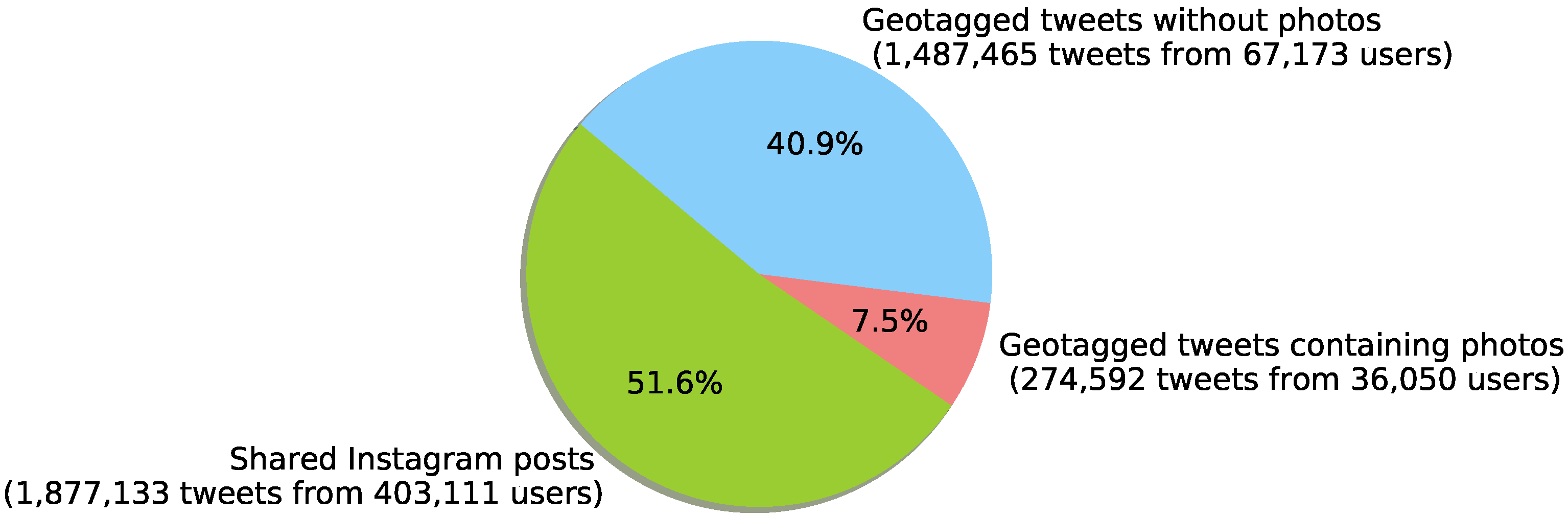
2. Social Media Data Acquisition
3. Related Methods for Interpreting Flood Relevant Social Media Information
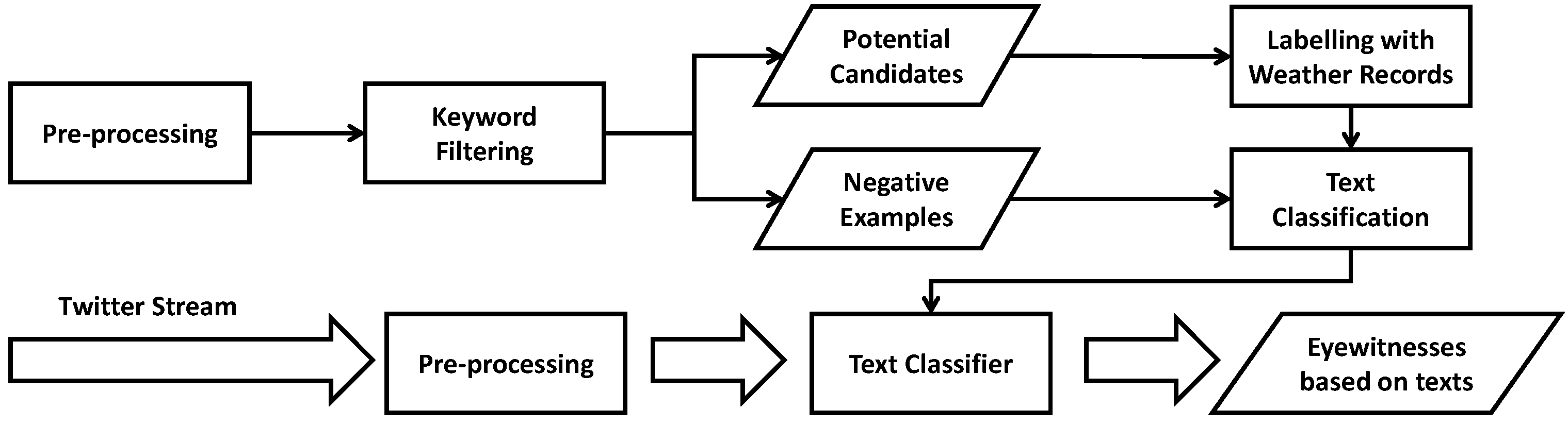
4. Interpretation of Social Media Texts
4.1. Pre-Processing and Training Preparation
4.2. Training of Text Classifiers
4.2.1. Classical NLP Methods
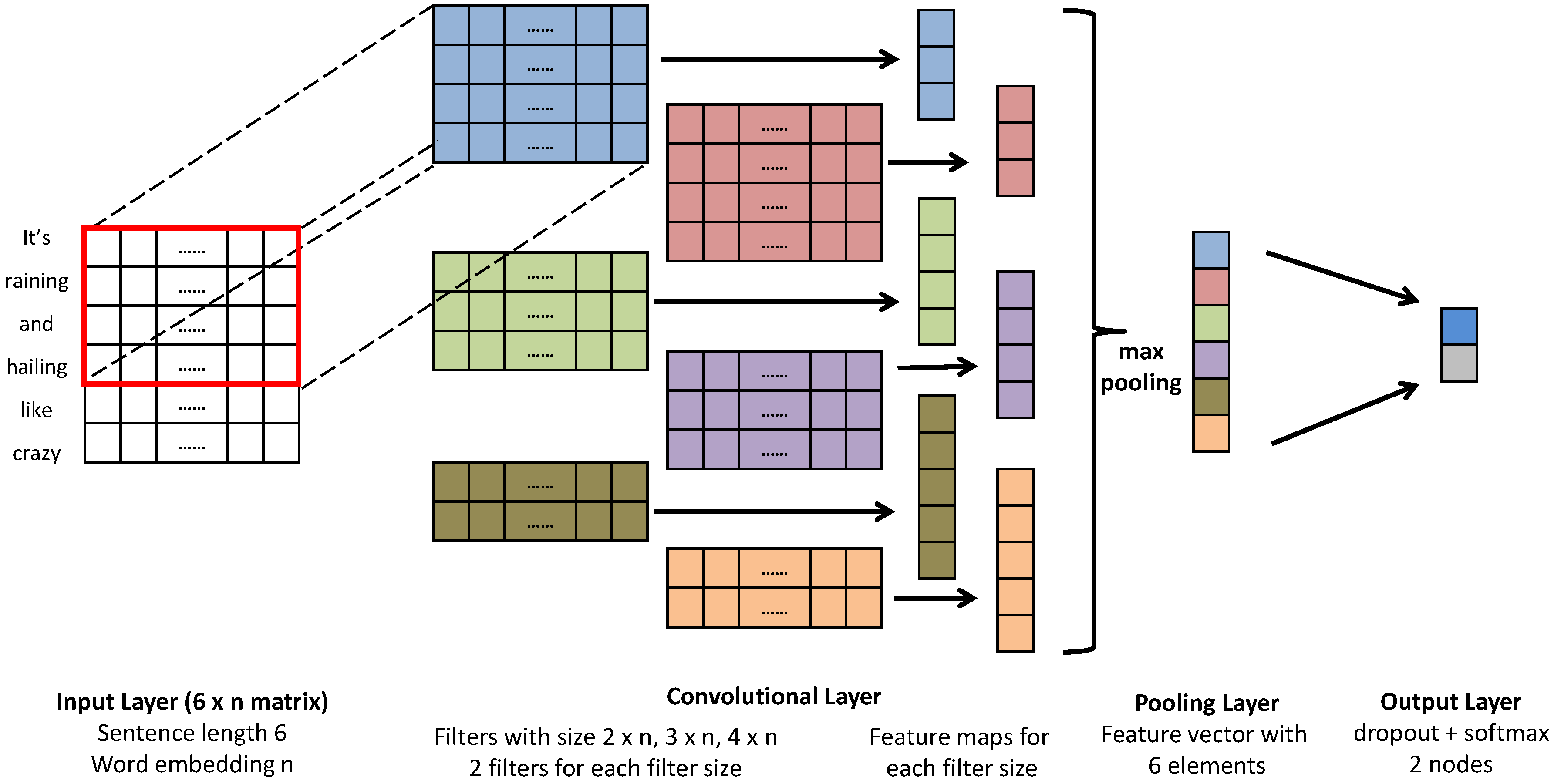
4.2.2. ConvNets for Sentence Classification
4.3. Results and Evaluation
5. Interpretation of Social Media Photos
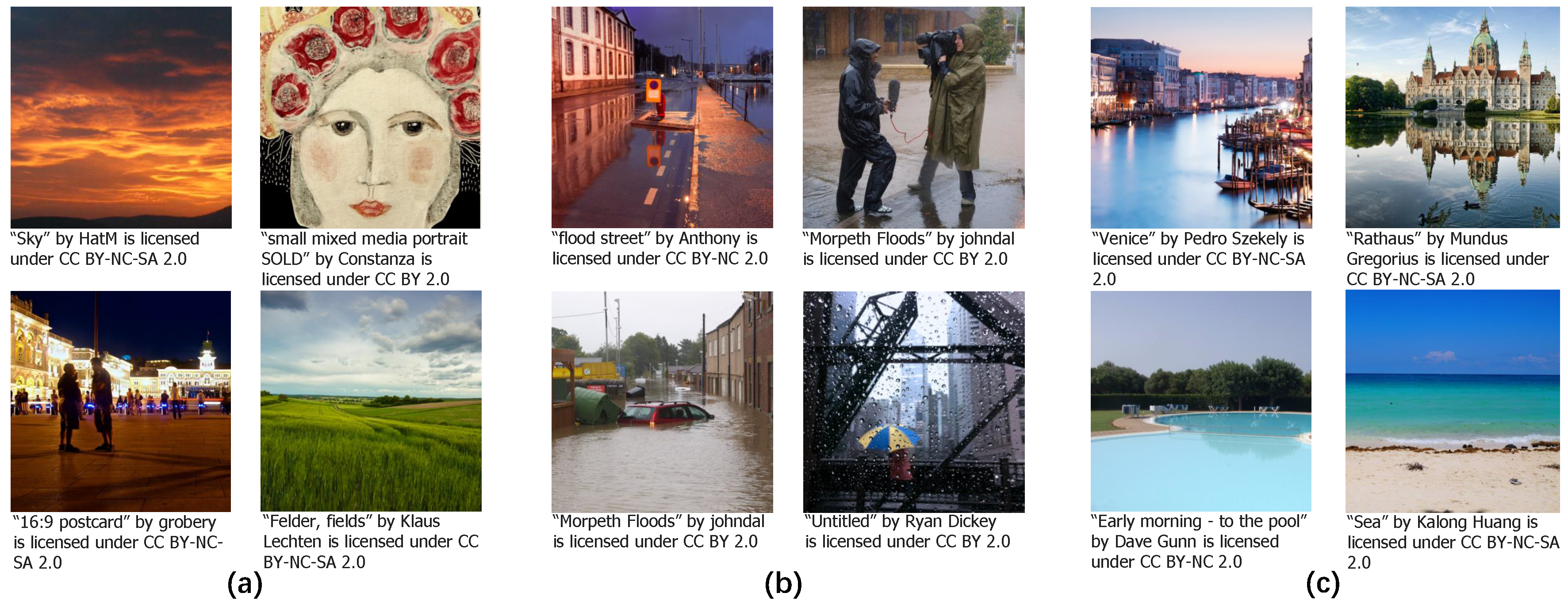
5.1. Input Training Dataset
5.2. Training of Image Classifiers
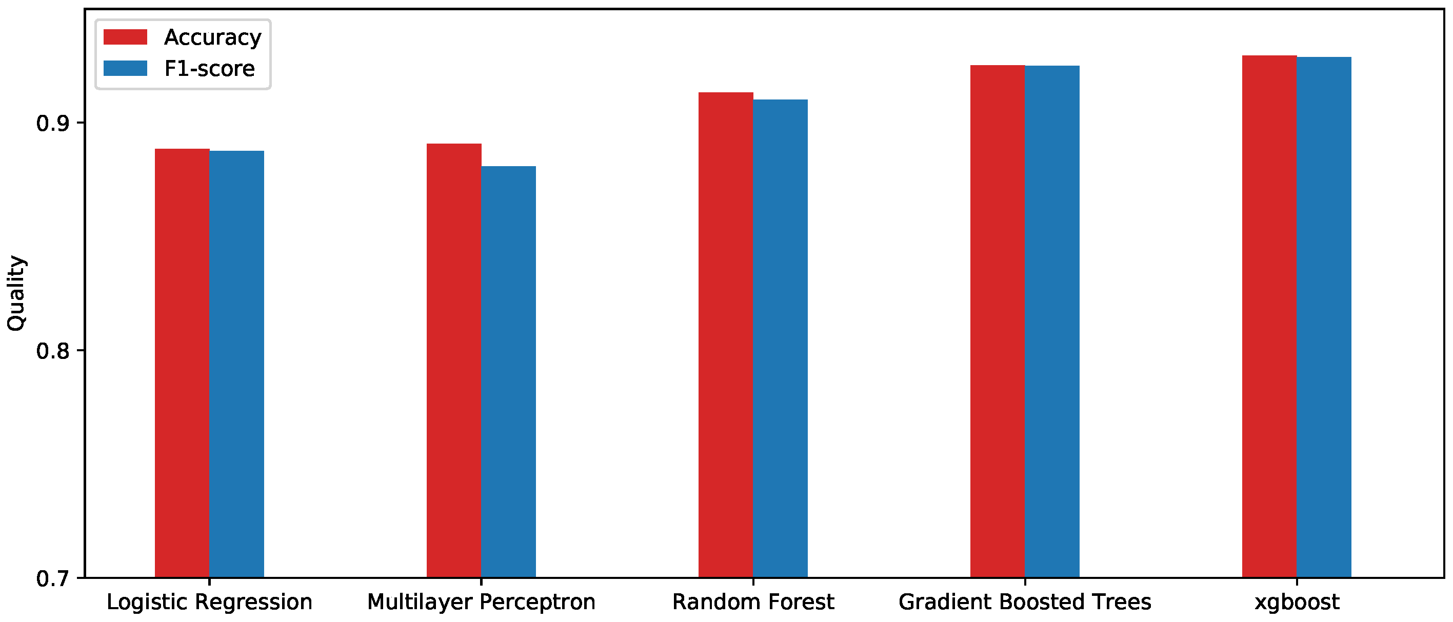
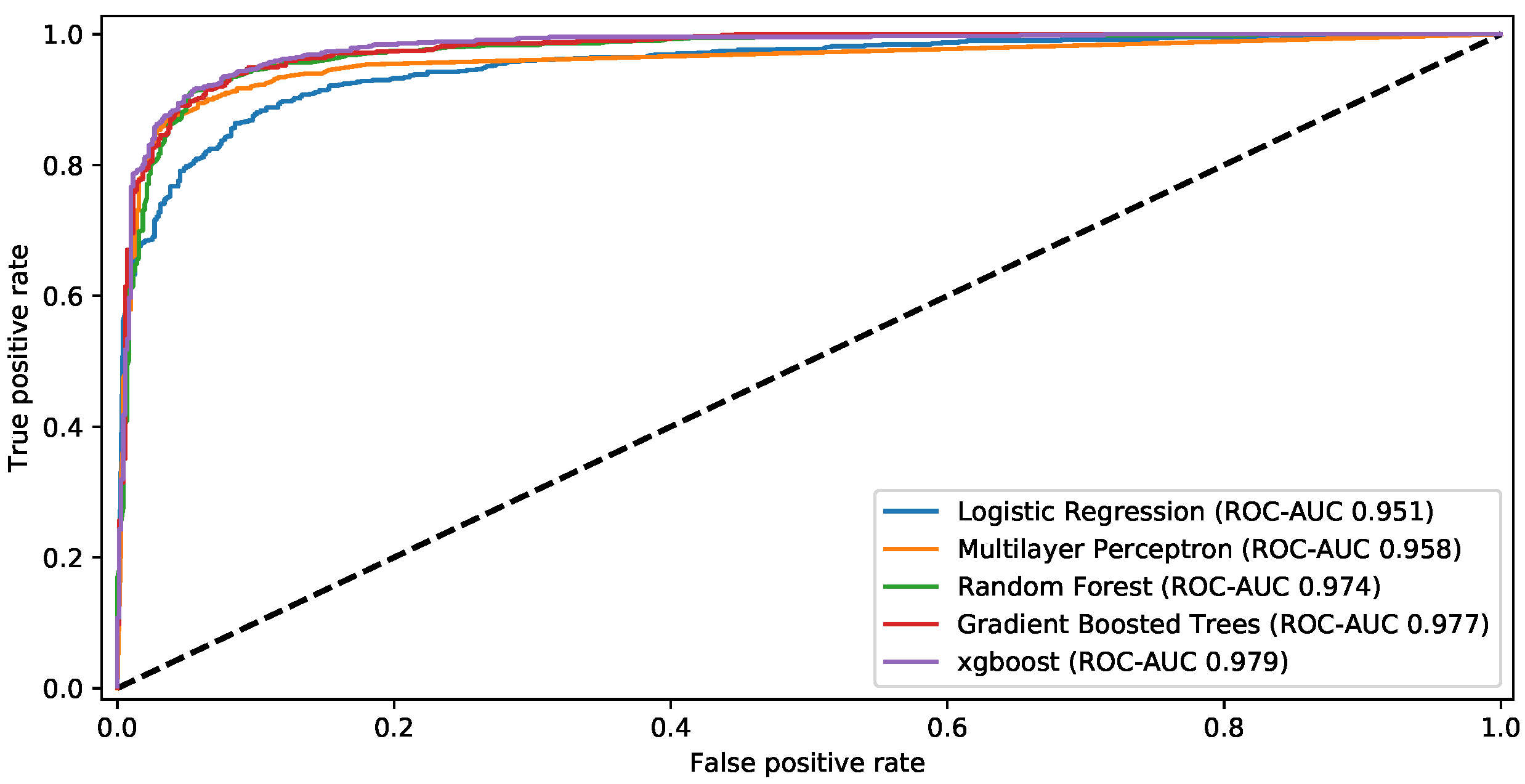
5.3. Results and Evaluations
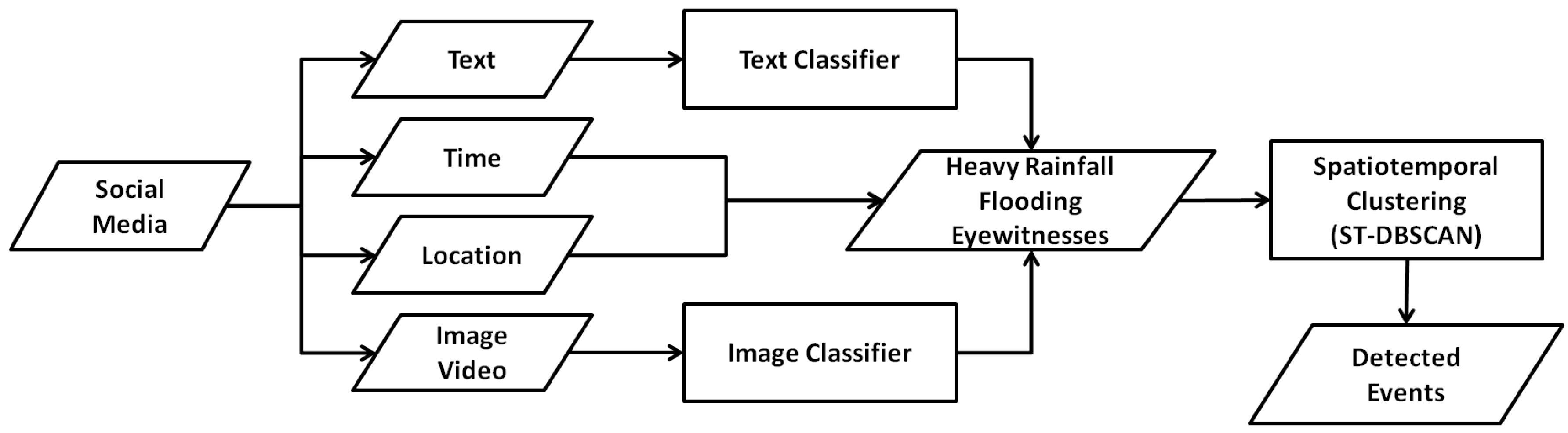
6. Detection of Heavy Rainfall and Flooding Events
6.1. Event Detection with Spatiotemporal Clustering
6.2. Polygon Based Hot Spot Detection with Getis-Ord Gi*
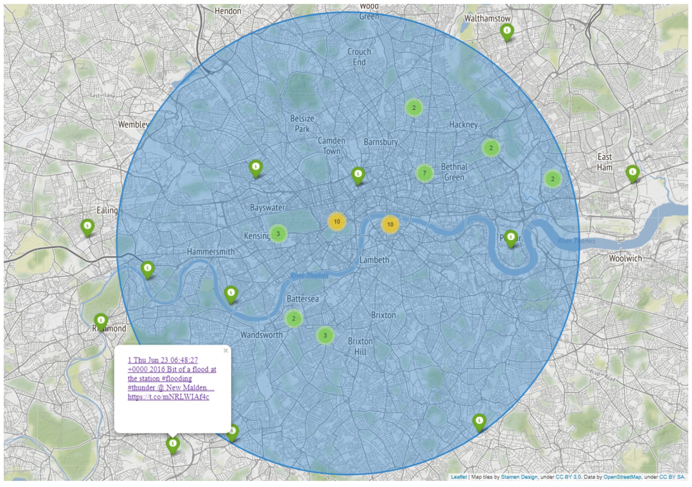
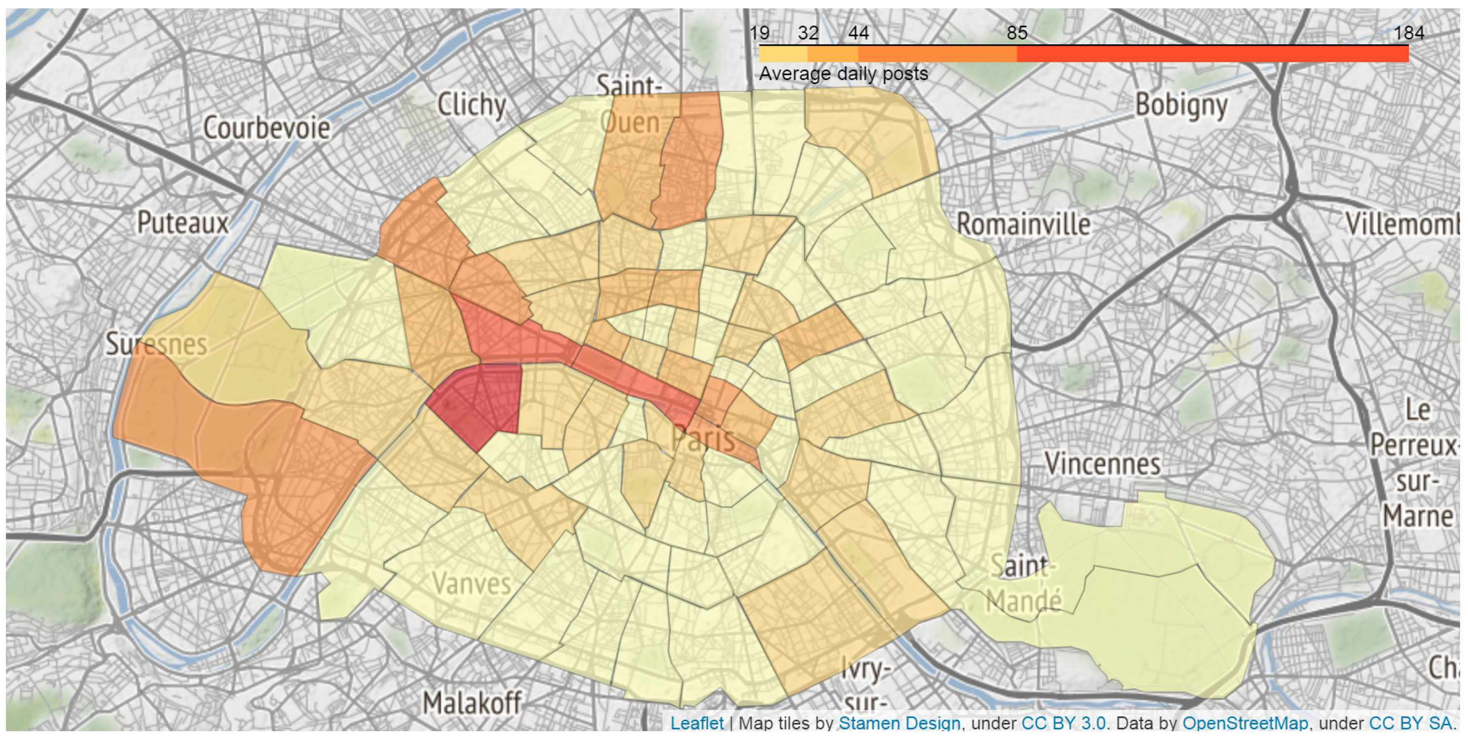
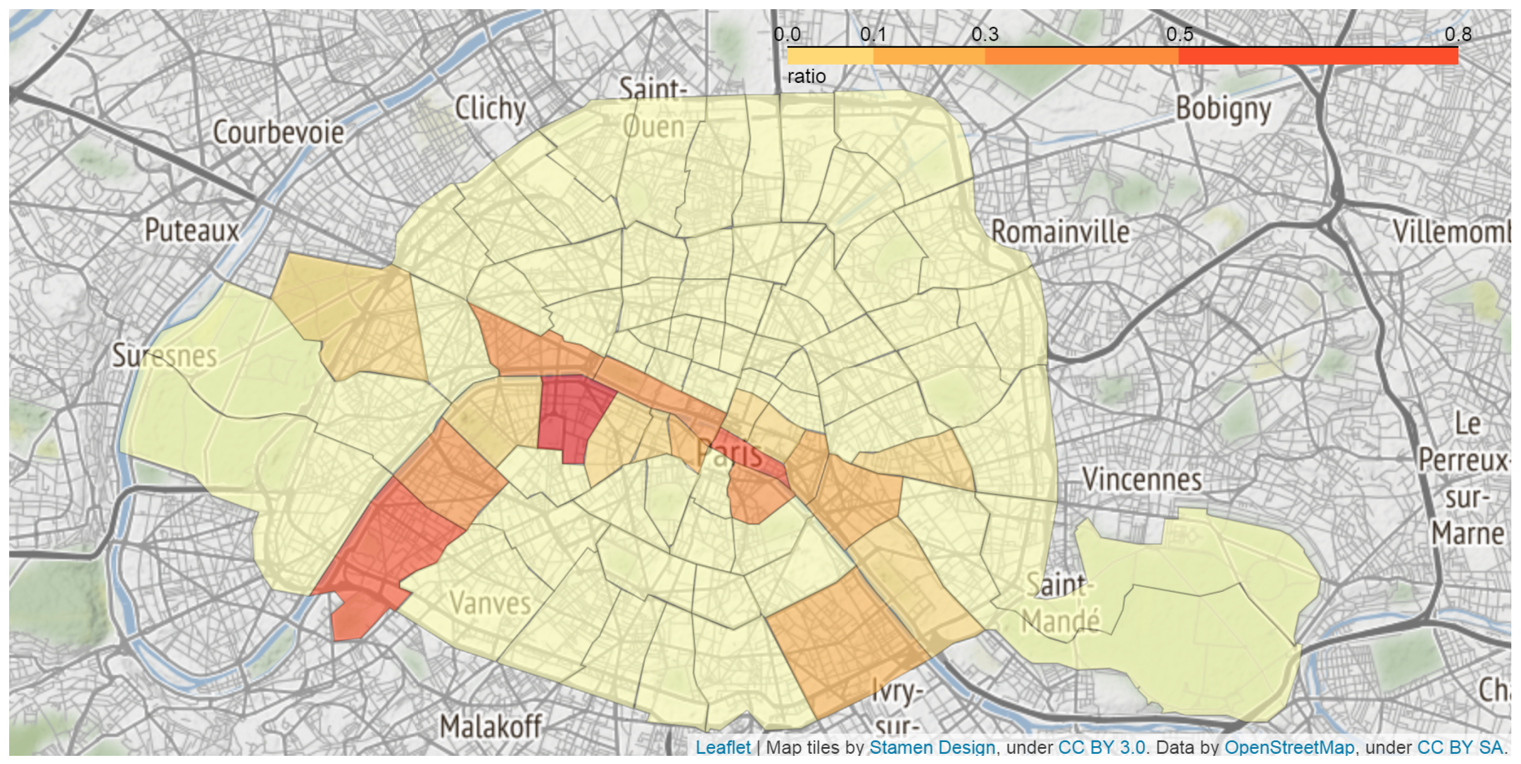
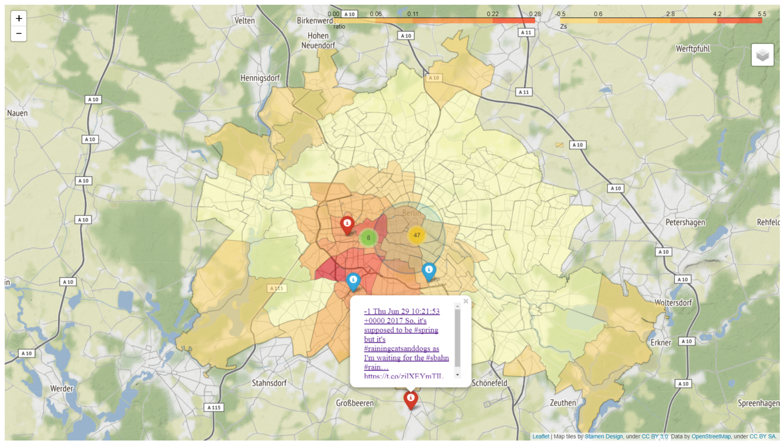
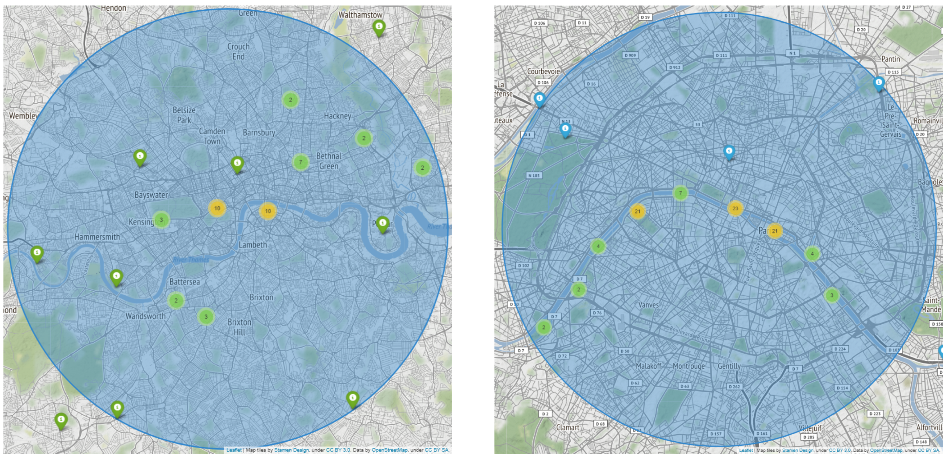
7. Visualization of the Pluvial Flood Relevant Information
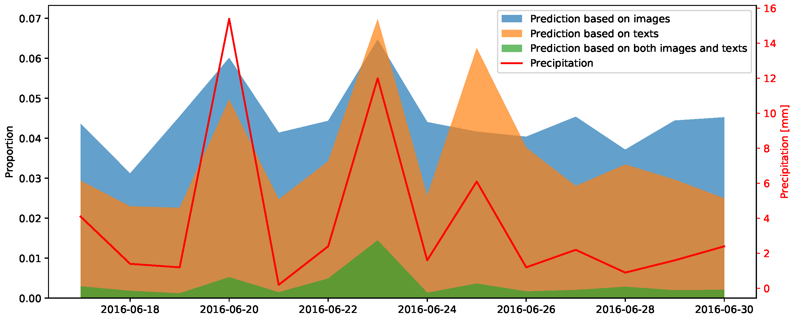
8. Analyses and Comparison with External Data Source
9. Conclusions
Acknowledgments
Author Contributions
Conflicts of Interest
Abbreviations
| AUC | Area Under the Curve |
| ConvNets | Convolutional Neural Networks |
| LDA | Latent Dirichlet allocation |
| NLP | Natural Language Processing |
| NLTK | Natural Language Toolkit |
| RBF | Radial Basis Function |
| ROC | Receiver Operating Characteristic |
| SVM | Support Vector Machine |
| tf-idf | Term Frequency - Inverse Document Frequency |
| VGI | Volunteered Geographic Information |
References
- Three Common Types of Flood Explained. Available online: http://www.intermap.com/risks-of-hazard-blog/three-common-types-of-flood-explained (accessed on 7 November 2017).
- Shoothill GaugeMap. Available online: http://www.gaugemap.co.uk/ (accessed on 7 November 2017).
- NOAA Tides & Currents. Available online: https://tidesandcurrents.noaa.gov/ (accessed on 7 November 2017).
- Real-Time Prediction of Pluvial Floods and Induced Water Contamination in Urban Areas. Available online: https://www.pluvialfloods.uni-hannover.de/pluvialfloods0.html?&L=1 (accessed on 7 November 2017).
- Wang, Y.; Wang, T.; Ye, X.; Zhu, J.; Lee, J. Using social media for emergency response and urban sustainability: A case study of the 2012 Beijing rainstorm. Sustainability 2016, 8, 25. [Google Scholar] [CrossRef]
- Zu viel Wasser für Berlin: Stadt Versinkt im Verkehrs-Chaos—B.Z. Berlin. Available online: http://www.bz-berlin.de/berlin/unwetterwarnung-berlin-wetter (accessed on 7 November 2017).
- Netatmo. Available online: https://www.netatmo.com/ (accessed on 7 November 2017).
- Google Flue Trend. Available online: https://www.google.org/flutrends/about/ (accessed on 7 November 2017).
- Ginsberg, J.; Mohebbi, M.; Patel, R.; Brammer, L.; Smolinski, M.; Brilliant, L. Detecting influenza epidemics using search engine query data. Nature 2009, 457, 1012–1014. [Google Scholar] [CrossRef] [PubMed]
- Lazer, D.; Kennedy, R.; King, G.; Vespignani, A. The parable of Google Flu: Traps in big data analysis. Science 2014, 343, 1203–1205. [Google Scholar] [CrossRef] [PubMed] [Green Version]
- Goodchild, M.F. Citizens as sensors: The world of volunteered geography. GeoJournal 2007, 69, 211–221. [Google Scholar] [CrossRef]
- Zook, M.; Graham, M.; Shelton, T.; Gorman, S. Volunteered geographic information and crowdsourcing disaster relief: A case study of the Haitian earthquake. World Med. Health Policy 2010, 2, 7–33. [Google Scholar] [CrossRef]
- Sakaki, T.; Okazaki, M.; Matsuo, Y. Earthquake shakes Twitter users: Real-time event detection by social sensors. In Proceedings of the 19th International Conference on World Wide Web, Raleigh, NC, USA, 26–30 April 2010; ACM: New York, NY, USA, 2010; pp. 851–860. [Google Scholar]
- Earle, P.S.; Bowden, D.C.; Guy, M. Twitter earthquake detection: Earthquake monitoring in a social world. Ann. Geophys. 2011, 54, 708–715. [Google Scholar] [CrossRef]
- Crooks, A.; Croitoru, A.; Stefanidis, A.; Radzikowski, J. #Earthquake: Twitter as a Distributed Sensor System. Trans. GIS 2013, 17, 124–147. [Google Scholar] [CrossRef]
- Herfort, B.; de Albuquerque, J.P.; Schelhorn, S.J.; Zipf, A. Exploring the geographical relations between social media and flood phenomena to improve situational awareness. In Connecting a Digital Europe through Location and Place; Huerta, J., Schade, S., Granell, C., Eds.; Springer: Cham, Switzerland, 2014; pp. 55–71. [Google Scholar]
- Schnebele, E.; Cervone, G. Improving remote sensing flood assessment using volunteered geographical data. Nat. Hazards Earth Syst. Sci. 2013, 13, 669–677. [Google Scholar] [CrossRef]
- Terpstra, T.; Stronkman, R.; de Vries, A.; Paradies, G.L. Towards a realtime Twitter analysis during crises for operational crisis management. In Proceedings of the 9th International ISCRAM Conference, Vancouver, BC, Canada, 22–25 April 2012; Simon Fraser University: Vancouver, BC, Canada, 2012. [Google Scholar]
- De Longueville, B.; Smith, R.S.; Luraschi, G. “OMG, from here, I can see the flames!”: A use case of mining Location Based Social Networks to acquire spatiotemporal data on forest fires. In Proceedings of the 2009 International Workshop on Location Based Social Networks—LBSN’09, Seattle, WA, USA, 3 November 2009; ACM: New York, NY, USA, 2009. [Google Scholar]
- Wang, Z.; Ye, X.; Tsou, M.H. Spatial, temporal, and content analysis of Twitter for wildfire hazards. Nat. Hazards 2016, 83, 523–540. [Google Scholar] [CrossRef]
- De Longueville, B.; Luraschi, G.; Smits, P.; Peedell, S.; Groeve, T.D. Citizens as sensors for natural hazards: A VGI integration workflow. Geomatica 2010, 64, 41–59. [Google Scholar]
- Fuchs, G.; Andrienko, N.; Andrienko, G.; Bothe, S.; Stange, H. Tracing the German centennial flood in the stream of tweets: first lessons learned. In Proceedings of the Second ACM SIGSPATIAL International Workshop on Crowdsourced and Volunteered Geographic Information, Orlando, FL, USA, 5–8 November 2013; ACM: New York, NY, USA, 2013; pp. 31–38. [Google Scholar]
- Li, Z.; Wang, C.; Emrich, C.T.; Guo, D. A novel approach to leveraging social media for rapid flood mapping: A case study of the 2015 South Carolina floods. Cartogr. Geogr. Inf. Sci. 2017, 45, 97–110. [Google Scholar] [CrossRef]
- Karimi, S.; Yin, J.; Paris, C. Classifying Microblogs for Disasters. In Proceedings of the 18th Australasian Document Computing Symposium, Brisbane, Australia, 5–6 December 2013; ACM: New York, NY, USA, 2013; pp. 26–33. [Google Scholar]
- Feng, Y.; Sester, M. Social media as a rainfall indicator. In Proceedings of the Societal Geo-Innovation: Short Papers, Posters and Poster Abstracts of the 20th AGILE Conference on Geographic Information Science, Wageningen, The Netherlands, 9–12 May 2017; Bregt, A., Sarjakoski, T., van Lammeren, R., Rip, F., Eds.; Wageningen University & Research: Wageningen, The Netherlands, 2017. [Google Scholar]
- Fohringer, J.; Dransch, D.; Kreibich, H.; Schröter, K. Social media as an information source for rapid flood inundation mapping. Nat. Hazards Earth Syst. Sci. 2015, 15, 2725–2738. [Google Scholar] [CrossRef]
- Bischke, B.; Bhardwaj, P.; Gautam, A.; Helber, P.; Borth, D.; Dengel, A. Detection of Flooding Events in Social Multimedia and Satellite Imagery using Deep Neural Networks. In Proceedings of the Working Notes Proceeding MediaEval Workshop, Dublin, Ireland, 13–15 September 2017. [Google Scholar]
- Avgerinakis, K.; Moumtzidou, A.; Andreadis, S.; Michail, E.; Gialampoukidis, I.; Vrochidis, S.; Kompatsiaris, I. Visual and textual analysis of social media and satellite images for flood detection@ multimedia satellite task MediaEval 2017. In Proceedings of the Working Notes Proceeding MediaEval Workshop, Dublin, Ireland, 13–15 September 2017. [Google Scholar]
- Silvestro, F.; Gabellani, S.; Giannoni, F.; Parodi, A.; Rebora, N.; Rudari, R.; Siccardi, F. A hydrological analysis of the 4 November 2011 event in Genoa. Nat. Hazards Earth Syst. Sci. 2012, 12, 2743–2752. [Google Scholar] [CrossRef] [Green Version]
- Twitter: Number of Monthly Active Users 2010–2017. Available online: https://0-www-statista-com.brum.beds.ac.uk/statistics/282087/number-of-monthly-active-twitter-users/ (accessed on 7 November 2017).
- Twitter-Docs. Available online: https://dev.twitter.com/streaming/overview (accessed on 7 November 2017).
- Twitter. Rate Limiting. Available online: https://developer.twitter.com/en/docs/basics/rate-limiting (accessed on 7 November 2017).
- MongoDB for GIANT Ideas. Available online: https://www.mongodb.com/ (accessed on 7 November 2017).
- Moniruzzaman, A.B.M.; Hossain, S.A. Nosql database: New era of databases for big data analytics-classification, characteristics and comparison. arXiv, 2013; arXiv:1307.0191. [Google Scholar]
- Dittrich, A.; Lucas, C. Is This Twitter Event a Disaster? In Proceedings of the AGILE’2014 International Conference on Geographic Information Science, Connecting a Digital Europe through Location and Place, Castellón, Spain, 3–6 June 2014. [Google Scholar]
- LeCun, Y.; Bengio, Y. Convolutional networks for images, speech, and time series. In The Handbook of Brain Theory and Neural Networks; MIT Press: Cambridge, MA, USA, 1995; pp. 255–258. [Google Scholar]
- Krizhevsky, A.; Sutskever, I.; Hinton, G.E. Imagenet classification with deep convolutional neural networks. In Advances in Neural Information Processing Systems; Curran Associates, Inc.: Red Hook, NY, USA, 2012; pp. 1097–1105. [Google Scholar]
- ImageNet. Available online: http://www.image-net.org/ (accessed on 7 November 2017).
- Donahue, J.; Jia, Y.; Vinyals, O.; Hoffman, J.; Zhang, N.; Tzeng, E.; Darrell, T. DeCAF: A Deep Convolutional Activation Feature for Generic Visual Recognition. In Proceedings of the 31st International Conference on Machine Learning (ICML-14), Beijing, China, 21–26 June 2014; pp. 647–655. [Google Scholar]
- Yosinski, J.; Clune, J.; Bengio, Y.; Lipson, H. How transferable are features in deep neural networks? In Proceedings of the Advances in Neural Information Processing Systems 27, Montreal, QC, Canada, 8–13 December 2014; Ghahramani, Z., Welling, M., Cortes, C., Lawrence, N.D., Weinberger, K.Q., Eds.; MIT Press: Cambridge, MA, USA, 2014; pp. 3320–3328. [Google Scholar]
- Goodfellow, I.; Bengio, Y.; Courville, A. Section 15.2—Transfer Learning and Domain Adaptation. In Deep Learning; MIT Press: Cambridge, MA, USA, 2016; pp. 328–343. [Google Scholar]
- Nogueira, K.; Penatti, O.A.; dos Santos, J.A. Towards better exploiting convolutional neural networks for remote sensing scene classification. Pattern Recognit. 2017, 61, 539–556. [Google Scholar] [CrossRef]
- Niessner, R.; Schilling, H.; Jutzi, B. Investigations on the potential of Convolutional Neural Networks for vehicle classification based on RGB and Lidar data. ISPRS Ann. Photogramm. Remote Sens. Spat. Inf. Sci. 2017, 4, 115–123. [Google Scholar] [CrossRef]
- Ammour, N.; Alhichri, H.; Bazi, Y.; Benjdira, B.; Alajlan, N.; Zuair, M. Deep Learning Approach for Car Detection in UAV Imagery. Remote Sens. 2017, 9, 312. [Google Scholar] [CrossRef]
- Iannelli, G.C.; Dell’Acqua, F. Extensive Exposure Mapping in Urban Areas through Deep Analysis of Street-Level Pictures for Floor Count Determination. Urban Sci. 2017, 1, 16. [Google Scholar] [CrossRef]
- Zamir, A.R.; Hakeem, A.; Van Gool, L.; Shah, M.; Szeliski, R. Introduction to Large-Scale Visual Geo-localization. In Large-Scale Visual Geo-Localization; Springer: Berlin, Germnay, 2016; pp. 1–18. [Google Scholar]
- Huang, Q.; Xiao, Y. Geographic Situational Awareness: Mining Tweets for Disaster Preparedness, Emergency Response, Impact, and Recovery. ISPRS Int. J. Geoinf. 2015, 4, 1549–1568. [Google Scholar] [CrossRef]
- Manning, C.D.; Raghavan, P.; Schütze, H. Section 6.2—Term frequency and weighting. In Introduction to Information Retrieval; Cambridge University Press: New York, NY, USA, 2008; pp. 107–109. [Google Scholar]
- Kim, Y. Convolutional neural networks for sentence classification. In Proceedings of the 2014 Conference on Empirical Methods in Natural Language Processing (EMNLP), Doha, Qatar, 25–29 October 2014; pp. 1746–1751. [Google Scholar]
- Mikolov, T.; Sutskever, I.; Chen, K.; Corrado, G.S.; Dean, J. Distributed representations of words and phrases and their compositionality. In Advances in Neural Information Processing Systems 26; Curran Associates, Inc.: Red Hook, NY, USA, 2013; pp. 3111–3119. [Google Scholar]
- Lin, Z.; Jin, H.; Robinson, B.; Lin, X. Towards an accurate social media disaster event detection system based on deep learning and semantic representation. In Proceedings of the 14th Australasian Data Mining Conference, Canberra, Australia, 6–8 December 2016. [Google Scholar]
- Google Code Archive—Stop-Words. Available online: https://code.google.com/archive/p/stop-words/ (accessed on 7 November 2017).
- Natural Language Toolkit. Available online: http://www.nltk.org/ (accessed on 7 November 2017).
- Patrini, G.; Rozza, A.; Menon, A.; Nock, R.; Qu, L. Making Neural Networks Robust to Label Noise: A Loss Correction Approach. In Proceedings of the IEEE Conference on Computer Vision and Pattern Recognition (CVPR), Honolulu, HI, USA, 21–26 July 2017. [Google Scholar]
- Wunderground—Weather Underground. Available online: https://www.wunderground.com/ (accessed on 7 November 2017).
- Weather API: Introduction. Available online: https://www.wunderground.com/weather/api/d/docs (accessed on 7 November 2017).
- Wei, Q.; Dunbrack, R.L., Jr. The role of balanced training and testing data sets for binary classifiers in bioinformatics. PLoS ONE 2013, 8, e67863. [Google Scholar] [CrossRef] [PubMed]
- McCallum, A.; Nigam, K. A comparison of event models for naive Bayes text classification. In Proceedings of the AAAI-98 Workshop on Learning for Text Categorization, Madison, WI, USA, 26–30 July 1998; pp. 41–48. [Google Scholar]
- Breiman, L. Random forests. Mach. Learn. 2001, 45, 5–32. [Google Scholar] [CrossRef]
- Dumais, S.; Platt, J.; Hecherman, D.; Sahami, M. Inductive Learning Algorithms and Representations for Text Categorization. In Proceedings of the 7th International Conference on Information and Knowledge Management, Washington, DC, USA, 2–7 November 1998; pp. 148–155. [Google Scholar]
- Joachims, T. Text categorization with support vector machines: learning with many relevant features. In Machine Learning: ECML 1998; Nédellec, C., Rouveirol, C., Eds.; Springer: Berlin/Heidelberg, Germany, 1998; Volume 1398, pp. 137–142. [Google Scholar]
- Genkin, A.; Lewis, D.D.; Madigan, D. Large-scale Bayesian logistic regression for text categorization. Technometrics 2007, 49, 291–304. [Google Scholar] [CrossRef]
- Pedregosa, F.; Varoquaux, G.; Gramfort, A.; Michel, V.; Thirion, B.; Grisel, O.; Blondel, M.; Prettenhofer, P.; Weiss, R.; Dubourg, V.; et al. Scikit-learn: Machine Learning in Python. J. Mach. Learn. Res. 2011, 12, 2825–2830. [Google Scholar]
- Deep Learning with Word2vec. Available online: https://radimrehurek.com/gensim/models/word2vec.html (accessed on 7 November 2017).
- TensorFlow. Available online: https://www.tensorflow.org/ (accessed on 7 November 2017).
- Zhang, Y.; Wallace, B. A Sensitivity Analysis of (and Practitioners’ Guide to) Convolutional Neural Networks for Sentence Classification. Available online: https://arxiv.org/abs/1510.03820 (accessed on 7 November 2017).
- Szegedy, C.; Vanhoucke, V.; Ioffe, S.; Shlens, J.; Wojna, Z. Rethinking the Inception Architecture for Computer Vision. In Proceedings of the 2016 IEEE Conference on Computer Vision and Pattern Recognition (CVPR), Las Vegas, NV, USA, 27–30 June 2016; pp. 2818–2826. [Google Scholar]
- Pre-Trained GoogLeNet (Inception-V3). Available online: http://download.tensorflow.org/models/image/imagenet/inception-2015-12-05.tgz (accessed on 7 November 2017).
- Friedman, J. Greedy Function Approximation: A Gradient Boosting Machine. Ann. Stat. 2001, 29, 1189–1232. [Google Scholar] [CrossRef]
- Chen, T.; Guestrin, C. Xgboost: A Scalable Tree Boosting System. In Proceedings of the 22nd ACM SIGKDD International Conference on Knowledge Discovery and Data Mining, San Francisco, CA, USA, 13–17 August 2016; ACM: New York, NY, USA, 2016; pp. 785–794. [Google Scholar]
- Ord, J.K.; Getis, A. Local spatial autocorrelation statistics: distributional issues and an application. Geogr. Anal. 1995, 27, 286–306. [Google Scholar] [CrossRef]
- Birant, D.; Kut, A. ST-DBSCAN: An algorithm for clustering spatial-temporal data. Data Knowl. Eng. 2007, 60, 208–221. [Google Scholar] [CrossRef]
- Ester, M.; Kriegel, H.P.; Sander, J.; Xu, X. A density-based algorithm for discovering clusters in large spatial databases with noise. In Proceedings of the International Conference Knowledge Discovery and Data Mining (KKD’96), Portland, OR, 2–4 August 1996; pp. 226–231. [Google Scholar]
- Begum, S.; Otung, I.E. Rain cell size distribution inferred from rain gauge and radar data in the UK. Radio Sci. 2009, 44. [Google Scholar] [CrossRef]
- Thorp, J.M.; Scott, B.C. Preliminary calculations of average storm duration and seasonal precipitation rates for the northeast sector of the United States. Atmos. Environ. 1967, 16, 1763–1774. [Google Scholar] [CrossRef]
- What Is a Z-Score? What Is a p-Value?—ArcGIS Pro. Available online: http://pro.arcgis.com/en/pro-app/tool-reference/spatial-statistics/what-is-a-z-score-what-is-a-p-value.htm (accessed on 7 November 2017).
- Open Data Paris—Quartiers Administratifs. Available online: https://opendata.paris.fr/explore/dataset/quartier_paris/information/ (accessed on 7 November 2017).
- Lebensweltlich Orientierte Räume (LOR) in Berlin. Available online: http://www.stadtentwicklung.berlin.de/planen/basisdaten_stadtentwicklung/lor/ (accessed on 7 November 2017).
- Geometrien der LOR-Bezirksregionen Berlins—Offene Daten Berlin. Available online: https://daten.berlin.de/datensaetze/geometrien-der-lor-bezirksregionen-berlins-stand-072012 (accessed on 7 November 2017).
- Paris Floods: Seine at 30-Year High as Galleries Close—BBC News. Available online: http://www.bbc.com/news/world-europe-36446635 (accessed on 7 November 2017).
- Flash Flooding Causes Chaos in Parts of England—BBC News. Available online: http://www.bbc.com/news/uk-england-london-36471889 (accessed on 7 November 2017).
- Fuchs, L.; Graf, T.; Haberlandt, U.; Kreibich, H.; Neuweiler, I.; Sester, M.; Berkhahn, S.; Feng, Y.; Peche, A.; Rözer, V.; et al. Real-Time Prediction of Pluvial Floods and Induced Water Contamination. In Proceedings of the 17th International Conference on Urban Drainage, Prague, Czech Republic, 10–15 September 2017. [Google Scholar]
- Goldberg, Y. CHAPTER 14: Recurrent Neural Networks: Modeling Sequences and Stacks. In Neural Network Methods for Natural Language Processing; Morgan & Claypool Publishers: San Rafael, CA, USA, 2017; pp. 163–176. [Google Scholar]
- Spark Streaming. Available online: http://spark.apache.org/streaming/ (accessed on 7 November 2017).


| No. | Text |
|---|---|
| 1 | Wind 13.4 mph NW. Barometer 1023.6 hPa, Rising slowly. Temperature 10.2 °C. |
| Rain today 0.0 mm. Humidity 99% | |
| 2 | Wind 3 kts NW. Barometer 1025.5 hPa, Rising slowly. Temperature 8.8 °C. |
| Rain today 0.0 mm. Humidity 81% | |
| 3 | Wind 14.4mph NW. Barometer 1034.1hPa, Rising slowly. Temperature 9.3 °C. |
| Rain today 0.0mm. Forecast Settled fine | |
| 4 | Wind 2.2 mph NW. Barometer 1032.5 mb, Rising slowly. Temperature 10.9 °C. |
| Rain today 7.2 mm. Humidity 99% |
| Language | Keywords |
|---|---|
| English | flood, inundation, deluge, rain, storm |
| French | inondation, inonder, crue, pluie, orage |
| German | hochwasser, flut, überschwem, überflut, regen, starkregen, regnen, sturm, unwetter, gewitter |
| Italian | inondazione, inondare, allagamento, pioggia, diluvio, borrasca, tempestad |
| Spanish | inundar, inundación, diluvio, aguacero, lluvia, tormenta |
| Portuguese | inundar, inundação, dilúvio, chuva, chover, tempestade |
| Dutch | overstroming, zondvloed, stortvloed, regen, storm |
| Method | Parameters |
|---|---|
| Random Forest | max_depth = 60, n_estimators = 300 |
| Logistic Regression | C = 1.0, penalty = ‘l2’ |
| SVM (Linear Kernel) | C = 1.0, gamma = ‘auto’ |
| SVM (RBF Kernel) | C = 100.0, gamma = 0.01 |
| ConvNets | learning_rate=0.001 |
| Method | Accuracy | Precision | Recall | F1-Score | Runtime (s) |
|---|---|---|---|---|---|
| Naive Bayes | 0.7109 | 0.6929 | 0.7769 | 0.7325 | 0.02 |
| Random Forest | 0.7582 | 0.7797 | 0.7324 | 0.7553 | 182.1 |
| Logistic Regression | 0.7705 | 0.7793 | 0.7666 | 0.7729 | 0.53 |
| SVM (RBF Kernel) | 0.7712 | 0.7687 | 0.7881 | 0.7783 | 286.0 |
| SVM (Linear Kernel) | 0.7739 | 0.7732 | 0.7871 | 0.7801 | 207.2 |
| ConvNets | 0.7868 | 0.7598 | 0.8503 | 0.8025 | 1124.8 |
| Method | Subset 1 and Subset 2 | Subset 2 and Subset 3 |
|---|---|---|
| Logistic Regression | C = 1000.0 penalty = ‘l1’ | C = 10000.0 penalty = ‘l2’ |
| Random Forest | max_depth = 60 n_estimators = 300 | max_depth = 30 n_estimators = 300 |
| Multilayer Perceptron | num_hidden_units = 8 learning_rate = 0.005 | num_hidden_units = 8 learning_rate = 0.01 |
| Gradient Boosted Trees | n_estimators = 300 learning_rate = 0.05 | n_estimators = 150 learning_rate = 0.1 |
| xgboost | eta = 0.32, gamma = 0.01 max_depth = 15 | eta = 0.32, gamma = 0.05 max_depth = 15 |
| Method | Accuracy | Precision | Recall | F1-score | Runtime (s) |
|---|---|---|---|---|---|
| Logistic Regression | 0.8886 | 0.9004 | 0.8752 | 0.8876 | 138.8 |
| Multilayer Perceptron | 0.8907 | 0.9745 | 0.8036 | 0.8809 | 22.9 |
| Random Forest | 0.9133 | 0.9497 | 0.8738 | 0.9102 | 117.9 |
| Gradient Boosted Trees | 0.9252 | 0.9342 | 0.9158 | 0.9249 | 669.8 |
| xgboost | 0.9295 | 0.9436 | 0.9144 | 0.9288 | 121.2 |
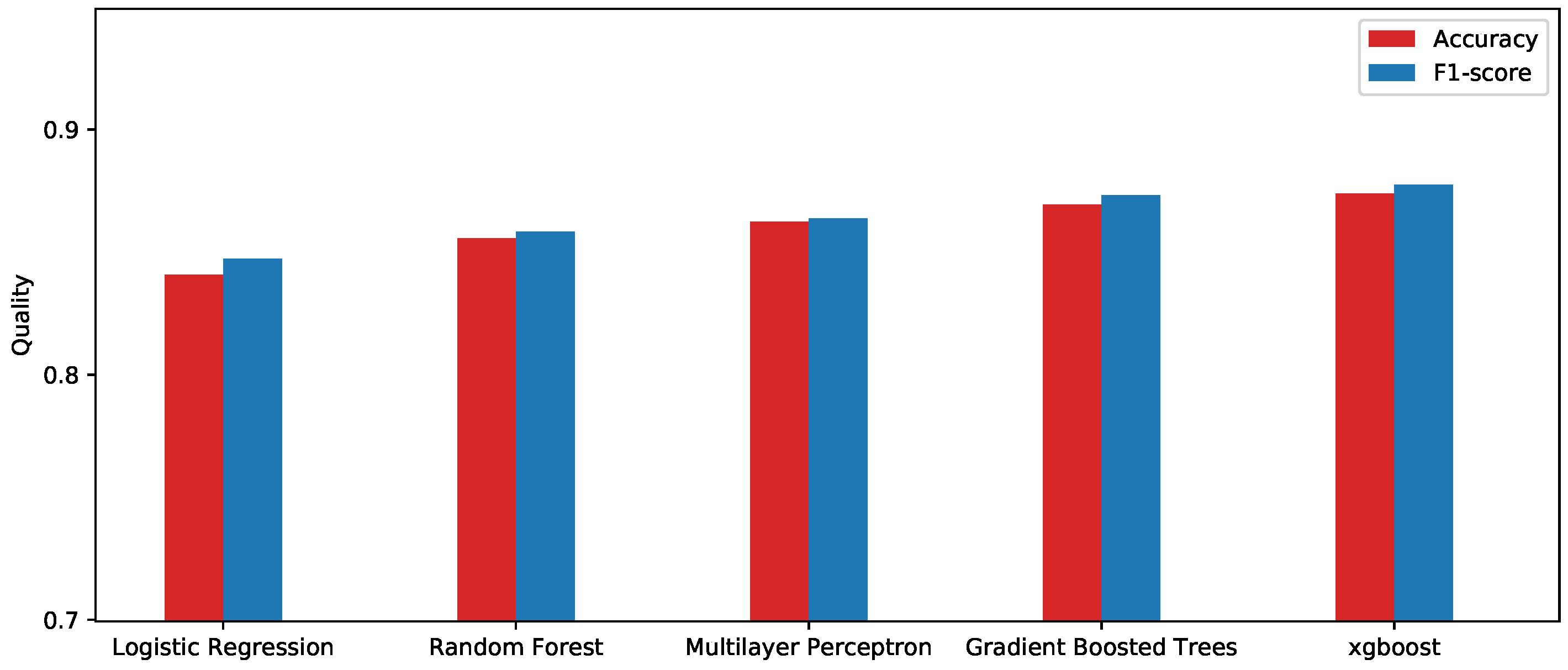
| Method | Accuracy | Precision | Recall | F1-score | Runtime (s) |
|---|---|---|---|---|---|
| Logistic Regression | 0.8407 | 0.8453 | 0.8495 | 0.8474 | 221.3 |
| Random Forest | 0.8555 | 0.8763 | 0.8411 | 0.8584 | 158.1 |
| Multilayer Perceptron | 0.8625 | 0.8915 | 0.8378 | 0.8638 | 16.1 |
| Gradient Boosted Trees | 0.8695 | 0.8836 | 0.8629 | 0.8731 | 425.3 |
| xgboost | 0.8738 | 0.8872 | 0.8679 | 0.8774 | 134.2 |
| Prediction | Correlation | p-Value |
|---|---|---|
| Prediction based on images | 0.0108 | 0.9439 |
| Prediction based on texts | 0.4927 | 0.0006 |
| Prediction based on both images and texts | 0.1063 | 0.4870 |
| Prediction | Correlation | p-Value |
|---|---|---|
| Prediction based on images | 0.8360 | 0.0002 |
| Prediction based on texts | 0.7685 | 0.0013 |
| Prediction based on both images and texts | 0.7208 | 0.0036 |
© 2018 by the authors. Licensee MDPI, Basel, Switzerland. This article is an open access article distributed under the terms and conditions of the Creative Commons Attribution (CC BY) license (http://creativecommons.org/licenses/by/4.0/).
Share and Cite
Feng, Y.; Sester, M. Extraction of Pluvial Flood Relevant Volunteered Geographic Information (VGI) by Deep Learning from User Generated Texts and Photos. ISPRS Int. J. Geo-Inf. 2018, 7, 39. https://0-doi-org.brum.beds.ac.uk/10.3390/ijgi7020039
Feng Y, Sester M. Extraction of Pluvial Flood Relevant Volunteered Geographic Information (VGI) by Deep Learning from User Generated Texts and Photos. ISPRS International Journal of Geo-Information. 2018; 7(2):39. https://0-doi-org.brum.beds.ac.uk/10.3390/ijgi7020039
Chicago/Turabian StyleFeng, Yu, and Monika Sester. 2018. "Extraction of Pluvial Flood Relevant Volunteered Geographic Information (VGI) by Deep Learning from User Generated Texts and Photos" ISPRS International Journal of Geo-Information 7, no. 2: 39. https://0-doi-org.brum.beds.ac.uk/10.3390/ijgi7020039