Measuring the Spatial Relationship Information of Multi-Layered Vector Data


1
School of Remote Sensing and Information Engineering, Wuhan University, Wuhan 430079, China
2
Department of Land Surveying and Geo-Informatics, The Hong Kong Polytechnic University, Hong Kong, China
3
Joint Research Laboratory on Spatial Information, The Hong Kong Polytechnic University, Wuhan University, Hong Kong, China and Wuhan 430079, China
*
Author to whom correspondence should be addressed.
ISPRS Int. J. Geo-Inf. 2018, 7(3), 88; https://0-doi-org.brum.beds.ac.uk/10.3390/ijgi7030088
Submission received: 22 January 2018
/
Revised: 3 March 2018
/
Accepted: 7 March 2018
/
Published: 9 March 2018
Abstract
:Geospatial data is a carrier of information that represents the geography of the real world. Measuring the information contents of geospatial data is always a hot topic in spatial-information science. As the main type of geospatial data, spatial vector data models provide an effective framework for encoding spatial relationships and manipulating spatial data. In particular, the spatial relationship information of vector data is a complicated problem but meaningful to help human beings evaluate the complexity of spatial data and thus guide further analysis. However, existing measures of spatial information usually focus on the ‘disjointed’ relationship in one layer and cannot cover the various spatial relationships within the multi-layered structure of vector data. In this study, a new method is proposed to measure the spatial relationship information of multi-layered vector data. The proposed method focuses on spatial distance and topological relationships and provides quantitative measurements by extending the basic thought of Shannon’s entropy. The influence of any vector feature is modeled by introducing the concept of the energy field, and the energy distribution of one layer is described by an energy map and a weight map. An operational process is also proposed to measure the overall information content. Two experiments are conducted to validate the proposed method. In the experiment with real-life data, the proposed method shows the efficiency of the quantification of spatial relationship information under a multi-layered structure. In another experiment with simulated data, the characteristics and advantages of our method are demonstrated through a comparison with classical measurements.
1. Introduction
With the development of remote-sensing techniques and geographic information science, more detailed geospatial data have become available to represent this real world. However, the increasing complexity of geospatial data because of large volumes and sophisticated content increases the difficulty in conducting spatial reasoning and analysis. We must investigate how complex data are and determine the spatial distribution of the complexity to develop more scientific strategies to process geospatial data. To address this issue, spatial information, which is an effective tool to measure the complexity of geospatial data, has been widely used in both cartography and geographic information systems (GIS) [1]. Geospatial data models can be generally classified into two categories, namely, spatial vector data and raster data, so measurements of their information contents can differ [2]. Raster models contain some unique measurements because these models consist of regular grids with specific values, which permits pixel-related analysis and computation [3,4]. In contrast, spatial features, such as spatial points, lines, and polygons, are used to represent the geographical objects in vector data models. These features are stored in different vector layers according to their geometric types and the properties of their counterparts on the Earth’s surface [5]. The special structure of vector data makes any spatial relationships more complicated [6] and limits comprehensive measurements of their information metrics.
A general classification of spatial information content was proposed by Li and Huang [7], namely, geometric information, spatial relationship (topological) information and thematic information. Geometric information and thematic information mainly concern the shapes and attributes of spatial objects but are beyond the scope of this study and will not be discussed further. Spatial relationship information helps people better understand the relationships between spatial objects [8]. The most commonly used types of spatial relationships include topological relationships, distance relationships, and directional relationships [6]. Sufficient information regarding spatial relationships will benefit how human beings recognize and rationalize spatial situations [9,10]. This study focuses on the quantitative measurement of spatial relationship information.
The concept of entropy was initially proposed by Shannon [11], which later set the cornerstone of information theory [12]. Shannon’s entropy provides a mathematic approach to quantify the diversity of categorical data [13]. Formally, the entropy of a category variable with classes could be written as
where denotes the proportion of objects that belong to the class . The entropy is permanently a positive value and reaches its maximum (i.e., ) when the proportions of all classes are equal (i.e., ). To date, entropy has been widely used for various domains such as regional science, ecology and social science [14,15,16]. Entropy, which is used as a measure of diversity, has been applied to solve problems in geospatial science, such as map efficiency [17,18], spatial heterogeneity [19], spatial clustering [13], scale effects [20], and landscape analysis [21,22].
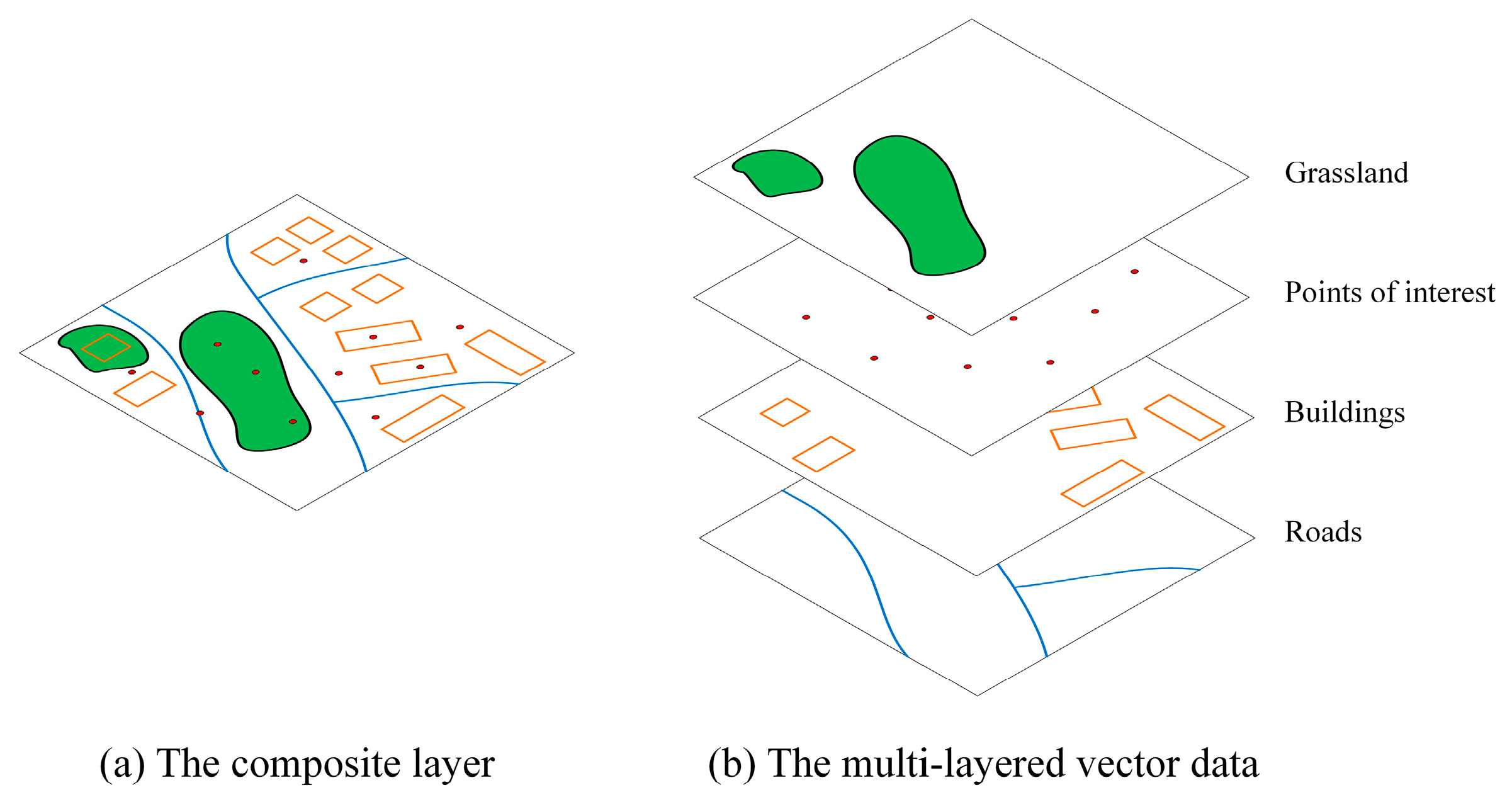
In terms of measuring spatial information content, richer information content is believed to be associated with more complex spatial data [2]. The application of entropy in this field can be traced to the pioneering work of Sukhov [23], who considered the diversity from different types of features on a map. Using the proportion of each type of symbol as , the diversity of a theme map could be simply calculated following Equation (1). Many theoretic models and quantitative measurements of the spatial information content of a map, which is equivalent to the feature diversity, have since been proposed. Neumann [24] performed instructive work on measuring topological information. In his method, vertices are classified according to their neighbor relationships in a graph, which shows all the connections among features in a map, and the entropy is calculated based on the proportions of different types of vertices. Bjørke [25] noted the potential use of information entropy in the automation of map design. Considering the practical goal of a map and the sources of map information, he proposed a set of entropy models to help improve the design of some specific maps, such as dot maps, contour maps and choropleth maps. Li and Huang [7] employed a Voronoi diagram to represent a theme map, and the map information was measured in terms of the distribution of the Voronoi region, neighbors and neighbor types. However, these methods have drawbacks when applied to multi-layered vector datasets. The objects that are measured in these methods are either a single layer or a composite layer, in which all the features are integrated (Figure 1a). In other words, the multi-layered structure of vector data (Figure 1b) is overlooked. Moreover, these measurements mainly focus on the ‘disjointed’ relationship among spatial features, so the effect of other types of spatial relationships among different layers might be underreported. Although some scholars have suggested a solution by processing the evaluations for each layer [26], this operation can only avoid contradictions from overlapping objects, and the essential problem in describing the various spatial relationships among vector layers remains unsolved.
The main purpose of this paper is to provide a solution to quantify spatial relationship information, especially for multi-layered vector data. First, the concept of energy fields is introduced to model the influence of spatial features by analyzing spatial relationships, especially the topological and distance relationships. Then, the information content of any spatial site can be measured by extending Shannon’s entropy. Finally, a particular measurement process and indices of the holistic information content is demonstrated that considers the influence of dense features on spatial relationships.
The remainder of this paper is organized as follows. Some basic models are explained in Section 2. A new method for measuring spatial relationship information and the measurement process are introduced in Section 3. The sensitivity analysis and validation experiments are conducted in Section 4. Finally, the study is discussed and concluded in Section 5.
2. Models
2.1. Energy Field Based on Euclidean Distance
The concept of fields has originated from physics and has been widely applied in geoscience for spatial statistics and analysis [27,28]. In a planar spatial field, any site or location within the space of interest is assigned to a specific value according to its correlations with the spatial objects, which can be viewed as an abstract representation of the influence of spatial objects. In fact, Voronoi diagrams, which have been broadly adopted in earlier studies of spatial-information evaluation [7,29] and spatial-relationship analysis [30,31], have also inherited some basic thoughts of spatial field, that is, dividing the entire area into polygonal partitions, which represent the region that is dominated by a particular spatial object because of its higher degree of closeness than any other object [32]. However, Voronoi diagrams can only reflect the adjacent relationships among features, and the detailed variations in spatial arrangements, such as the relative distance and orientation, are neglected. Although the scale-independent nature of Voronoi diagrams corresponds to topological relationships, these diagrams are inefficient in terms of depicting the distance relationships among spatial objects, which also attaches great importance to reasoning vector data. For these reasons, an energy field is defined based on the Euclidean distance to describe the effect of spatial objects on its surroundings in this study.
The First Law of Geography indicates that closer objects are more related than more distant objects [33]. Therefore, the energy of a specific site is defined as a decreasing function with respect to the shortest distance to the closest spatial feature. Based on the Inverse Distance Weighting (IDW), which is commonly used in spatial interpolation [34,35], is written as a power function:
Differently from Voronoi diagrams, energy fields depend on the scale of the data and thus can reflect the distance relationships and the detailed influence of spatial objects on their surroundings. However, the dimension of distance varies in practice, so the distance unit should be transferred and unified to a specific dimension before further calculation, or the energy values will be completely different and the following measurements will become meaningless. In the following content in this paper, the distance unit, unless otherwise noted, is uniformly set as ‘meter’.
Energy fields are affected by the geometric type of their spatial features. For spatial points and lines, energy fields can be easily generated by calculating the shortest distance and applying the specific energy function, as discussed above. As shown in Figure 2, the energy field of a point appears as a radial circle, whereas that of a line appears as a radial band. However, the calculation process for spatial polygons is different. From the perspective of spatial topological relationships, polygons involve more complicated cases compared to the other two geometric types, such as ‘contains a polygon’, ‘contains a line’, ‘covers a polygon’ and so on [36]. The boundary of a polygon plays an important role in its topological relationships because this boundary is the critical line for the ‘contains’ and ‘disjointed’ cases and is also involved in other relationships such as ‘overlaps’, ‘meets’ and ‘equals’ [37]. In other words, once an object approaches a boundary, its topological relationship with the polygon becomes more uncertain, which might lead to richer information content. Furthermore, the complexity of spatial relationships, which produces information content, relies on the state of knowledge about the data [1]. Therefore, it is generally difficult to judge that whether the interior or exterior of a polygon body are more significant in complicating the spatial relationships, especially when the attributes of features are not considered. So, in this paper, we reasonably take them as the same.
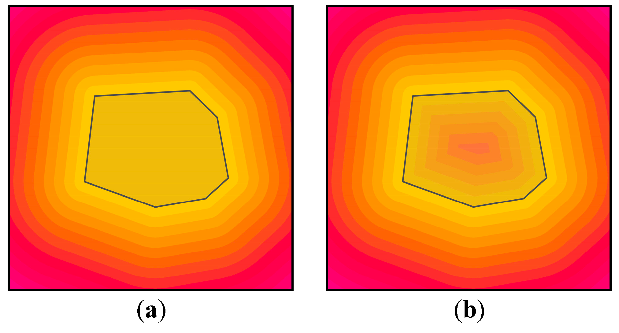
For these reasons, we convert polygon features into line features before computing the energy field. This operation enables us to know the energy changes inside a polygon area. As shown in Figure 3a, the energy field before conversion apparently neglects the energy changes inside the polygon, so all the interior energy is equal. In Figure 3b, areas that are closer to the boundary of the polygon area have more energy, and the interior energy is no longer the same.
2.2. The Information Content of an Energy Set
In this study, the spatial relationships consider the mutual effects among the spatial features from different vector layers, and these mutual effects are reflected by the statistical characteristics of the set of energy values of all sites inside the data’s extent. For a given site, which is always represented by a grid cell in practice, let be the number of layers and be the energy value that is assigned by an energy field of a particular feature of the vector layer. Thus, an energy set can be defined as a combination of energy values from each of the layers and expressed as . Then, the proportion of one energy value on this grid cell can be calculated as follows:
The disorder of an energy set is an essential element when considering its information content. A given grid cell can be regarded as being dominated by specific features when these features exert significantly more energy than the others. In this situation, the spatial relationship information in this grid cell may be derived from these dominant features, and the disorder is lower. Obviously, the less dominant the features, the more diverse the energy set, and thus the greater the spatial information. Therefore, the basic thought of our approach is that an energy set has rich information content if it contains similar energy values. Meanwhile, the amount of information is small if the variation in the energy values is large.
In addition, the absolute value of the energy should be considered in the event an energy set, such as {, has the same entropy (i.e., ) as the set { according to Equation (1). However, the energy set with larger elements should have more information content because the corresponding grid cell is implied to be closer to the spatial features, which attaches more importance to the measurement of distance relationships. For example, a set should have richer information content than { and less than . Moreover, richer information is expected when additional energy is added in a given energy set, so features from more layers are involved in practice. For instance, the information of the set should be larger than that of set . Therefore, we modify the classical entropy formula and define the information content of an energy set as
where is a non-zero positive coefficient with respect to the energy values in the energy set. appears as a discriminant statistic between grid cells, with strong influence on spatial relationships producing a large value and weak influence producing a relatively small value. Similar modifications have been reasoned and applied in previous studies, e.g., measuring the spatial diversity [15].
According to the above discussion, should satisfy the following two criteria.
- Criterion 1, increase monotonically with respect to , mathematically:
- Criterion 2, increase with the number of , that is:
In criteria 1, the derivative of with respect to for all should be larger than zero:
where denotes the sum of an energy set (i.e., ); is the partial differential of with respect to the energy value ; and is the proportion of in the given energy set , which is calculated based on Equation (3).
is defined as a positive value and is not larger than zero for , so the last term in Equation (7), , is constantly greater than or equal to 0. Therefore, the first two terms can be extracted to form the following equation, which can be called an alternative form of Equation (7):
According to the solution of the linear differential equation, the general solution for (8) can be easily computed as follows:
in which is a positive constant. The above equation satisfies Criterion 2 when the constant is set to 1. Therefore, the information content of a given energy set can be written as
, so reaches its maximum value when for all . In other words, when vector objects (points, lines and the boundaries of polygons) appear in the same grid cell for all layers, the grid cell has the richest information content, which can be written as
3. Methods
3.1. Generating the Energy Map and Weight Map
The overall information of a vector dataset can be intuitively calculated by directly summing the information of all the energy sets that are associated with every grid cell inside the extent of the data. Mathematically, this sum method can be expressed as
where denotes the extent of the given dataset, indicates a grid cell with the extent , and refers to the collection of energy sets that are associated with the grid cell .
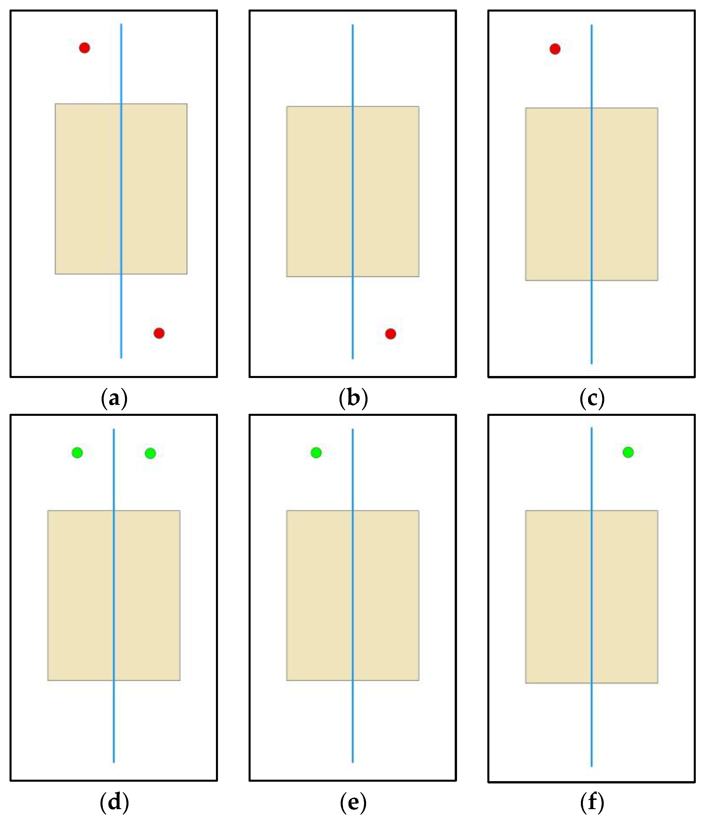
However, the above summation method has two drawbacks. First, according to the definition of energy sets, if features exist in the out of layers, the amount of energy sets in any grid cell can be expected to be , which indicates the number of possible feature pairs across all the layers. The energy field of every feature must be calculated and stored, which will intensively increase the storage and computational cost. Second, the sum function in (12) overlooks that the interactions of the features that belong to the same layer may complicate the spatial relationships. For example, as shown in Figure 4, the information content in (a) could be divided into two components, which equal the information content in (b) and (c). Similarly, the information content in (d) can be called the sum of (e) and (f). Obviously, the information content in (a) and (d) would be the same because the spatial arrangements in (b), (c), (e) and (f) are the same. However, based on our understanding, the spatial relationship in (a) should be more complex than that in (d). The inference is reasonable because the two points in (a) are closer, complicating both the spatial relationship within the point layer and the relationships among multiple layers in the surroundings of these two points.
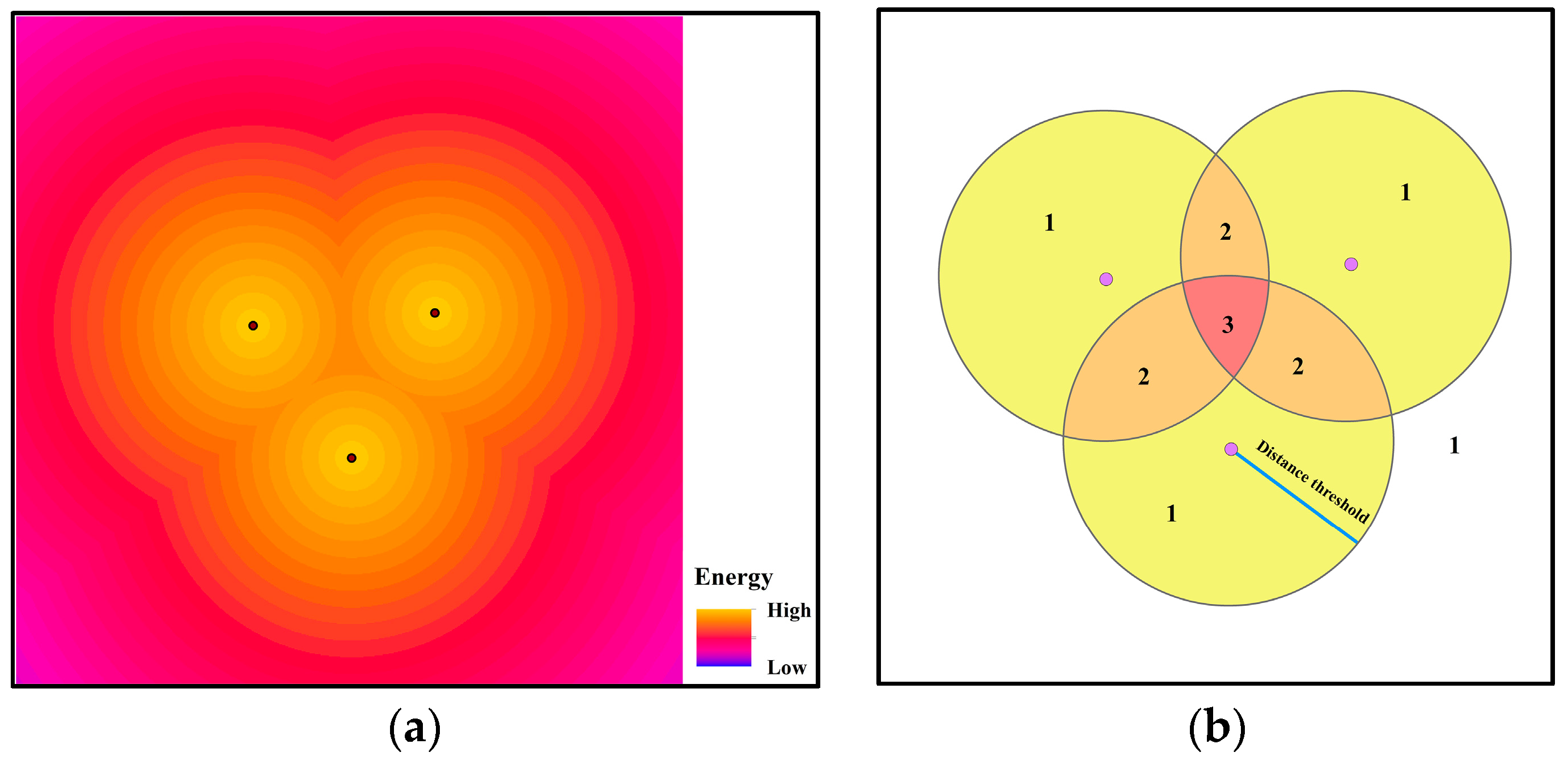
We introduce an energy map and a weight map for each layer in our method to address the abovementioned drawbacks to the direct summation method. In an energy map, each grid cell is assigned the largest energy from the vector features. In fact, this operation aims to avoid the usage of a huge number of energy sets (i.e., , as discussed) in the measurement, and only the largest energy value, which is the main contribution to the spatial relationship information, is saved for further analysis (an example is shown in Figure 5a). On the other hand, a weight map acts as a counter that records the number of features with non-negligible energy on a given grid cell. In practice, this non-negligible influence is incorporated by a distance threshold. Once the distance between the given grid cell and feature is larger than the threshold, the influence of the feature on this grid cell will be ignored (except for the closest feature). Thus, the weight of each grid cell will be counted as the number of features that are no further than the threshold (an example is shown in Figure 5b). This weight map acts as an amplifier for the information contents of jointly affected regions of multiple features within one layer and compensates any information loss from the operation in the energy map (i.e., only the largest energy is recorded and utilized in the measurement).
3.2. Measurement Process
The final information contents can be measured by combining all the energy maps and weight maps in a vector dataset. Here, the process of our method is as follows:
- Set an initial weight for each grid cell in the extent .
- Generate a buffer layer for each vector layer. The buffer size is defined as the longest distance that the influences from features should be considered. The buffer for a polygon is based on the polygon’s boundary, which is consistent with the approach to generate the energy field for a polygon.
- Set , and let denote the buffer layer for the vector layer . Then, divide the extent into areas according to the number of buffers in .
- Let be the number of buffers that cover the area . The weights of the grid cells inside the area are updated: .
- . Return to step 3 until all the buffer layers are traversed.
- Each grid cell will increase by a factor of in terms of their information amounts. Then, the total information is calculated by adding up the information in each grid cell.
Therefore, the total information of a multi-layered vector dataset can be expressed as
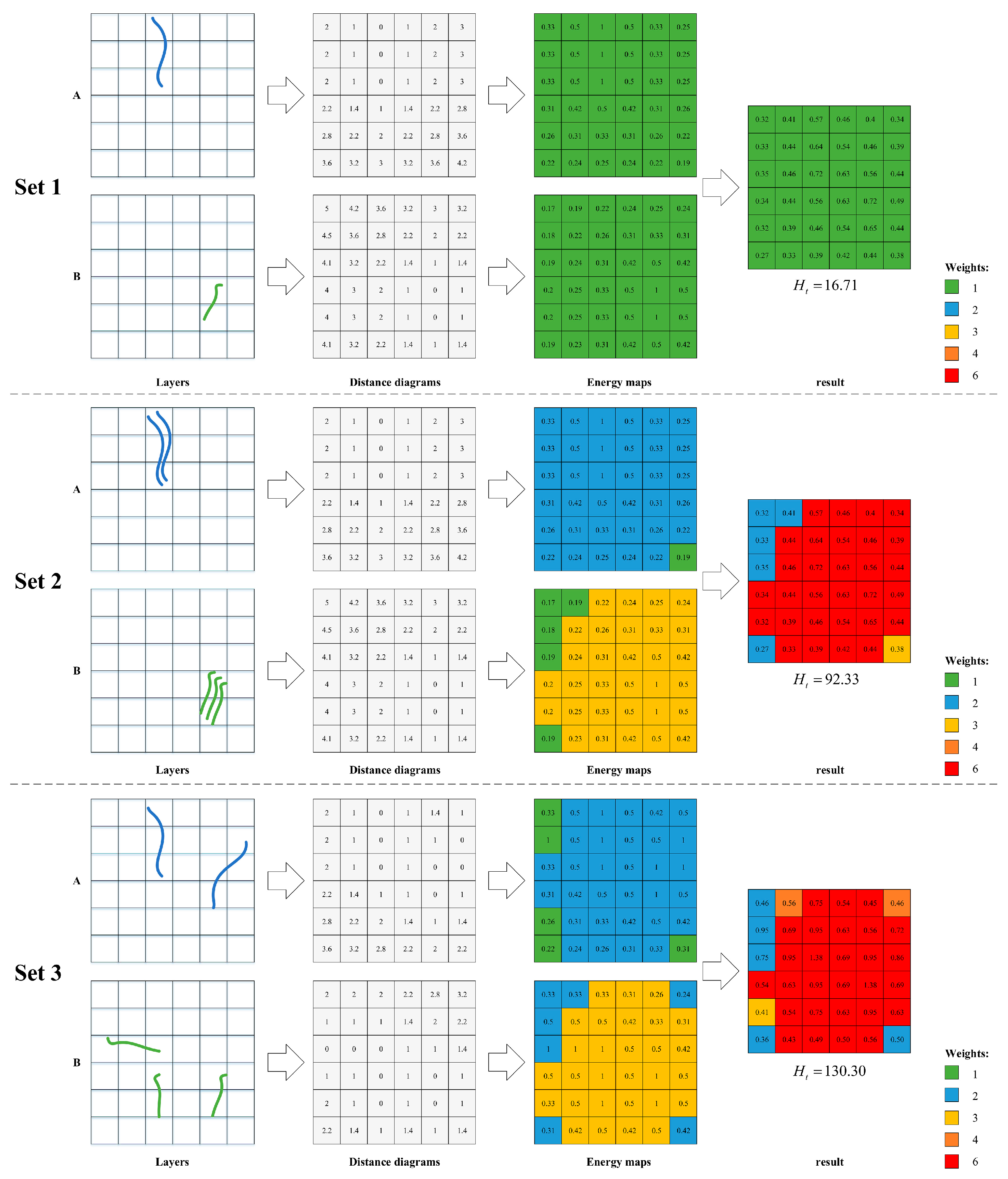
Three sets of simulated data are provided to illustrate the process of our method and validate the rationality of the energy map and weight map. We calculate the Euclidean distance in which the map unit is specified as the height of a given grid size. As shown in Figure 6, the two layers in Set 1 only have one feature. Although more features appear in both layers in Set 2, the energy maps remain the same. The measured information will be the same for Sets 1 and 2 without the augmentations from the weight map. On the other hand, the spatial relationship information is produced by the line pair in Set 1, while six similar line pairs exist in Set 2. Therefore, the spatial relationship information in Set 2 can be expected to be approximately 6 times as much as that in Set 1. Let the buffer size be 4 times the grid height; the final result of our method is 16.71 for Set 2 and 92.33 for Set 1, which is consistent with our expectations and supports the multiplication operation on weights in step 4. Although Set 2 is an extreme case in which all the features in one layer appear at the same location, the feasibility of the measurement process can be extrapolated to a more general case, such as Set 3, in which the features move closer and even intersect, and the spatial relationships become more complicated, producing the larger result of 130.30.
4. Experiments and Analysis
4.1. Sensitivity Analysis of the Grid Size and Buffer Size
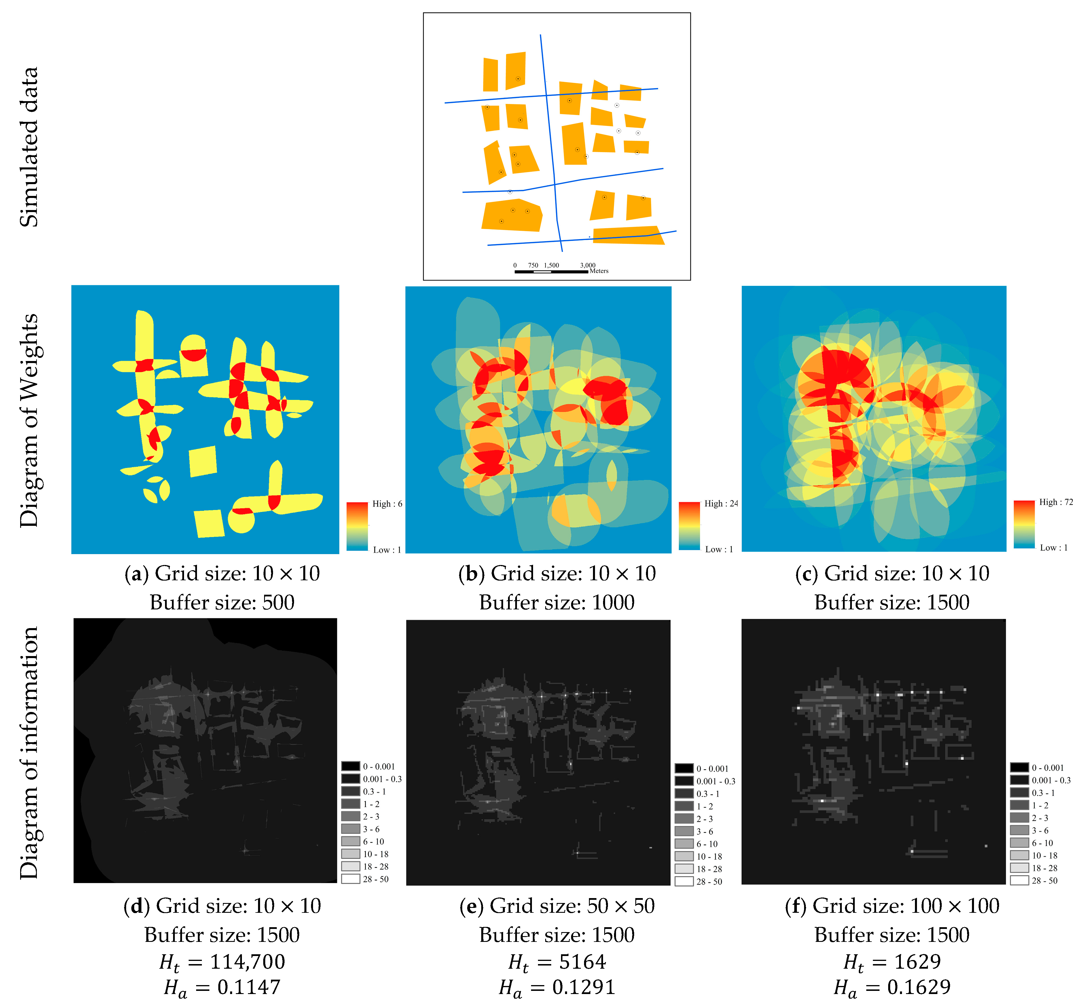
The grid size and buffer size are two critical parameters in our method. To evaluate the effects of these two parameters on the final result, a sensitivity analysis is conducted on a general simulated dataset with three layer-types: polygons, lines, and points. Some basic spatial relationships are designed among these three layers, including ‘contains’, ‘intersects’, and ‘disjointed’. The original data and portions of the intermediate results are shown in Figure 7.
As shown in Figure 7, significant differences exist in the outputs because the grid size and buffer size vary. Figure 7a–c show that larger weights are assigned to a wider range of grid cells as the buffer size increases. This phenomenon is expected because a larger buffer size means that more grid cells will be covered by buffers, and the number of buffers that cover a specific grid may also increase. On the other hand, Figure 7d–f show the diagrams of information gradually becoming coarser as the grid size increases, and the total information dramatically declines (i.e., from 114,700 to 1629). However, according to Equation (13), the total information depends on the number of grid cells (under the same map units), which is determined by the grid size and the total area of the extent . Therefore, only when both the extents and grid sizes are the same for the two datasets can the total information become a comparable index. For this reason, the average information is an alternative, which is defined as
where denotes the number of grid cells within the layer extent .
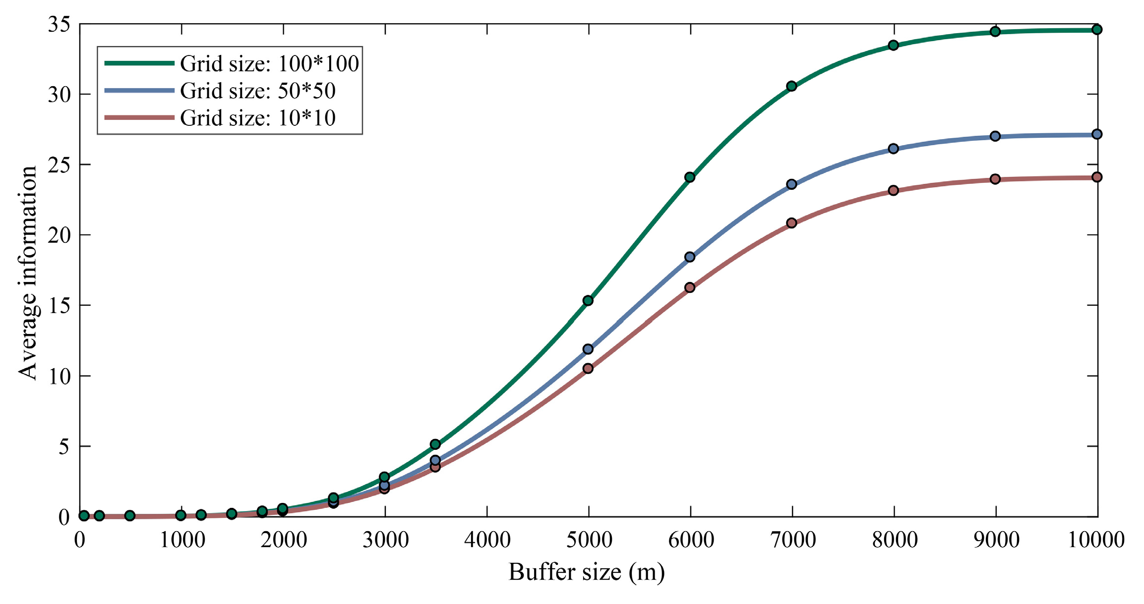
In contrast with the total information, the average information does not rely on the number of grid cells, which makes a comparison between two datasets with different extents possible. After applying the average information, the information contents of the examples from Figure 7d–f are calculated to be 0.1147, 0.1291 and 0.1629, respectively. With different grid sizes, the average information index produces more consistent results than the total information index. Although the variance between the measurements has been significantly narrowed by using the average information index, slight differences still exist, so the comparability of the average information should rely on a uniform grid size. This inference is also supported by the plots in Figure 8. Obviously, the measured information value increases with respect to the buffer size and grid size. This phenomenon suggests that these two parameters should be ascertained and kept consistent in each measurement; otherwise, the measured values will become incomparable and meaningless.
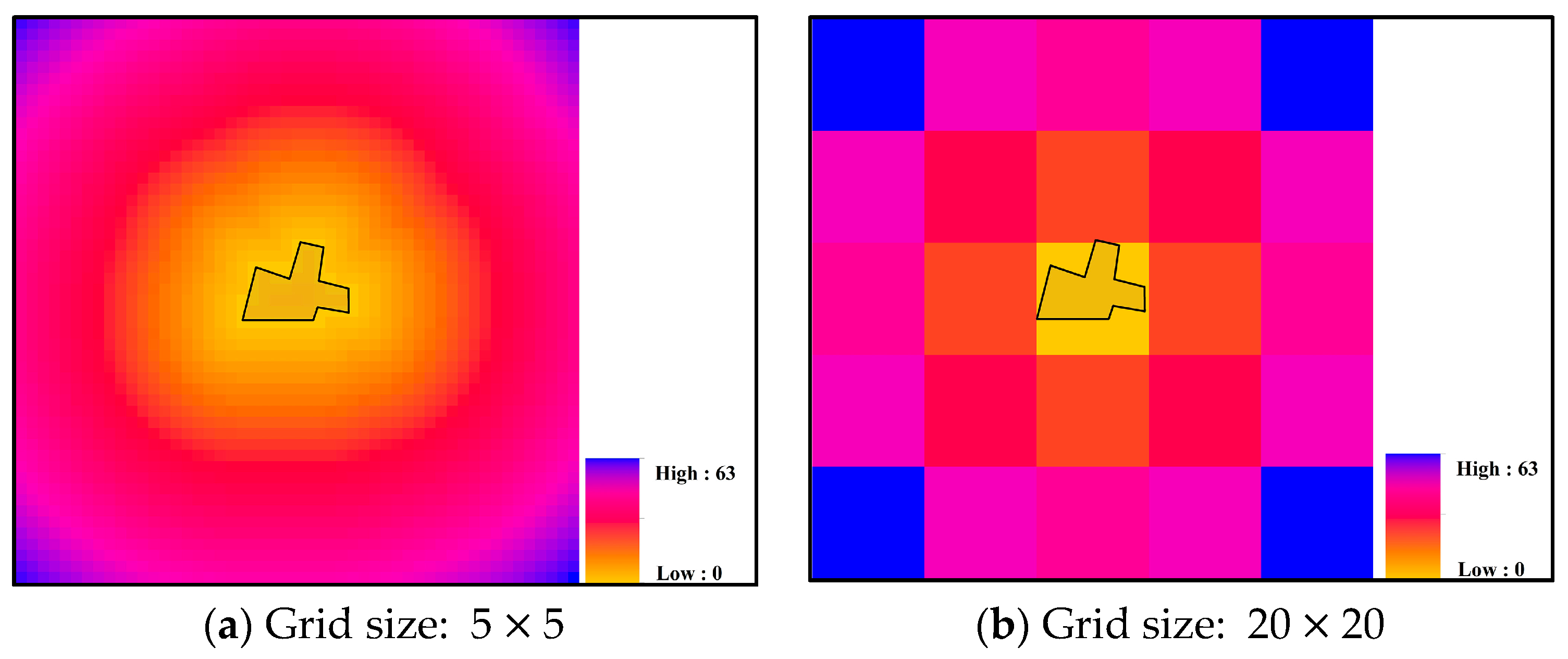
In addition, an inappropriate grid size may introduce uncertainty into the measurement. According to Figure 6d,e,f, the grid size determines the degree of abstraction of the energy map. An intuitive example is illustrated in Figure 9. When a grid cell is larger than the size of a feature (e.g., a line and polygon), the Euclidean distance diagram of this feature is calculated as if the feature has been replaced by one point, and all the shape and size characteristics of the original feature are lost (see Figure 9b). This result may create a very biased input when further modeling the energy map. In this case, the grid size should be defined to be no larger than the smallest minimum bounding square of features within the target dataset; smaller values are preferred if the computational cost is affordable.
4.2. Validation Experiments
In this section, the proposed method is applied to a set of real data for validation. Furthermore, a test is conducted on simulated datasets to compare our method and the classical method by Li and Huang [7] and show the advantages of our method in reflecting the complexity of spatial relationships among multiple layers.
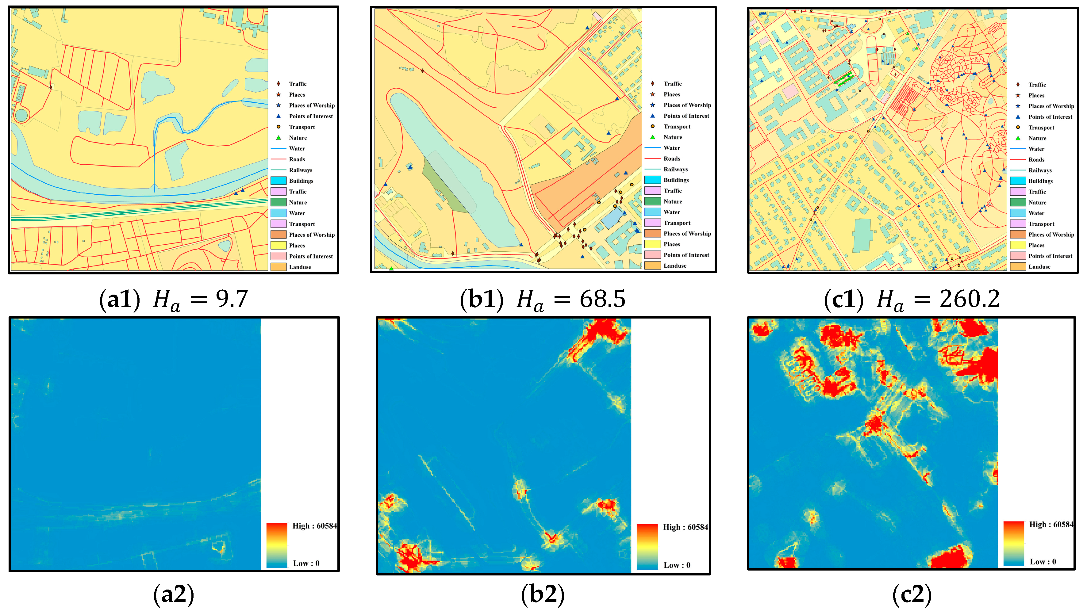
First, we extract three regions of data in Berlin, Germany, as shown in Figure 10, from the global vector data from the collaborative project OpenStreetMap (OSM) (http://download.geofabrik.de/). The experimental dataset has 18 layers, including 7 point-layers, 3 line-layers, and 8 polygon-layers. The details of the layers in these three regions are provided in the Supplementary document. The size of each region is m, while the buffer size and grid size are set to 50 and 5 m, respectively.
As shown in Figure 10, the spatial relationships become more complex from left to right according to visual observation. The statistics of these three datasets (see Table S1 in the Supplementary document) also support this inference because the classes and numbers of spatial features generally increase from (a1)–(c1). The average information of these three regions as calculated by the proposed method is 9.7, 68.5 and 260.2, which is consistent with our inference. On the other hand, the distribution of the spatial relationship information is provided in Figure 10a2,b2,c2. These figures show the regions with high information contents, which might be very useful information in practice. Obviously, our approach can reflect the complexity of these regions of data in terms of spatial relationships.
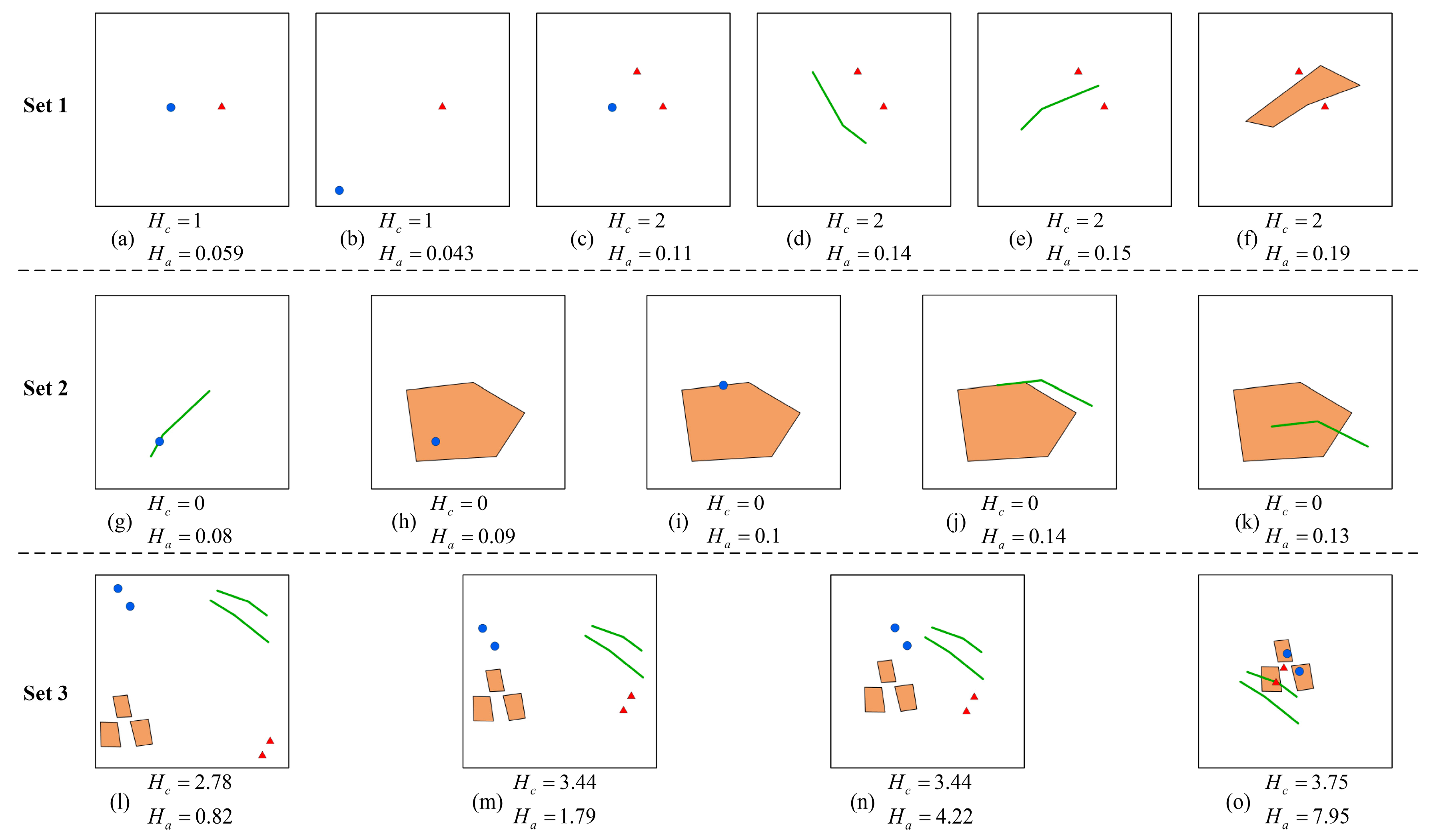
However, one may still question whether the proposed method can capture slight changes in the spatial relationships and has more advantages than the classical method. Therefore, three sets of simulated data, as shown in Figure 11, are used to test the capability of the proposed method. The results of our method and the classical approach by Li and Huang [7] are both calculated for comparison. Li and Huang employed some spatial statistics of Voronoi regions and proposed three types of measurements (i.e., geometric, topological and thematic) to calculate the information of a map [7]. As mentioned in Section 1, our approach focuses on spatial relationship information rather than semantic information, geometric information, etc. Therefore, only the topological information measurements in Li and Huang’s method are calculated and compared in the test.
As shown in Figure 11, Set 1 focuses on the ‘disjointed’ spatial relationship, which is the most common situation in practice. According to the results of this set, our method is more sensitive than the classical method in terms of the relative position ((a), (b) and (d), (e)), feature number ((a) and (c)), and feature type ((c), (e) and (f)). According to the results of Set 2 in Figure 11, the proposed method can distinguish changes in topological relationships, such as ‘contains’ ((g) and (h)), ‘meets’ ((i) and (j)) and ‘overlaps’ (k), while Li and Huang’s method is inefficient in these cases (the measurement is either 0 or 1 for Set 2). More general cases are provided with different types of features (points, lines and polygons) from four layers in Set 3. As the features approach ((l) to (n)) and finally form a relatively complex layout (o), our method’s results adequately reflect the different complexities of these four situations, producing a larger variation than Li and Huang’s method. All these simulated results demonstrate that our method can acceptably distinguishing the complex spatial relationships among multiple layers.
5. Discussion and Conclusions
Our measurement method for spatial relationship information was extended from the basic concept of Shannon’s entropy, although some differences still exist. Shannon’s entropy involves an enclosed system, in which the number of variables is certain and reaches its maximum when each variable has the same possibility. However, in our method, the system consists of a series of energy sets that represent the information of the corresponding grid cells, and the information of a grid cell continues to increase alongside both the absolute energy values and number of energy sets. This difference is reasonable and necessary because most spatial relationship information should originate from regions where the features are dense, which are associated with large energy values. Therefore, our method inherits the ability of entropy to reflect the inner disorder of an energy set and considers additional information content that is produced by large energy values.
The energy function is an essential approach to model the influence of features on their surroundings. In this paper, the energy function was defined as a power function, a reference to the IDW method, which is commonly used in spatial interpolation. In fact, the energy function might not be unique. A power function was chosen because it requires no additional parameters except for the distance value and tends to zero when the distance increases infinitely.
On the other hand, the selection of the grid size and buffer size was crucial to our method. The value of the grid size was suggested to be smaller than the smallest minimum bounding square of the features, which ensured that the shape and size characteristics of all the features could be reflected in the energy map. Meanwhile, the value of the buffer size should be related to the data. During our test on real-life OSM data, a buffer size of approximately 50 m was logical for the following four reasons. First, the buffer size should not be too small, or no buffer will become overlapped and the buffering operation will be meaningless. According to our observations, the average distance between features in one layer in the most feature-dense areas of the OSM data was approximately 30 to 80 m. Second, the energy of a grid cell that is more than 50 m from the nearest feature is less than 0.02 according to Equation (2). This value is thought to be small enough to be ignored. Third, an excessively large buffer size requires very intensive computation, especially for data with a large extent and high feature number. To enhance the efficiency of our method in practical applications, the buffer size should not be excessively large. Finally, the results were satisfactory when the buffer size was set to 50 m in the real-data test in Section 4. In fact, the selection of the buffer size should be ‘suitable’ rather than ‘optimal’ because the relative size of the spatial relationship information in datasets is much more meaningful than the absolute size of the dataset [26]. The measurements are thought to be fair and comparable once the datasets are measured under the same ‘suitable’ buffer size.
In contrast with the classical measure, which always focuses on ‘disjointed’ relationships in one layer, one significant advantage of our method is its sensitivity to the various spatial relationships among multiple vector layers. This advantage enables our method to deal with the complex situations in real-life data, and the results more comprehensively reflect spatial relationships compared to the classical method. Meanwhile, the proposed method emphasizes spatial distance relationships in addition to topological relationships. According to the results of the validation experiments on real OSM data and simulated data, the proposed method can efficiently capture distance changes among features. Furthermore, intermediate products, such as diagram of the information and weights, could provide detailed distributions of the information and intensity of features, which makes the results more understandable.
The proposed method should have wide prospects beyond the traditional applications of spatial information. To our knowledge, the spatial relationships in vector data are closely related to the data quality [38]. Generally, regions with complex spatial relationships are more likely to have quality issues, especially those that are related to logical consistency [38]. By measuring spatial relationship information and analyzing its spatial distribution, one can locate regions with high risk for data-quality issues and then inspect these regions. Spatial relationship information can also provide more details regarding data arrangement and regional differences, which may improve spatial stratification [39] for related spatial analyses and the design of better sampling plans [40] for the acceptance of vector data.
Further work could be performed in the following three aspects. First, efforts should be made to measure the direction relationship information in vector data. Second, the applicability of the current energy function and its alternative formats for different practical requirements should be further studied because of the energy function is not unique. Third, particular raster layers, such as digital elevation models [22], could provide information that may contribute to the spatial relationships, and possible solutions to include raster layers in spatial relationship information metrics should be examined.
Supplementary Materials
The following are available online at https://0-www-mdpi-com.brum.beds.ac.uk/2220-9964/7/3/88/s1. Table S1: Statistics of three experimental regions.
Acknowledgments
This research was supported by the State Key Program of the National Natural Science Foundation of China (No. 41331175), the Innovation and Technology Fund of the Hong Kong Government (No. ITP/053/16LP), and Hong Kong Polytechnic University (1-ZE24, 4-ZZFZ). We are also grateful to the editor and the three referees who provided constructive comments on improving this article.
Author Contributions
Pengfei Chen conceived the presented idea and wrote the manuscript with support from Wenzhong Shi. All the authors have approved the final version of this manuscript.
Conflicts of Interest
The authors declare no conflicts of interest.
References
- Batty, M.; Morphet, R.; Masucci, P.; Stanilov, K. Entropy, complexity, and spatial information. J. Geogr. Syst. 2014, 16, 363–385. [Google Scholar] [CrossRef] [PubMed]
- Fairbairn, D. Measuring Map Complexity. Cartogr. J. 2006, 43, 224–238. [Google Scholar] [CrossRef]
- Stein, A.; De Beurs, K. Complexity metrics to quantify semantic accuracy in segmented Landsat images. Int. J. Remote Sens. 2005, 26, 2937–2951. [Google Scholar] [CrossRef]
- Boots, B. Developing local measures of spatial association for categorical data. J. Geogr. Syst. 2003, 5, 139–160. [Google Scholar] [CrossRef]
- Chang, K.-T. Geographic Information System. Int. Encycl. Geogr. 2017, 1–9. [Google Scholar] [CrossRef]
- Egenhofer, M.J.; Sharma, J. Assessing the consistency of complete and incomplete topological information. Geogr. Syst. 1993, 1, 47–68. [Google Scholar]
- Li, Z.; Huang, P. Quantitative measures for spatial information of maps. Int. J. Geogr. Inf. Sci. 2002, 16, 699–709. [Google Scholar] [CrossRef]
- Renz, J. Qualitative Spatial Reasoning with Topological Information; Springer: Heidelberg, Germany, 2002; Volume 2293, p. 207. [Google Scholar]
- Frank, A.U. Qualitative Spatial Reasoning about Distance and Directions in Geographic Space. J. Vis. Lang. Comput. 1992, 3, 343–373. [Google Scholar] [CrossRef]
- Li, S. Combining topological and directional information for spatial reasoning. IJCAI 2007, 137, 435–440. [Google Scholar] [CrossRef]
- Shannon, C.E. A Mathematical Theory of Communication. Bell Labs Tech. J. 1948, 27, 379–423. [Google Scholar] [CrossRef]
- Shannon, C.E.; Weaver, W. The Mathematical Theory of Communication; University of Illinois Press: Champaign, IL, USA, 1949. [Google Scholar]
- Leibovici, D.G.; Claramunt, C.; Le Guyader, D.; Brosset, D. Local and global spatio-temporal entropy indices based on distance ratios and co-occurences distributions. Int. J. Geogr. Inf. Sci. 2014, 28, 29–41. [Google Scholar] [CrossRef]
- Batty, M. Space, scale, and scaling in entropy maximizing. Geogr. Anal. 2010, 42, 395–421. [Google Scholar] [CrossRef]
- Claramunt, C. A spatial form of diversity. Int. Conf. Spat. Inf. Theory 2005, 3693, 218–231. [Google Scholar] [CrossRef]
- Yu, H.; Winkler, S. Image complexity and spatial information. In Proceedings of the 2013 5th International Workshop on Quality of Multimedia Experience, Klagenfurt am Wörthersee, Austria, 3–5 July 2013; pp. 12–17. [Google Scholar]
- Harrie, L.; Stigmar, H.; Djordjevic, M. Analytical Estimation of Map Readability. ISPRS Int. J. Geoinf. 2015, 4, 418–446. [Google Scholar] [CrossRef]
- Hengl, T.; MacMillan, R.A.; Nikolić, M. Mapping efficiency and information content. Int. J. Appl. Earth Obs. Geoinf. 2013, 22, 127–138. [Google Scholar] [CrossRef]
- Jost, L. Entropy and diversity. Oikos 2006, 113, 363–375. [Google Scholar] [CrossRef]
- Chen, Y.; Sun, K. Information measurement of classification maps and scale effects. In Proceedings of the 2013 IEEE Conference Anthology, Chongqing, China, 1–8 January 2013. [Google Scholar] [CrossRef]
- Gao, P.; Zhang, H.; Li, Z. A hierarchy-based solution to calculate the configurational entropy of landscape gradients. Landsc. Ecol. 2017, 32, 1133–1146. [Google Scholar] [CrossRef]
- Hu, L.; He, Z.; Liu, J.; Zheng, C. Method for measuring the information content of terrain from digital elevation models. Entropy 2015, 17, 7021–7051. [Google Scholar] [CrossRef]
- Sukhov, V. Information capacity of a map entropy. Geod. Aerophotogr. 1967, 10, 212–215. [Google Scholar]
- Neumann, J. The Topological Information Content of a Map An Attempt at a Rehabilitation of Information Theory in Cartography. Int. J. Geogr. Inf. Geovis. 1994, 31, 26–34. [Google Scholar] [CrossRef]
- Bjørke, J.T. Framework for entropy-based map evaluation. Cartogr. Geogr. Inf. Sci. 1996, 23, 78–95. [Google Scholar] [CrossRef]
- Wang, S.; Wang, Z.; Du, Q. A measurement method of geometrical information considering multi-level map feature. Sci. Surv. Mapp. 2007, 32, 60–62. [Google Scholar]
- Wolpert, R.; Ickstadt, K. Poisson/gamma random field models for spatial statistics. Biometrika 1998, 85, 251–267. [Google Scholar] [CrossRef]
- Mai, P.M.; Beroza, G.C. A spatial random field model to characterize complexity in earthquake slip. J. Geophys. Res. Solid Earth 2002, 107, ESE 10-1–ESE 10-21. [Google Scholar] [CrossRef]
- Liu, X.; Wu, J.; Xu, J. Characterizing the risk assessment of heavy metals and sampling uncertainty analysis in paddy field by geostatistics and GIS. Environ. Pollut. 2006, 141, 257–264. [Google Scholar] [CrossRef] [PubMed]
- Chen, J.; Zhao, R.; Li, Z. Voronoi-based k-order neighbour relations for spatial analysis. ISPRS J. Photogramm. Remote Sens. 2004, 59, 60–72. [Google Scholar] [CrossRef]
- Long, Z.; Li, S. A complete classification of spatial relations using the Voronoi-based nine-intersection model. Int. J. Geogr. Inf. Sci. 2013, 27, 2006–2025. [Google Scholar] [CrossRef]
- Drysdale, R.L. Generalization of Voronoi Diagram In the plane. SIAM J. Comput. 1981, 10, 73–87. [Google Scholar]
- Tobler, W.R. A Computer Movie Simulating Urban Growth in the Detroit Region. Econ. Geogr. 1970, 46, 234. [Google Scholar] [CrossRef]
- Bartier, P.M.; Keller, C.P. Multivariate interpolation to incorporate thematic surface data using inverse distance weighting (IDW). Comput. Geosci. 1996, 22, 795–799. [Google Scholar] [CrossRef]
- Baczkowski, A.J.; Clark, I. Practical Geostatistics. J. R. Stat. Soc. Ser. A 1981, 144, 537. [Google Scholar] [CrossRef]
- Chen, J.; Li, C.; Li, Z.; Gold, C. A voronoi-based 9-intersection model for spatial relations. Int. J. Geogr. Inf. Sci. 2001, 15, 201–220. [Google Scholar] [CrossRef]
- Egenhofer, M.J.; Sharma, J. Topological relations between regions in ρ2 and Z2. In International Symposium on Spatial Databases; Springer: Berlin/Heidelberg, Germany, 1993; pp. 316–336. [Google Scholar]
- Guptill, S.C.; Morrison, J.L. Elements of Spatial Data Quality; Elsevier: Amsterdam, The Netherlands, 2013; Volume 1, ISBN 1483287947. [Google Scholar]
- Wang, J.-F.; Stein, A.; Gao, B.-B.; Ge, Y. A review of spatial sampling. Spat. Stat. 2012, 2, 1–14. [Google Scholar] [CrossRef]
- Tong, X.; Wang, Z.; Xie, H.; Liang, D.; Jiang, Z.; Li, J.; Li, J. Designing a two-rank acceptance sampling plan for quality inspection of geospatial data products. Comput. Geosci. 2011, 37, 1570–1583. [Google Scholar] [CrossRef]
Figure 1.
Examples of a composite layer and multi-layered vector data.

Figure 2.
(a) Energy field for a point; (b) energy field for a line.

Figure 3.
(a) Energy field for a polygon before conversion; (b) energy field for a polygon after conversion.
Figure 3.
(a) Energy field for a polygon before conversion; (b) energy field for a polygon after conversion.

Figure 4.
Example of the drawbacks of the direct summation method. The points, lines and polygons represent different spatial features. (a,d) have different spatial relation information since the points are much closer in (d). (b,c,e,f) have the same spatial relationship information because they can be mutually transferred by rotation or symmetry.

Figure 5.
Examples of an energy map (a) and weight map (b). The points in (a,b) denote the spatial point features. In (a), every grid cell is assigned the largest energy value from the features. In (b), the distance threshold equals the length of the blue line, and weights are assigned and labeled in different regions according to the number of overlaps. The region outside of the circles also has a weight value of 1.

Figure 6.
Three examples of the measurement process. The feature distributions of the layers are shown in the first column. The Euclidean distance diagram is illustrated in the second column. The energy maps and final information results are demonstrated in the last two columns. Weights are described by different colors in the grid cells of the energy maps. The weights in the results are calculated by multiplying the weights of the corresponding grid cells in the energy maps in accordance with step 4 in the proposed procedure.

Figure 7.
Simulated data and some intermediate results of the sensitivity analysis. The extent of this simulated data is 10,000 10,000 m. The effect of the buffer size is roughly revealed from (a–c) by fixing the grid size and gradually increasing the buffer size. The effect of the grid size is shown from (d–f), in which the buffer size remains consistent. denotes the total information and denotes the average information.

Figure 8.
Plots of the average information with different buffer sizes and grid sizes.

Figure 9.
Euclidean distance diagrams with different grid sizes. After applying a small grid size (i.e., ) in (a), the diagram reflects the shape and size characteristics of the feature, whereas all the characteristics are lost in (b), which has a larger grid size (i.e., ).
Figure 9.
Euclidean distance diagrams with different grid sizes. After applying a small grid size (i.e., ) in (a), the diagram reflects the shape and size characteristics of the feature, whereas all the characteristics are lost in (b), which has a larger grid size (i.e., ).

Figure 10.
Three regions of real data and the corresponding information distributions. The buffer size and grid size are set to 50 and 5 m, respectively. The original data with increasing degree of complexity (through visual observation) are shown in (a1), (b1) and (c1). The corresponding information distributions are mapped in (a2), (b2) and (c2).

Figure 11.
Tests on three sets of simulated data. denotes the average information as measured by our method, and is the measurement of topological information in Li and Huang’s approach. The extent is 100 100 m, and the grid and buffer sizes are set to 1 and 50 m, respectively. Layers are rendered with different colors. Set 1 analyzes the sensitivity to the feature number, feature type, and relative position. Set 2 tests the capability to distinguish topological changes. Set 3 tests the efficiency in more generally complex situations.

© 2018 by the authors. Licensee MDPI, Basel, Switzerland. This article is an open access article distributed under the terms and conditions of the Creative Commons Attribution (CC BY) license (http://creativecommons.org/licenses/by/4.0/).
Share and Cite
MDPI and ACS Style
Chen, P.; Shi, W. Measuring the Spatial Relationship Information of Multi-Layered Vector Data. ISPRS Int. J. Geo-Inf. 2018, 7, 88. https://0-doi-org.brum.beds.ac.uk/10.3390/ijgi7030088
AMA Style
Chen P, Shi W. Measuring the Spatial Relationship Information of Multi-Layered Vector Data. ISPRS International Journal of Geo-Information. 2018; 7(3):88. https://0-doi-org.brum.beds.ac.uk/10.3390/ijgi7030088
Chicago/Turabian StyleChen, Pengfei, and Wenzhong Shi. 2018. "Measuring the Spatial Relationship Information of Multi-Layered Vector Data" ISPRS International Journal of Geo-Information 7, no. 3: 88. https://0-doi-org.brum.beds.ac.uk/10.3390/ijgi7030088
Note that from the first issue of 2016, this journal uses article numbers instead of page numbers. See further details here.