Article

Accuracy Assessment of Point Clouds from LiDAR and Dense Image Matching Acquired Using the UAV Platform for DTM Creation

Department of Photogrammetry, Remote Sensing and Spatial Information Systems, Faculty of Geodesy and Cartography, Warsaw University of Technology, Plac Politechniki 1, 00-661 Warsaw, Poland
*
Author to whom correspondence should be addressed.
ISPRS Int. J. Geo-Inf. 2018, 7(9), 342; https://0-doi-org.brum.beds.ac.uk/10.3390/ijgi7090342
Submission received: 16 July 2018 / Revised: 3 August 2018 / Accepted: 20 August 2018 / Published: 23 August 2018
(This article belongs to the Special Issue Leading Progress in Digital Terrain Analysis and Modeling)

Abstract

:
In this paper, the results of an experiment about the vertical accuracy of generated digital terrain models were assessed. The created models were based on two techniques: LiDAR and photogrammetry. The data were acquired using an ultralight laser scanner, which was dedicated to Unmanned Aerial Vehicle (UAV) platforms that provide very dense point clouds (180 points per square meter), and an RGB digital camera that collects data at very high resolution (a ground sampling distance of 2 cm). The vertical error of the digital terrain models (DTMs) was evaluated based on the surveying data measured in the field and compared to airborne laser scanning collected with a manned plane. The data were acquired in summer during a corridor flight mission over levees and their surroundings, where various types of land cover were observed. The experiment results showed unequivocally, that the terrain models obtained using LiDAR technology were more accurate. An attempt to assess the accuracy and possibilities of penetration of the point cloud from the image-based approach, whilst referring to various types of land cover, was conducted based on Real Time Kinematic Global Navigation Satellite System (GNSS-RTK) measurements and was compared to archival airborne laser scanning data. The vertical accuracy of DTM was evaluated for uncovered and vegetation areas separately, providing information about the influence of the vegetation height on the results of the bare ground extraction and DTM generation. In uncovered and low vegetation areas (0–20 cm), the vertical accuracies of digital terrain models generated from different data sources were quite similar: for the UAV Laser Scanning (ULS) data, the RMSE was 0.11 m, and for the image-based data collected using the UAV platform, it was 0.14 m, whereas for medium vegetation (higher than 60 cm), the RMSE from these two data sources were 0.11 m and 0.36 m, respectively. A decrease in the accuracy of 0.10 m, for every 20 cm of vegetation height, was observed for photogrammetric data; and such a dependency was not noticed in the case of models created from the ULS data.

Graphical Abstract

1. Introduction

The subject of accuracy comparison of two leading airborne data sources, airborne laser scanning (ALS) and photogrammetric image-matching, has been discussed in several References [1,2,3]. Such a discussion is also present in a comparison of close-range datasets, i.e., terrestrial laser scanning data was compared with the Structure-from-Motion technique in many applications [4,5,6,7]. The accuracy of the Digital Terrain Model (DTM) is crucial for applications related to hydrology and safety. It was proved that the accuracy of the model influences the hydraulic modelling results, and flood hazard area detection [8]. Using optical data in this issue has rapidly grown after the development of the Dense Image Matching (DIM) algorithm [9,10,11,12].
Over the past decade, there was a significant development in photogrammetric techniques based on images from Unmanned Aerial Vehicles (UAVs), for generating digital elevation models, including surface models and filtered digital terrain models [13]. UAV photogrammetry can also be used in archaeology, for generating high-resolution and scaled 3D models of complex sites [14], and in monitoring, for example, monitoring coastal areas [15]. The DTM can be used for levee monitoring, which is related to the data tested in this paper. Through comparison of the DTMs that are acquired in different seasons, it is possible to examine if some damage to the levee structures has occurred, and as a result, to prevent a flooding hazard. Structure-from-motion algorithms deliver point clouds, which are characterized by a high spatial resolution. The largest disadvantage of point clouds achieved from photogrammetry is the vegetation influence, decreasing the vertical accuracy of the derived digital terrain model [16,17]. Many filtering algorithms for point cloud filtering can be tested [18], to eliminate the influence of both high vegetation [19] and low vegetation [20]. However, not every mission will be influenced by the vegetation. For example, when mapping bare earth areas, such as mine sites, earthwork projects or other plane areas [21,22], UAV photogrammetry is a cost effective and accurate technique to use. In cases where the DTM is not significantly important and the only product to assess is the Digital Surface Model (DSM), UAV photogrammetry can provide accuracies better than 0.10 m [15,23,24,25], even with compact cameras.
Ultralight laser scanners, which can be mounted on UAVs, have been developed in recent years [26]. They can provide elevation data, not influenced much by vegetation, and they deliver initial data to digital terrain models that describe the bare ground in an accurate manner. A gradual development of UAV laser scanning (ULS) technology can be observed on the global market [27,28]. The important part of a ULS system is the navigation unit, i.e., integrated Global Navigation Satellite System with Inertial Measurement Unit (GNSS/IMU). To provide the best results for the point cloud, an accurate distance measurement (laser) and the external orientation parameters of a platform are needed. Moreover, a fast-developing, light and reliable GNSS/IMU market can help to provide effective and useful ultralight laser scanning systems. An increasing number of turnkey solutions are offered by major ULS manufacturers (e.g., Riegl, YellowScan, LidarSwiss, Phoenix, LidarUSA, Sabre Sky-3D, Routescene), which enable users to obtain accuracy that is comparable to airborne laser scanning, and close to direct surveying measurements in the field. ULS is a suitable technology when mapping narrow corridor objects, such as levees, which were investigated in this experiment. The most important problems with high-tech scanners and advanced navigation units are the purchase costs, potential losses, and despite developing miniaturization, the weight of this type of sensor. This issue implies that not every task related to the generation of an elevation model requires the use of a laser scanning system. When the accuracy of the DIM is sufficient and the circumstances of the flying mission are appropriate, photogrammetry with UAV images could be a better solution. While favorable circumstances of flight missions are understood as conducted after the end of vegetation season or just after mowing the grass that covers the levees, in this example of an area (mowing is performed even several times per year), what is directly related to vegetation height has an influence on the DIM results. Investigation in this research compares the results of the DTM accuracy for different data sources, helping to provide an answer to this issue.
In this paper, we conducted an experiment on the vertical accuracy of the generated digital terrain models, from two data sources from the UAV platform in extreme resolution. The results also referred to the land cover of the vegetation, which has a crucial influence on the accuracy to investigate which remote sensing data can be used for the DTM generation. The impact of the resolution was also checked in the tests. After the introduction, in the second section, the collected data, test area, and methodology of the experiment are described. The third section presents the results of a comparison of the digital terrain models from the ULS data and DIM point clouds, to the GNSS-RTK surveying measurements, and a comparison with the DTM from the archival airborne laser scanning. It is worthwhile to note that in all analysis, various land cover described by different heights of vegetation is considered to help define which technology is more suitable for the selected area. The obtained results are discussed and used to draw conclusions in the final part of the paper. The significance of the issues presented in this paper are related to the performance capabilities of the accuracy level of the dedicated UAV, with a very high-resolution scanning sensor, compared with a commonly used low-altitude photogrammetric approach for DTM generation. This considers modern trends in sensor development and the growing resolution of remote sensing data.

2. Materials and Methods

2.1. Experiment Description

The main goal of this experiment was to assess the vertical accuracy of DTM from LiDAR and DIM point clouds acquired with a UAV platform. The evaluation of accuracy on areas covered with vegetation was tested, and information about the accuracy of both techniques on different vegetation heights is provided. The test compared both technologies and referred to the growing season, when the accuracy of the image-based approach could be worse than the LiDAR technique. After this season, when the vegetation influence was lower, the results for both techniques could be more similar for the uncovered areas. It could also be tested in experiments using sensors that provide extremely high-resolution data, reaching a few hundred points per square meter. The effect of the experiment showed information about the possibilities of using both approaches when considering data from UAV platforms: ULS and low-altitude photogrammetry with DIM.

2.2. Platform

In the experiment, one platform was used to collect data in the test area (see Figure 1). The Hawk Moth was equipped with two remote sensing sensors. Its specifications are presented in Table 1. The first, is the ultralight laser scanning system YellowScan Surveyor, which is one of the lightest LiDAR solutions on the market dedicated to low-altitude airborne platforms. Its weight was approximately 1.6 kg (battery included). According to the producer, a georeferenced point cloud data collected with the YellowScan Surveyor should be characterized by sub-decimetric accuracy. The Applanix APX15 single board GNSS-Inertial solution, which was a component of this scanner, plays a key role in ensuring the expected accuracy [29]. This sensor used the Velodyne laser sensor (VLP-16), and it is one of the newest laser systems on the market compared to others. A list of UAV-dedicated laser scanners can be found in the example, in References [27,28]. The second sensor, is the RGB compact camera Sony Alpha a6000, which is a very common tool used in photogrammetric projects where UAVs are used. Its APS-C CMOS sensor was 24.3 MPix in resolution. A Sony E-Mount 16 mm with F/2.8 lens, was used in this experiment.

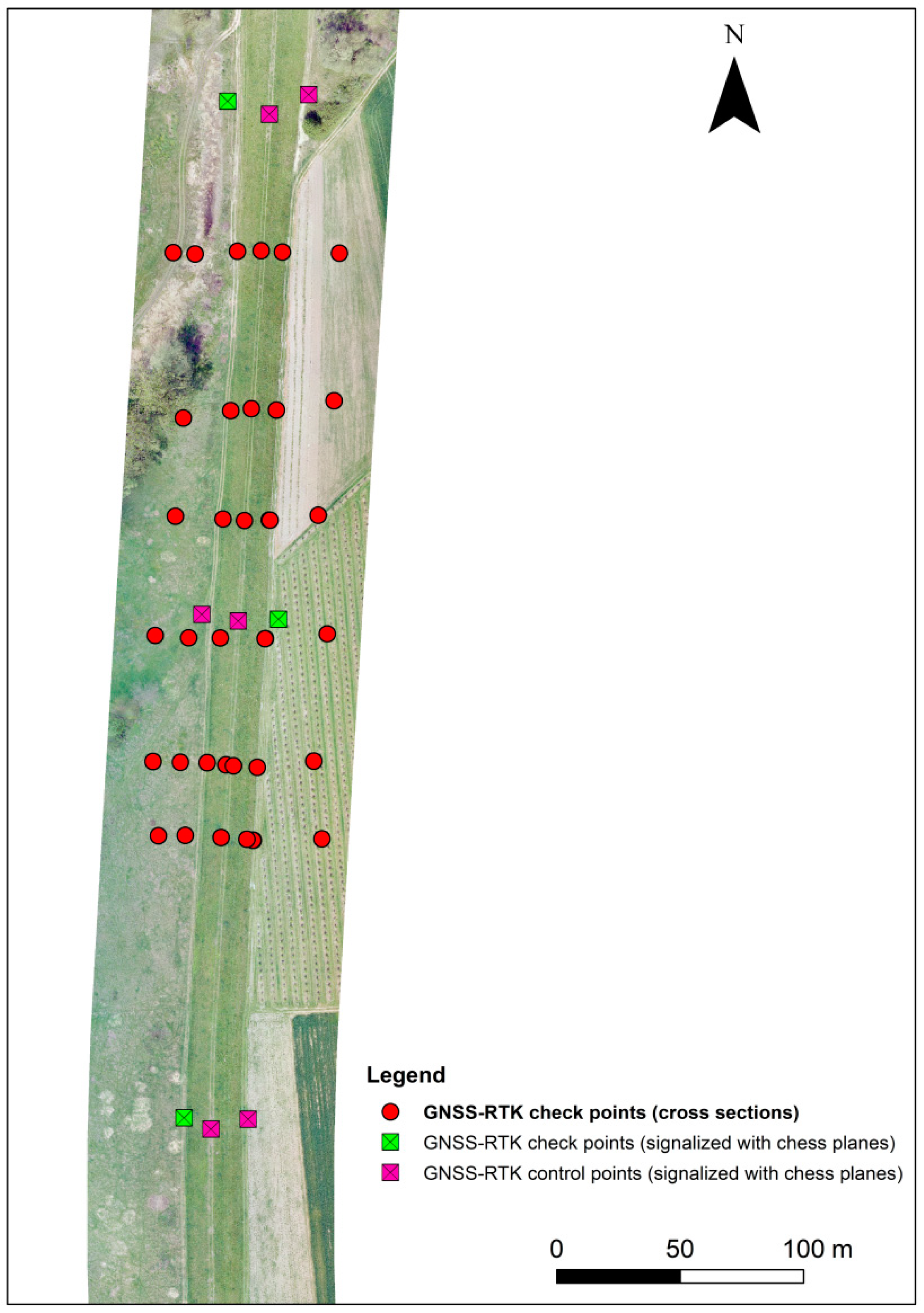
2.3. Test Area and Data Used in the Experiment

The test area was located in the Święciechowska Valley, near the city of Annopol, Lubelskie Voivodeship, Poland (see Figure 2). It contained 6.3 km of levees on the east side of the Vistula river. The test area was covered by high mixed vegetation, agricultural plants, roads, bushes, and trees. The type and height of the vegetation were also different.
The data used in the experiment were acquired on 15–16 May 2017, at an altitude of 50 m above the test area (approximately 48 m above the levee crown), within the inventory of the levee. The length of the laser strips depended on the levee shape (straight flight trajectory preferred, see example in Figure 3), and on the battery life. Eight flight missions were conducted over the test area. The methodology of the performed flights was based on experience with a platform which was equipped with similar sensors, and the processing of data obtained from that platform [30,31]. The mission over the levees was conducted using two strips, with an overlap of 50% for sidelap and 70% for endlap; the control points were signalized with chess planes in the size of 0.5 × 0.5 m and placed regularly on the area to be used during orientation and evaluation, of both LiDAR data and digital images. This configuration of the signalized points was used to improve the absolute elevation accuracy on the mapped levee. Both the control and check points were placed horizontally next to each other, but the Z-coordinates were different, up to several meters (i.e., the levee height). The points were placed on the top and on both sides of the levee. In each cross-section, there were three points measured. One of them was always the checkpoint, and two of them guaranteed that in a case of gross error, we had some redundant observation. The upper part of the area was outside of the test study, and therefore, no check points were distributed there. However, the UAV was registering the data there, and thus, they were included in Figure 3. The additional cross-sections of the terrain were also collected to check the accuracy of the final product of the DTM. These cross sections, measured with GNSS-RTK, were the independent observations without point signalizing. This approach can be used as a valuable assessment of DTM accuracy, because this method is the typical method for levee inventory.
The point cloud from the UAV laser scanning (see Figure 4a) was characterized by a density of 180 points per square meter. Multiple returns have been registered in the point cloud. The first returned laser pulses were approximately 99% of the whole point cloud, and the second only 1%. The mean value of sigma0 in the point cloud (the standard deviation of the interpolated height for each point to the planes, calculated in the algorithm described in Reference [32]), for uncovered areas was 0.02 m, which was related to the size of the noise in the data. The orientation of the LiDAR data was processed in the Applanix software (PosPack), using reference stations from the Active Geodetic Network EUPOS (ASG EUPOS), to adjust the trajectory of the platform with the included parameters of bore-sight calibration angles from the manufacturer and the defined lever-arm parameters. The accuracy of trajectory adjustment, which is a crucial part of the data processing for final accuracy [33], was processed in PosPack and was 0.02 m. This accuracy was reached using the Applanix SmartBase module, which allowed processing of the raw GNSS observations from a network of 4 to 50 reference stations, to compute the atmospheric, clock, and orbital errors within the network. In this case, there were 5 reference stations with baseline lengths from 10 to 50 km. The scanning system used in the experiment was equipped with a single GNSS antenna, initialized on the ground before take-off. The next task was to filter out point clouds and extract bare ground points. This step was processed in Terrasolid software, using Axelsson’s algorithm [34]. The parameters of the ground filtering were set during the testing of the data sample, and the final results of the filtering were obtained when the maximum terrain angle was 80 degrees, the maximum iteration angle was 6 degrees, and the maximum iteration distance was 2 m. During the selection of the filtering settings of the slopes in the terrain, the point cloud density and the size of the gaps in the point cloud had an influence on this decision. The results of filtering were verified in cross sections of point clouds and were manually corrected.
Referring to photogrammetric data, 1285 images with a Ground Sampling Distance (GSD) of 2 cm, collected with the RGB camera with a 70/50 overlap, were oriented in Agisoft Photoscan 1.2.6, based on the control points measured with GNSS-RTK, as signalized in each flight mission, which divided the test area into 8 sections. Each section was adjusted separately. The bundle adjustment with a self-calibration process was performed using ground control points and the images’ position provided by drone navigation sensors. The average accuracy for 73 control points during the bundle adjustment was RMSX = 0.066 m, RMSY = 0.060 m, and RMSZ = 0.084 m, and for 35 check points was RMSX = 0.061 m, RMSY = 0.063 m, and RMSZ = 0.068 m. Another 193 check points not signalized with planes were used within the evaluation of the digital terrain models. Detailed results of the bundle adjustment, can be found in Table 2.
Oriented images were used to generate the point cloud in Agisoft Photoscan, and its density was approximately 1700 points per square meter. Image-based point clouds were filtered to remove the points that represent the land cover (see Figure 4b). Agisoft has a tool to automatically classify the point cloud into “ground” and “non-ground” classes, which also uses Axelsson’s filtering algorithm. In this study, the following parameters were set: maximum angle of 35 degrees not to exclude the points on sloped levees, maximum distance of 1 m and cell size of 50 m, which considered large areas covered by vegetation without ground points.
Comparing the two views of point clouds from two data sources in Figure 4, the higher density of the image-based point cloud is noticed first. It is also worthwhile to mention that the lack of points in the photogrammetric point cloud is not the result of point cloud filtering, but the result of matching algorithm failure in vegetated areas. Processing these two datasets provided the possibility of generating digital terrain models, which were the final product of all the point cloud processing. In the case of the DIM point cloud, approximately 95% of the points were assigned to ground class, which was caused by the lack of points matched on the ground truth, covered by vegetation. During filtering, the points of low vegetation in large areas were often assigned to the ground class; however, buildings, trees, and other surface objects were successfully filtrated. In contrast to the classification of the DIM point cloud, in dense ULS point clouds, only 5% of the points were classified as bare ground. In this case, in a point cloud, there are many returns, and the extraction of ground points provides different filtering statistics compared to the image-based approach.
The main reference data were 193 check points, measured in 18 profiles using the GNSS-RTK technology (Figure 5). Such cross sections on levees, are a typical surveying measurement, which is collected every few years to control the condition of this infrastructure against flooding. In this research, these points were used to evaluate the accuracy of the tested technologies in the case measurements, whilst referring to bare ground (the accuracy of DTM). The accuracy of GNSS-RTK measurements in this case, was assumed to be 0.02 m.
Additionally, the ULS data were also compared to the typical ALS data collected on 17 October 2011, in a country-wide project (DTMALS). This point cloud was in a density of 4 points per square meter, and the resulting DTMALS represented an approximated vertical accuracy of RMSZ < 0.15 m [35]. No destruction was observed between 2011 and 2017. This data source was also the most accurate observation among the remote sensing techniques used to create the DTM for large areas. An airborne LiDAR is commonly used in these applications, and its resistance to the vegetation influence on the accuracy of the final model was tested in many cases. The application of these data in this experiment, should then prove a comparable accuracy level of the tested technologies using data from a UAV, with commonly used solutions.

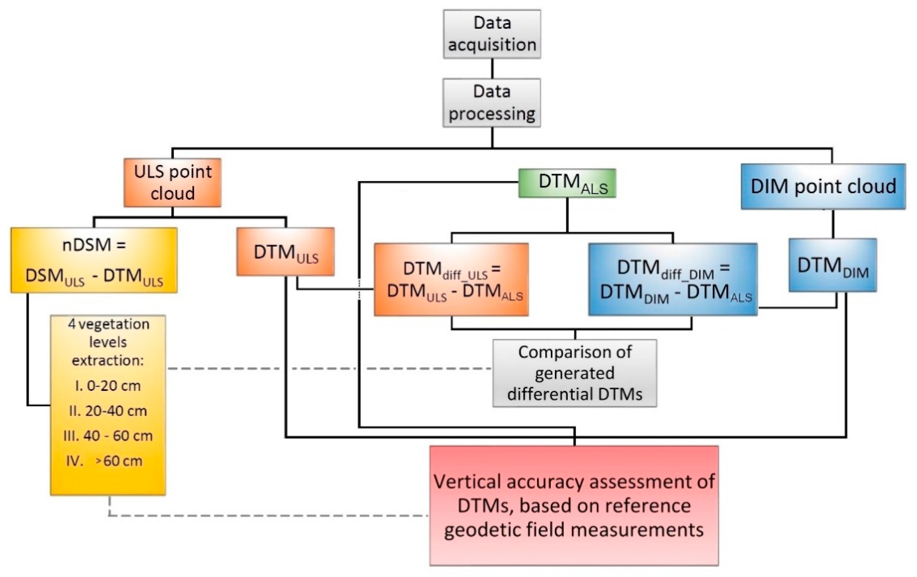
2.4. Methodology of Accuracy Assessment

The accuracy assessment of the ULS and DIM point clouds was conducted using a geodetic survey, and it referred to the archival ALS data. Within the accuracy examination, the influence of the vegetation on two basic techniques that deliver point cloud data was examined: Image-matching (DIM) and laser scanning from the UAV (ULS). The accuracy assessment methodology is presented in Figure 6.
It is difficult to compare whole point clouds with different characteristics and genesis. It was therefore decided to analyze the terrain models generated from two types of point clouds, because this product is the goal of most studies that use point cloud processing. Subsequently, the following elevation models were generated in the ArcMap software, providing listed parameters during their creation:
  • DTM from ULS data (DTMULS): for each cell of a 0.25 and 0.5 m grid, the height value was calculated by averaging observations (points); in the cases of cells without points inside, the Natural Neighbor interpolation method was used;
  • DSM from ULS data (DSMULS): for each cell of a 0.25 and 0.5 m grid, the height value was calculated by picking the maximum value from observations (points); in the cases of cells without points inside, the Natural Neighbor interpolation method was used;
  • DTM from DIM point cloud (DTMDIM): for each cell of a 0.25 and 0.5 m grid, the height value was calculated by averaging observations (points); in the cases of cells without points inside, the Natural Neighbor interpolation method was used.
DTMs with a 1-m resolution are usually used in hydrologic services, but in this article, DTMs with grid sizes of 0.25 and 0.5 m were generated, which appeared to be adequate for this type of application. Moreover, in a more detailed DTM (e.g., 0.1 m), more outliers can be noticed, which could be caused by small objects, such as stones or small holes. This finding might negatively influence the DTM during the interpretation. To define the influence of the interpolation and grid resolution, it was decided to analyze DTM in a 0.25 m resolution. A smaller grid size in this experiment was not well justified, due to the density of points in the ground class, which was less than 10 points per square meter for the ULS. The DIM point cloud density was much higher due to having a small GSD, and a resolution of 0.25 m was fine. When creating DTMs, only the “ground” classes from the ULS point cloud and the filtered DIM point cloud were used. The generation of DSMULS and DTMULS enabled the computation of the nDSM (normalized Digital Surface Model) in presenting the relative height of the land cover, which was a result of the difference between the DSMULS and DTMULS. The nDSM was used to determine the vegetation height levels every 20 cm in the test area. In this way, the study area was divided into four areas, which corresponded to the following vegetation height levels: I. 0–20 cm; II. 20–40 cm; III. 40–60 cm; and IV. over 60 cm. Such a division helped in the assessment of vegetation influence on accuracy depending on its height. Class I covered 2% of the test area, Class II—28%, Class III—38%, and Class IV—32%.
The next step was the evaluation of the elevation data, in comparison to the GNSS-RTK survey. Deviations between the raster values generated by the DTMs and the points measured in the field were analyzed. In the last step of the experiment, differential rasters, specifically DTMdiff_ULS and DTMdiff_DIM, were generated to compare the two tested techniques (high density UAV laser scanning and dense image matching) with ALS data that was used for levees inventory for years. These rasters represented elevation differences between the two models and were used in the accuracy assessment of the DTMs, based on a comparison to the ALS data. In this approach, the deviations of the rasters from the reference model, pixel by pixel, were investigated by providing the necessary statistics. Example visualizations of a fragment of generated DTMs, and the results of their subtraction, are presented in Figure 7.

3. Results

The vertical accuracy of the DTMs obtained from DIM and the ULS was analyzed first, in reference to the geodetic data. DTMs were compared with the GNSS terrain surveying. In the second part of the analysis, the differential DTMs were calculated, using the airborne laser scanning data to compare the tested techniques with the technique commonly applied. In both approaches, the analysis was conducted according to the earlier assumed areas of the four vegetation levels.

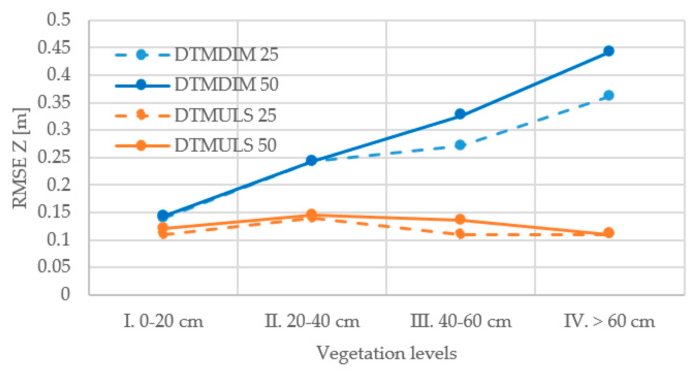
3.1. Accuracy Assessment of DTMs, Based on Surveying Field Measurements

In the first part of the vertical accuracy assessment, 193 checkpoints measured with GNSS-RTK technology were used. The RMSEZ was calculated, based on the differences between the Z coordinate of a check point and the corresponding DTM cell value, which is shown in Table 3.
The analysis using geodetic field measurements confirms a known statement, that the LiDAR techniques can measure the terrain covered with vegetation more accurately than the photogrammetric method. In case of DTMDIM, the increase in the RMSEZ with the vegetation height was clearly noticed, even if the number of points for the medium vegetation was lower. On the other hand, for the ULS data, the RMSEZ value was comparable for each vegetation height level and both tested DTM resolutions. However, these two techniques (ULS and DIM) gave comparable results in the case of vegetation with a height of 0–20 cm, which was useful information considering the very high resolution of the UAV-based images, and the high density of the ULS point clouds.
To illustrate the impact of the accuracy of both elevation data sets obtained from the UAV, an example cross-section is shown in Figure 8. It can be easily noticed that the DTMDIM profile was located above the DTMALS. The influence of the vegetation was also clearly seen here. The differences between the DTMs present the decimeter value, for the sloped part of the levee in this cross-section. This finding was comparable to the differences in the vegetation height of 20–40 cm. Additionally, in the levee crown, the profile of a road could be seen, where the vegetation was lower than 20 cm. The DTMDIM profile, corresponded here to the DTMs from LiDAR (both: ULS and ALS). According to the ULS, the DTMULS, and DTMALS profiles corresponded with each other along the whole length of the cross section, which indicated a visible ability of penetration through vegetation, for the laser scanner mounted on the UAV and the laser scanner on the airplane.

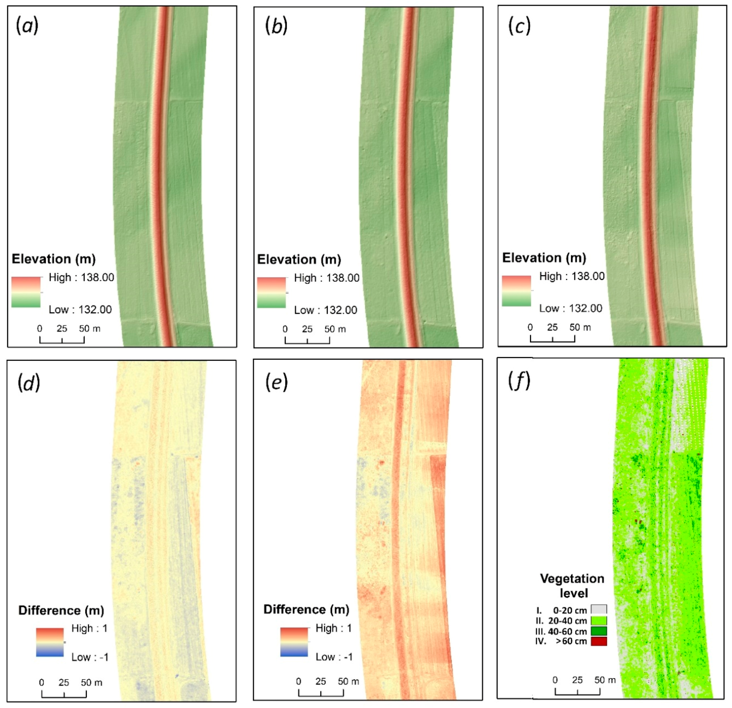
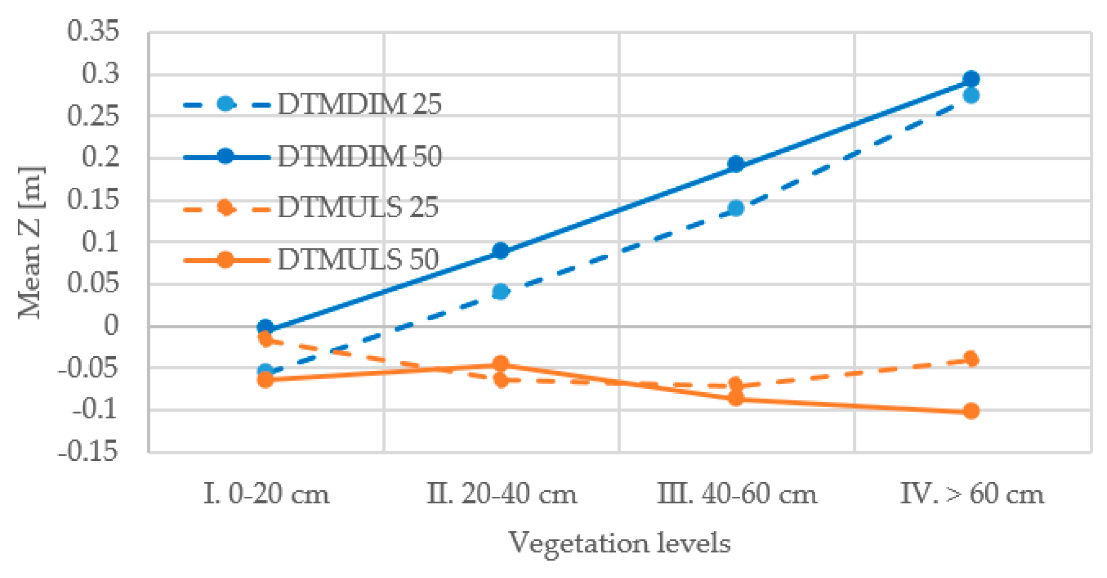
3.2. The Comparison of the DTMs with ALS Data

In the next step of the vertical accuracy assessment, statistical parameters, such as the Mean value and Standard deviation (STD), were calculated for each differential DTM raster in two spatial resolutions, with respect to the model from the airborne laser scanning data. The authors wanted to compare two extremely dense datasets, to the commonly used technique for DTM applications on levee monitoring. Statistics were provided with reference to four vegetation height levels.
In Table 4, the results of the accuracy assessment on the DTMs, based on the differential DTMs referred to DTMALS, are presented. It could be seen again that for the DIM, the influences of the vegetation on the accuracy of the DTM by increasing the mean value of the elevation difference was noticed (see the result for higher vegetation levels and both resolutions). For DTMDIM, the differences had positive values for low and medium vegetation (>20 cm), which proved the obvious lack of penetration through vegetation for the photogrammetric approach, and could suggest that the ULS data had a density of several dozen per square meter; which meant that more detailed data could be obtained by DIM than by ALS. In Figure 9 and Figure 10, the corresponding results from Table 3 and Table 4 are presented.

4. Discussion

To evaluate the DTMs, GNSS-RTK measurements were collected. A total of 193 measurements were made and divided into areas of four land cover classes. This approach allowed us to reliably determine the DTM accuracy of the models created with both technologies: Dense image matching and UAV laser scanning. In the experiment, a clearly visible gradual increase in the error of the terrain model created from the UAV photographs with higher vegetation was noticed. A decrease in the accuracy of 0.10 m, for every 20 cm of vegetation height, was observed in the experiment. This trend was observed for both DTM resolutions: 25 cm and 50 cm; however, slightly better accuracy could be observed for DTMDIM with a cell size of 25 cm. Such dependencies could not be observed in the case of models created from the ULS data.
Comparing the results between ULS and DIM, there was no significant difference in the vegetated areas which have a height of less than 20 cm, where the accuracy of both models and both resolutions compared to GNSS-RTK was between 0.11 and 0.14 cm. Therefore, when using DTM collected with the DIM algorithm, it is reasonable to limit the area of its analysis to areas with this type of coverage, such as in the tests presented in References [4,36].
For the assessment of data quality, a comparison to the airborne laser scanning data was also conducted and due to its accuracy, it cannot be a reference dataset, such as the GNSS-RTK measurements in the first part of the analysis. Overall, ALS provided the DTM models with higher accuracy than the image-matching technique, which is stated in Reference [3], where the DTMALS were compared with a few DTMs generated in two different software photogrammetric applications. Given the supremacy of the LiDAR data, the UAV measurements are often contrasted with ALS as a low-cost solution. In the experiment presented in this paper, a gradual increase in the Mean value of the DTM height difference between the UAV photogrammetric model and the ALS model was observed, and it increased together with the height of the vegetation. This relation could be easily explained by the passive nature of the optical sensor in the case of the images that cannot penetrate the vegetation, and thus, the impact of the vegetation on the created model could not be removed even with filtering algorithms. Of course, the problem of the influence of the vegetation on the results of the image matching was observed earlier in References [36,37], which resulted in the application of cloud point filtering methods to software (Pix4D Mapper, Agisoft Photoscan) or in research studies [18,19]. It must be also mentioned that higher overlap could minimize this problem. When undertaking a drone-based photogrammetric survey, the recommendation is to ensure overlaps of at least 70% and ideally more than 80%, even in corridor mapping [4,36,38] by using image-matching algorithms. In our research, overlap of 70/50% was defined. This caused the levee located in a middle of the flight corridor to be always presented in at least 6–8 photos; however these flight parameters allowed us to achieve satisfactory results. It can be assumed that slightly higher overlaps would not bring much better results. The test side was almost an uncovered area, and higher overlaps help in case of medium and high vegetation to generate proper DSM by avoiding occluded areas. In case of low vegetation, we proved that DIM could provide accurate DTMs for low vegetation, see the results in Table 2.
The analysis performed for the ULS data did not show any similar relationship. For all of the vegetation classes (every 20 cm of its height), the results were comparable to surveying measurements and ALS data. Considering the resolution of the DTM, the difference in the vertical accuracy was very small. It was caused by appropriate settings of DTMULS generation with respect to the data density [39]. However, having two datasets with extreme density (GSD and ULS point cloud density), the results proved that the resolution of DTM had more impact on the photogrammetric data. In the comparison to ALS data, it was also visible that regardless of the vegetation height, the ULS model was several centimeters (0.05 to 0.10 m) below the ALS model. This finding was confirmed by the Mean value of the height difference between the DTM and GNSS-RTK control points. For the ALS data, the Mean value with reference to geodetic measurements was 0.09 m, and for ULS, it was always in a range from 0.01 to 0.04 m (approximately 0.02 m), without influence of the resolution of the DTMs and vegetation height. This finding confirmed that the extreme density of LiDAR data was also crucial when very accurate DTM was required.
Referring to the issue related to point cloud filtering, both data sources, ULS and DIM, provided good results in the case of removal of large objects, such as trees [19]. The ratio of bare ground points with respect to all of the collected points was calculated. The ratio was equal to 95%, 5%, and 69% for DIM, ULS, and ALS, respectively. Using the algorithms in Agisoft, most of the points were classified as ground. Referring to the dense ULS point cloud, only a small percent of the points was found as ground points in contrast to ALS points, where 69% were classified as ground. Most of the ULS points were classified as low/medium vegetation, whilst the large group of ALS points must be in the “ground” class because the density of these data was a few points per square meter. ALS point clouds were classified automatically with manual correction (99% correctness of “ground class” and 95% for others), with hillshade model verification and evaluation based on numerous control points [35] before acceptance into the national repository. To assume the results of point cloud filtering, the difference was caused by the characters of the data as defined by its source: the technology and the platform. The influence of the uniform vegetation surfaces, such as grass or bushes, on the elevation models created with image matching could not be removed with point cloud filtering algorithms. This aspect was a crucial disadvantage of this technique.

5. Conclusions

Currently, a large increase in the density of point clouds can be observed, regardless of their generation by LiDAR or image-matching. The amount of such data makes it necessary to look at the derived DTM accuracy again, when this product can be generated from an extremely dense point cloud. The presented analysis of such datasets has usually indicated that ULS technology is more accurate than DIM, according to the vertical accuracy analysis in areas covered by vegetation. This conclusion is very important for data collected in seasons with developed vegetation. For both the DIM of very high-resolution images and the ULS, the source point cloud was filtered to obtain the points that represent the ground. In the experiment, four vegetation classes based on height values were distinguished. As a next step, the DTMDIM and DTMULS were evaluated based on the GNSS RTK measurement and compared with the airborne laser scanning. According to both analyses, the DTMULS presented better accuracy than DTMDIM on most vegetation classes. Moreover, the DTMULS accuracy was compared to the ALS results, and a higher penetration through the vegetation was observed for this technique, which was caused by a much higher density of the point cloud that could be offered by ULS from a multirotor platform. Referring to areas with very low vegetation (lower than 20 cm), the accuracy of both techniques was comparable. Additionally, it was clearly visible that there was approximately a 10-cm decrease in the accuracy of the DTM generated from the UAV images of extreme resolution, which were observed at every 20 cm of higher land cover. This trend was observed in both tested resolutions, and it can be slightly minimized with properly defined resolutions of the DTMs.
Although the UAV laser scanning technique has developed rapidly in recent years, the high prices of the sensors still render this technique expensive. Cameras which are mounted on the UAVs, are less expensive and more accessible than light laser scanners. However, the main disadvantage of the dense image matching is the lack of vegetation penetration. Therefore, in commercial programs, point cloud filtering is becoming a standard function. This technique is justified only in the case of bare ground terrain, e.g., open pit mines and areas covered with very low vegetation. The preferred season for this data collection is spring or late autumn. Referring to ULS data, it is possible to collect data in every season, but during summer, only this technique can be recommended, as LiDAR can generate more accurate DTMs than the photogrammetric technique, which considers UAV-based data.

Author Contributions

A.S., K.B., Z.K. conceived and designed the experiments; K.G. collected the datasets with the UAV platform, and A.S., W.O. and M.P performed the experiments; all of the co-authors wrote the paper.

Funding

The presented results are obtained within the realization of the project “Advanced technologies in the prevention of flood hazard (SAFEDAM)” financed by the National Centre for Research and Development in Defence, Security Programme; grant number DOB-BIO7/06/01/2015.

Acknowledgments

The authors would like to thank the MSP Marcin Szender and the Institute of Meteorology and Water Management—National Research Institute for their co-operation with the photogrammetric work, providing the UAV images and laser scanning data used in the present study.

Conflicts of Interest

The authors declare no conflict of interest.

References

  1. Baltsavias, E.P. A comparison between photogrammetry and laser scanning. ISPRS J. Photogramm. Remote Sens. 1999, 54, 83–94. [Google Scholar] [CrossRef]
  2. Gehrke, S.; Morin, K.; Downey, M.; Boehrer, N.; Fuchs, T. Semi-global matching: An alternative to LIDAR for DSM generation. In Proceedings of the 2010 Canadian Geomatics Conference and Symposium of Commission I, Calgary, AB, Canada, 14–18 June 2010; Volume 2, p. 6. [Google Scholar]
  3. Ressl, C.; Brockmann, H.; Mandlburger, G.; Pfeifer, N. Dense Image Matching vs. Airborne Laser Scanning–Comparison of two methods for deriving terrain models. Photogramm. Fernerkund. Géoinf. 2016, 2016, 57–73. [Google Scholar] [CrossRef]
  4. Tournadre, V.; Pierrot-Deseilligny, M.; Faure, P.H. UAV photogrammetry to monitor dykes-calibration and comparison to terrestrial Lidar. Int. Arch. Photogramm. Remote Sens. Spat. Inf. Sci. 2014, 40, 143–148. [Google Scholar] [CrossRef]
  5. Markiewicz, J.S.; Zawieska, D. Terrestrial scanning or digital images in inventory of monumental objects?—Case study. Int. Arch. Photogramm. Remote. Sens. Spat. Inf. Sci. 2014, 40, 395–400. [Google Scholar] [CrossRef]
  6. Nadal-Romero, E.; Revuelto, J.; Errea, P.; López-Moreno, J.I. The application of terrestrial laser scanner and SfM photogrammetry in measuring erosion and deposition processes in two opposite slopes in a humid badlands area (central Spanish Pyrenees). Soil 2015, 1, 561–573. [Google Scholar] [CrossRef] [Green Version]
  7. Riquelme, A.; Cano, M.; Tomás, R.; Abellán, A. Identification of Rock Slope Discontinuity Sets from Laser Scanner and Photogrammetric Point Clouds: A Comparative Analysis. Procedia Eng. 2017, 191, 835–845. [Google Scholar] [CrossRef]
  8. Bakuła, K.; Stępnik, M.; Kurczyński, Z. Influence of Elevation Data Source on 2D Hydraulic Modelling. Acta Geophys. 2016, 64, 1176–1192. [Google Scholar] [CrossRef]
  9. Lowe, D.G. Distinctive image features from scale-invariant keypoints. Int. J. Comput. Vis. 2004, 60, 1–110. [Google Scholar] [CrossRef]
  10. Hirschmuller, H. Stereo processing by semiglobal matching and mutual information. IEEE Trans. Pattern Anal. Mach. Intell. 2008, 30, 328–341. [Google Scholar] [CrossRef] [PubMed]
  11. Furukawa, Y.; Ponce, J. Accurate, dense, and robust multiview stereopsis. IEEE Trans. Pattern Anal. Mach. Intell. 2010, 32, 1362–1376. [Google Scholar] [CrossRef] [PubMed]
  12. Remondino, F.; Spera, M.G.; Nocerino, E.; Menna, F.; Nex, F. State of the art in high density image matching. Photogramm. Rec. 2014, 29, 144–166. [Google Scholar] [CrossRef]
  13. Jensen, J.L.; Mathews, A.J. Assessment of image-based point cloud products to generate a bare earth surface and estimate canopy heights in a woodland ecosystem. Remote Sens. 2016, 8, 50. [Google Scholar] [CrossRef]
  14. Fernández-Hernandez, J.; González-Aguilera, D.; Rodríguez-Gonzálvez, P.; Mancera-Taboada, J. Image-Based Modelling from Unmanned Aerial Vehicle (UAV) Photogrammetry: An Effective, Low-Cost Tool for Archaeological Applications. Archaeometry 2015, 57, 128–145. [Google Scholar] [CrossRef]
  15. Goncalves, J.A.; Henriques, R. UAV photogrammetry for topographic monitoring of coastal areas. ISPRS J. Photogramm. Remote Sens. 2015, 104, 101–111. [Google Scholar] [CrossRef]
  16. Hodgson, M.E.; Jensen, J.R.; Schmidt, L.; Schill, S.; Davis, B. An evaluation of LIDAR- and IFSAR-derived digital elevation models in leaf-on conditions with USGS Level 1 and Level 2 DEMs. Remote Sens. Environ. 2003, 84, 295–308. [Google Scholar] [CrossRef]
  17. Simpson, J.E.; Smith, T.E.; Wooster, M.J. Assessment of Errors Caused by Forest Vegetation Structure in Airborne LiDAR-Derived DTMs. Remote Sens. 2017, 9, 1101. [Google Scholar] [CrossRef]
  18. Serifoglu, C.; Gungor, O.; Yilmaz, V. Performance evaluation of different ground filtering algorithms for UAV-based point clouds. Int. Arch. Photogramm. Remote Sens. Spat. Inf. Sci. 2016, 41, 245–251. [Google Scholar] [CrossRef]
  19. Wallace, L.; Luckier, A.; Malenovský, Z.; Turner, D.; Vopěnka, P. Assessment of forest structure using two UAV techniques: A comparison of airborne laser scanning and structure from motion (SfM) point clouds. Forests 2016, 7, 62. [Google Scholar] [CrossRef]
  20. Gruszczyński, W.; Matwij, W.; Ćwiąkała, P. Comparison of low-altitude UAV photogrammetry with terrestrial laser scanning as data-source methods for terrain covered in low vegetation. ISPRS J. Photogramm. Remote Sens. 2017, 126, 168–179. [Google Scholar] [CrossRef]
  21. Harwin, S.; Lucieer, A. Assessing the accuracy of georeferenced point clouds produced via multi-view stereopsis from unmanned aerial vehicle (UAV) imagery. Remote Sens. 2012, 4, 1573–1599. [Google Scholar] [CrossRef]
  22. Tscharf, A.; Rumpler, M.; Fraundorfer, F.; Mayer, G.; Bischof, H. On the use of UAVs in mining and archaeology-geo-accurate 3D reconstructions using various platforms and terrestrial Views. ISPRS Ann. Photogramm. Remote Sens. Spat. Inf. Sci. 2015, 2, 15–22. [Google Scholar] [CrossRef]
  23. Fonstad, M.A.; Dietrich, J.T.; Courville, B.C.; Jensen, J.L.; Carbonneau, P.E. Topographic structure from motion: A new development in photogrammetric measurement. Earth Surf. Process. Landf. 2013, 38, 421–430. [Google Scholar] [CrossRef]
  24. Uysal, M.; Toprak, A.S.; Polata, N. DEM generation with UAV Photogrammetry and accuracy analysis in Sahitlerhill. Measurement 2015, 73, 539–543. [Google Scholar] [CrossRef]
  25. Mårtensson, S.G.; Reshetyuk, Y. Height uncertainty in digital terrain modelling with unmanned aircraft systems. Surv. Rev. 2017, 49, 312–318. [Google Scholar] [CrossRef]
  26. Petrie, G. Current developments in airborne laser scanners suitable for use on lightweight UAVs: Progress is being made! GeoInformatics 2013, 16, 16–22. [Google Scholar]
  27. Pilarska, M.; Ostrowski, W.; Bakuła, K.; Górski, K.; Kurczyński, Z. The potential of light laser scanners developed for unmanned aerial vehicles-the review and accuracy. Int. Arch. Photogramm. Remote Sens. Spat. Inf. Sci. 2016, 42, 87–95. [Google Scholar] [CrossRef]
  28. Amon, P.; Riegl, U.; Rieger, P.; Pfennigbauer, M. UAV-based laser scanning to meet special challenges in lidar surveying. Geomat. Indaba Proc. 2015, 2015, 138–147. [Google Scholar]
  29. Chaponnière, P.; Allouis, T. The YellowScan Surveyor: 5 cm Accuracy Demonstrated Study Site and Dataset. 2 October 2016. Available online: http://www.microgeo.it/public/userfiles/Droni/YellowScanSurveyor_whitePaper_accuracy.pdf (accessed on 31 March 2018).
  30. Bakuła, K.; Ostrowski, W.; Szender, M.; Plutecki, W.; Salach, A.; Górski, K. Possibilities for Using LIDAR and Photogrammetric Data Obtained with Unmanned Aerial Vehicle for Levee Monitoring. Int. Arch. Photogramm. Remote Sens. Spat. Inf. Sci. 2016, XLI-B1, 773–780. [Google Scholar] [CrossRef]
  31. Bakuła, K.; Salach, A.; Zelaya Wziątek, A.; Ostrowski, W.; Górski, K.; Kurczyński, Z. Evaluation of the accuracy of lidar data acquired using a UAS for levee monitoring: Preliminary results. Int. J. Remote Sens. 2017, 38, 2921–2937. [Google Scholar] [CrossRef]
  32. Pfeifer, N.; Mandlburger, G.; Otepka, J.; Karel, W. OPALS—A framework for Airborne Laser Scanning data analysis. Comput. Environ. Urban Syst. 2014, 45, 125–136. [Google Scholar] [CrossRef]
  33. Jozkow, G.; Wieczorek, P.; Karpina, M.; Walicka, A.; Borkowski, A. Performance Evaluation of sUAS Equipped with Velodyne HDL-32E LiDAR Sensor. Int. Arch. Photogramm. Remote Sens. Spat. Inf. Sci. 2017, 42, 171–177. [Google Scholar] [CrossRef]
  34. Axelsson, P. Processing of laser scanner data—Algorithms and applications. ISPRS J. Photogramm. Remote Sens. 1999, 54, 138–147. [Google Scholar] [CrossRef]
  35. Kurczynski, Z.; Bakula, K. The selection of aerial laser scanning parameters for countrywide digital elevation model creation. In Proceedings of the International Multidisciplinary Scientific GeoConference: SGEM: Surveying Geology & mining Ecology Management, Albena, Bulgaria, 16–22 June 2013; Volume 2, pp. 695–702. [Google Scholar] [CrossRef]
  36. Tournadre, V.; Pierrot-Deseilligny, M.; Faure, P.H. UAV linear photogrammetry. Int. Arch. Photogramm. Remote Sens. Spat. Inf. Sci. 2015, 40, 327–333. [Google Scholar] [CrossRef]
  37. Turner, D.; Lucieer, A.; de Jong, S.M. Time series analysis of landslide dynamics using an Unmanned Aerial Vehicle (UAV). Remote Sens. 2015, 7, 1736–1757. [Google Scholar] [CrossRef]
  38. Rehak, M.; Skaloud, J. Fixed-wing micro aerial vehicle for accurate corridor mapping. ISPRS Ann. Photogramm. Remote Sens. Spat. Inf. Sci. 2015, II-1/W1, 23–31. [Google Scholar] [CrossRef]
  39. McCullagh, M.J. Terrain and surface modelling systems: Theory and practice. Photogramm. Rec. 1988, 12, 747–779. [Google Scholar] [CrossRef]
Figure 1. Platform Hawk Moth with its equipment: YellowScan Surveyor laser scanner and RGB camera Sony Alpha a6000.
Ijgi 07 00342 g001
Figure 2. The location of the area of interest in Poland: Levee in Annopol, located on the Vistula River.
Ijgi 07 00342 g002
Figure 3. Visualization of the example flight trajectory, control and check points signalized with chess planes from one flight mission.
Ijgi 07 00342 g003
Figure 4. Isometric view of color-coded elevation of a point cloud for the Annopol test area: (a) ULS-based—YellowScan Surveyor, (b) photogrammetric-based from Agisoft Photoscan.
Ijgi 07 00342 g004
Figure 5. Visualization of the example GNSS-RTK cross-section points.
Ijgi 07 00342 g005
Figure 6. Accuracy assessment methodology.
Ijgi 07 00342 g006
Figure 7. Fragment of the test area: created terrain models: DTMALS (a), DTMULS (b), DTMDIM (c), and their results in the subtraction of DTMdiff_ULS (d), DTMdiff_DIM (e), and vegetation height (f).
Ijgi 07 00342 g007
Figure 8. Cross-section of levee with 3 classes of vegetation: levee slope—vegetation of 20–40 cm (II); levee crown—vegetation up to 40 cm (III and IV); and driveway—vegetation less than 20 cm (I).
Ijgi 07 00342 g008
Figure 9. Vertical accuracy assessment of DTMDIM and DTMULS based on reference geodetic field measurements.
Ijgi 07 00342 g009
Figure 10. Comparison of DTMDIM and DTMULS, to DTMALS.
Ijgi 07 00342 g010
Table 1. Hawk Moth platform specification.
NameHawk Moth
DeveloperMSP
Empty weight8.5 kg
Max. payload4 kg
Average cruise speed5 m/s
Max. cruise speed12.5 m/s
Hovering time15 min (with 3 kg payload)
Sensor equipment1. ultralight laser scanner YellowScan Surveyor (Weight: 1.60 kg), Size (mm): 100 × 150 × 140)
2. RGB camera Sony Alpha a6000 (weight: 0.47 kg)(24.3 MPix APS-C CMOS sensor)
Table 2. Aerotriangulation results for 8 flight missions.
Number of Flight MissionNumber of PhotosControl PointsCheck Points
Number of Control PointsRMSX (m)RMSY (m)RMSZ (m)Number of Check PointsRMSX (m)RMSY (m)RMSZ (m)
1172110.0760.1210.10640.0840.1100.122
2173100.0550.0310.07750.0750.0280.082
3153100.0780.0420.01650.0670.0600.067
414980.0300.0320.02750.0280.0370.072
516880.0340.0310.05440.0520.0480.083
6176110.0490.0580.07240.0250.0550.076
715780.1180.0420.02640.0880.0540.064
813770.0470.0310.09340.0270.0820.101
Table 3. Vertical accuracy assessment of digital terrain models (DTMs), based on the reference geodetic field measurements (GNSS-RTK check points).
Vegetation Height levelsNumber of Check PointsDTMDIM 25DTMDIM 50DTMULS 25DTMULS 50DTMALS 50
Mean (m)RMSEZ (m)Mean (m)RMSEZ (m)Mean (m)RMSEZ (m)Mean (m)RMSEZ (m)Mean (m)RMSEZ (m)
I. 0–20 cm600.0620.1390.0640.1440.0050.1090.0050.1210.0910.115
II. 20–40 cm910.1810.2420.1770.2420.0370.1390.0350.145
III. 40–60 cm310.2050.2710.2480.3260.0080.1090.0090.135
IV. >60 cm110.2250.3610.4020.4420.0130.1100.0230.110
Table 4. Vertical accuracy assessment of DTMs, based on differential DTM referred to airborne laser scanning (ALS) data.
Vegetation Height LevelsArea (ha)DTM DIM 25DTM DIM 50DTM ULS 25DTM ULS 50
Mean (m)STD σ (m)Mean (m)STD σ (m)Mean (m)STD σ (m)Mean (m)STD σ (m)
I. 0–20 cm0.933−0.0560.305−0.0050.279−0.0180.145−0.0650.220
II. 20–40 cm13.9000.0390.2300.0880.338−0.0650.121−0.0470.299
III. 40–60 cm18.6160.1380.2420.1900.274−0.0710.160−0.0880.163
IV. >60 cm16.0670.2740.4070.2920.378−0.0410.291−0.1040.277

