Article

The Value of OpenStreetMap Historical Contributions as a Source of Sampling Data for Multi-Temporal Land Use/Cover Maps

Centre for Geographical Studies, Institute of Geography and Spatial Planning, Universidade de Lisboa, Rua Branca Edmée Marques, 1600-276 Lisboa, Portugal
*
Author to whom correspondence should be addressed.
ISPRS Int. J. Geo-Inf. 2019, 8(3), 116; https://0-doi-org.brum.beds.ac.uk/10.3390/ijgi8030116
Submission received: 30 November 2018 / Revised: 18 February 2019 / Accepted: 23 February 2019 / Published: 28 February 2019

Abstract

:
OpenStreetMap (OSM) is a free, open-access Volunteered geographic information (VGI) platform that has been widely used over the last decade as a source for Land Use Land Cover (LULC) mapping and visualization. However, it is known that the spatial coverage and accuracy of OSM data are not evenly distributed across all regions, with urban areas being likelier to have promising contributions (in both quantity and quality) than rural areas. The present study used OSM data history to generate LULC datasets with one-year timeframes as a way to support regional and rural multi-temporal LULC mapping. We evaluated the degree to which the different OSM datasets agreed with two existing reference datasets (CORINE Land Cover and the official Portuguese Land Cover Map). We also evaluated whether our OSM dataset was of sufficiently high quality (in terms of both completeness accuracy and thematic accuracy) to be used as a sampling data source for multi-temporal LULC maps. In addition, we used the near boundary tag accuracy criterion to assesses the fitness of the OSM data for producing training samples, with promising results. For each annual dataset, the completeness ratio of the coverage area for the selected study area was low. Nevertheless, we found high thematic accuracy values (ranged from 77.3% to 91.9%). Additionally, the training samples thematic accuracy improved as they moved away from the features’ boundaries. Features with larger areas (>10 ha), e.g., Agriculture and Forest, had a steadily positive correlation between training samples accuracy and distance to feature boundaries.

1. Introduction

Since the end of the 20th century, land use and land cover (LULC) maps have been extensively generated at different spatial and temporal scales. The 2000 Global Land Cover map [1] and the 2000 CORINE Land Cover (CLC) [2] map are two examples. Multi-temporal LULC maps can be used to monitor land changes over time, enabling the creation of indicators that can measure changes and support land management. Mapping results have a significant impact on our understandings of LULC patterns and can affect monitoring, characterization, and quantification outcomes. Nevertheless, one of the main challenges regarding LULC map production is the difficulty of distinguishing and accurately mapping land attributes.
Over the last decade, volunteered geographic information (VGI) platforms [3], as well as other data contributed by social network communities [4,5], have been widely used as sources for LULC mapping and visualizations [6,7,8,9,10,11,12,13]. Crowdsourced content from online platforms, accessed, and exchanged by citizens, has emerged as a supplementary data source with significant implications for LULC database production [14]. This nontraditional data source is not necessarily a substitute for official data, but is considered to be complementary [15].
OpenStreetMap (OSM) is a free, open-access VGI platform to which volunteers from all over the world collaboratively contribute data, and it is a particularly promising source of information for LULC analysis [10,16,17]. Several factors have been essential to its success, including its availability of up-to-date data with global coverage, improvements in data quality (mainly driven by an increase in the number of contributors over time) [11,18], and its extensive volume and variety of thematic attribute data [11]. OSM therefore has the potential for use in the long-term mapping and monitoring of LULC changes [6] and could plausibly be used to improve the production, verification, and validation of LULC maps [6,7,8,11,19,20,21]. A multi-temporal trajectory can be achieved using OSM data [22], not only for LULC mapping but also for ground-validated data creation [19].
However, it is known that both the spatial coverage and the accuracy of OSM data are not homogeneous across all regions [16,23], with urban areas being likelier to have promising contributions (in both quantity and quality) than rural areas [24,25]. Several authors have recently highlighted quality issues on VGI platforms [4,26,27,28,29,30,31,32]. OSM data still lack formal standards, such as those established by the International Organization for Standardization (ISO) 19157: 2013 Geographic information-Data quality [11,33]. Five data quality criteria are commonly mentioned in the literature: (1) Completeness, (2) temporal accuracy, (3) logical consistency, (4) positional accuracy, and (5) thematic accuracy [34,35,36].
The thematic accuracy [37] of the OSM platform’s LULC mapping is currently a hot research topic [7,9,10,11,34], and a number of studies have compared OSM data with authoritative reference data [6,7,16,33,35,38]. For example, two studies of mainland Portugal [6,7] found a total of 76.7% agreement between the data from OSM and CLC maps, with artificial surfaces, forests, and water bodies presenting promising results. Similarly, a study of Vienna [21] compared OSM data to data from the Global Monitoring for Environment and Security Urban Atlas (GMESUA) and found an agreement rate of 76% to 91%. More recently, another comparison of OSM and GMESUA data [8] found an agreement rate of about 90%.
Completeness accuracy [23] is also commonly used to assess OSM data since it allows for the evaluation of territorial coverage. It has been used mainly to evaluate the completeness of OSM’s data on road networks [22,39,40], buildings [23,41,42], and LULC features [6,9,34].

Related Works

Recent studies [43,44,45] have also included OSM contributors’ update history in data quality assessments. OSM full history file stores extra information associated with data contributions, such as timestamps that provide the exact date and time of contributions [39,40,41,46]. For example, one study [40] that assessed OSM’s road network completeness and positional accuracy using OSM data history concluded that the use of historical information improved the quality of OSM data by up to 14%. OSM data history can moreover be used for a number of different purposes [40] and allow for new perspectives on the reliability of OSM data at different scales and timeframes [22,40]. OSM data history is available since 2005.
In the present study, OSM data history has been accessed to generate different LULC datasets based on the contribution year (using the timestamps) in order to create regional and rural multi-temporal LULC maps. This had two primary purposes. First, we sought to evaluate the degree to which OSM datasets bounded by one-year timeframes agreed with extant authoritative datasets (i.e., CLC and the official Portuguese Land Cover Map—COS), using both completeness and thematic accuracy as quality parameters. Second, we sought to evaluate whether the OSM datasets were of sufficient quality to be used as sampling data sources for multi-temporal LULC maps. For this second assessment, we used near boundary tag accuracy (NBTA) to evaluate the fitness of the OSM data for producing training samples, by looking at the extent to which a feature’s proximity to a boundary influenced its attribute (tag) accuracy.
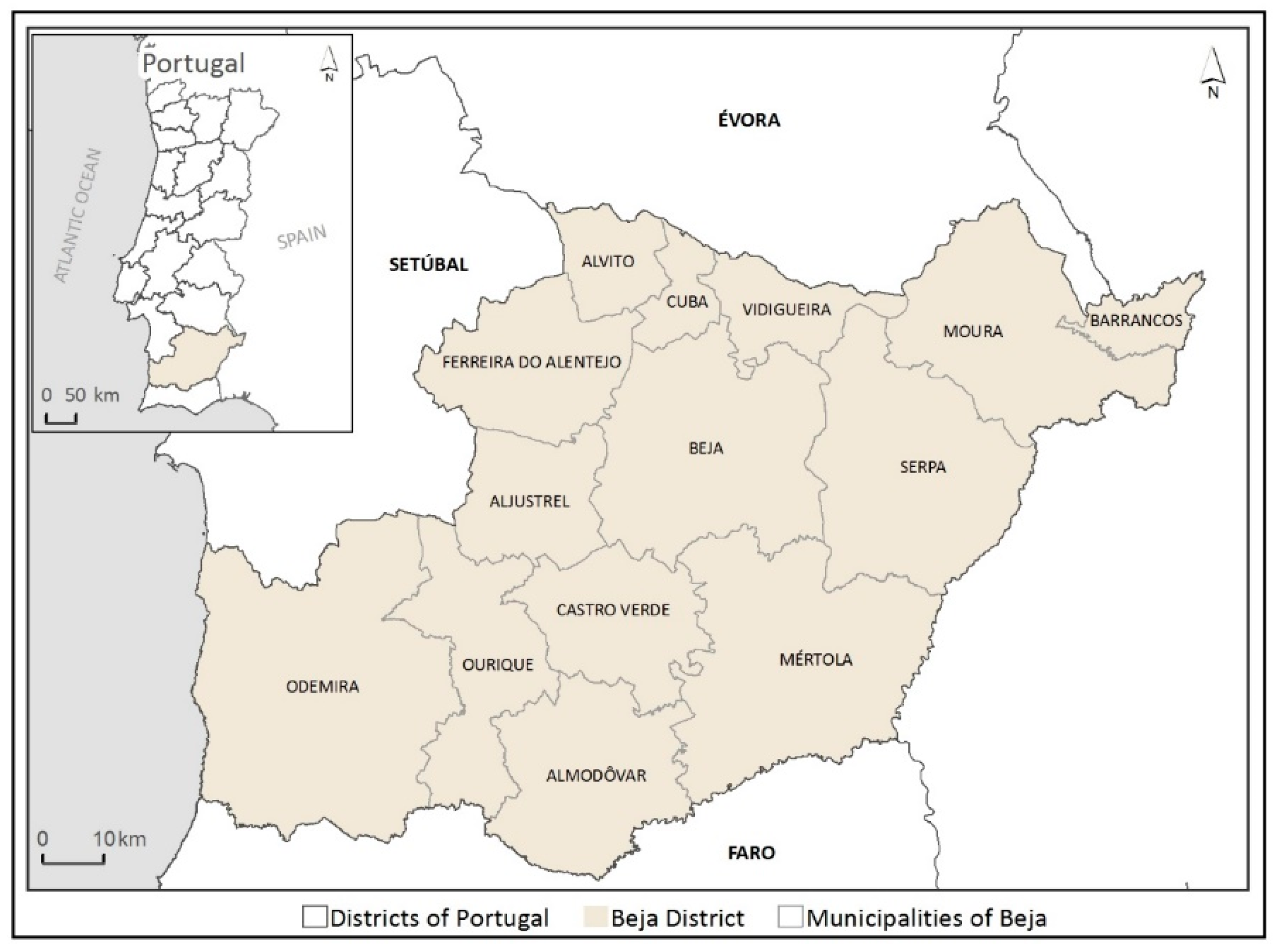
This research was conducted in the largest Portuguese district, Beja. It is a predominantly rural region with high natural and economic value, and is characterized by a mixed agro-silvo-pastoral ecosystem [47]. In addition, the region has recently undergone rapid LULC changes [47,48,49], and the limited number of references LULC data for this region emphasizes the importance of finding supplementary LULC data to support the identification and monitoring of these changes.
Our research is discussed in the rest of this paper. Section 2 describes the study area and our data. Section 3 details our methodology. Section 4 presents our OSM quality results. Finally, in Section 5 we discuss the implications and main conclusions of our results.

2. Study Area and Data

2.1. Study Area

Beja is a district located in the southeast of Portugal, in the Alentejo region (Figure 1). It is the largest Portuguese district, with an area of 10,229.05 km2, and as of 2011 it had a population of 152,758 residents [50]. Urban density is low, and agricultural and forest areas dominate. The southeastern part of the district is flat, while in the northern and western parts the extensive plains are intersected by tiny hills. The valley of the River Guadiana, which traverses the eastern part of the district in a north-south direction, is the district’s main geographical feature.

2.2. Datasets

2.2.1. The OSM Dataset and History File

OSM data can be freely downloaded, for example from Geofabrik or Planet OSM, in the form of raw datasets covering different regions (countries, continents, or any other administrative level) around the globe. OSM data represent physical features (objects) on the ground, and their tags (i.e., labels) are used to describe the objects (i.e., class description). The OSM data include a variety of physical feature types, with land use, natural features, waterways, amenities, and highways being the most commonly represented [51]. Feature descriptions can be found on the OSM wiki page (https://wiki.openstreetmap.org/wiki/Map_Features).
OSM history file includes records of all historical contributions, including recent ones, and are accessible as either XML or PBF formatted files. They provide a history of every modification made to a geographical feature’s shape or tag. This means that if, for example, a feature’s shape has been changed once, there will then be two entries for the same feature—the original feature and the modified one. A sample illustration and more information can be found in Nasiri et al. [40]. In the present study, we accessed the history file to see the timestamps (day/month/year and time) of each feature’s creation and modifications.

2.2.2. Official Reference Datasets

The two reference LULC datasets used in this study were the 2012 CLC and the 2015 official Portuguese COS. The CLC is produced by the Portuguese General Directorate for Territorial Development (DGT) in coordination with the European Environment Agency, while the COS is produced exclusively by the DGT. Both datasets are freely available for download from the DGT website (http://mapas.dgterritorio.pt/geoportal/catalogo.html), and both use hierarchical and a priori nomenclature systems. The COS nomenclature was produced to match the CLC one. Thus, despite the fact that COS has five disaggregation levels compared to the CLC’s three, the COS’s first three levels are similar to the three CLC levels, thereby enabling comparisons between them. The dataset characteristics and metadata are shown in Table 1, and their descriptive statistics are shown in Table 2. More details about their nomenclature characteristics can be seen in Estima and Painho [7].

3. Methods

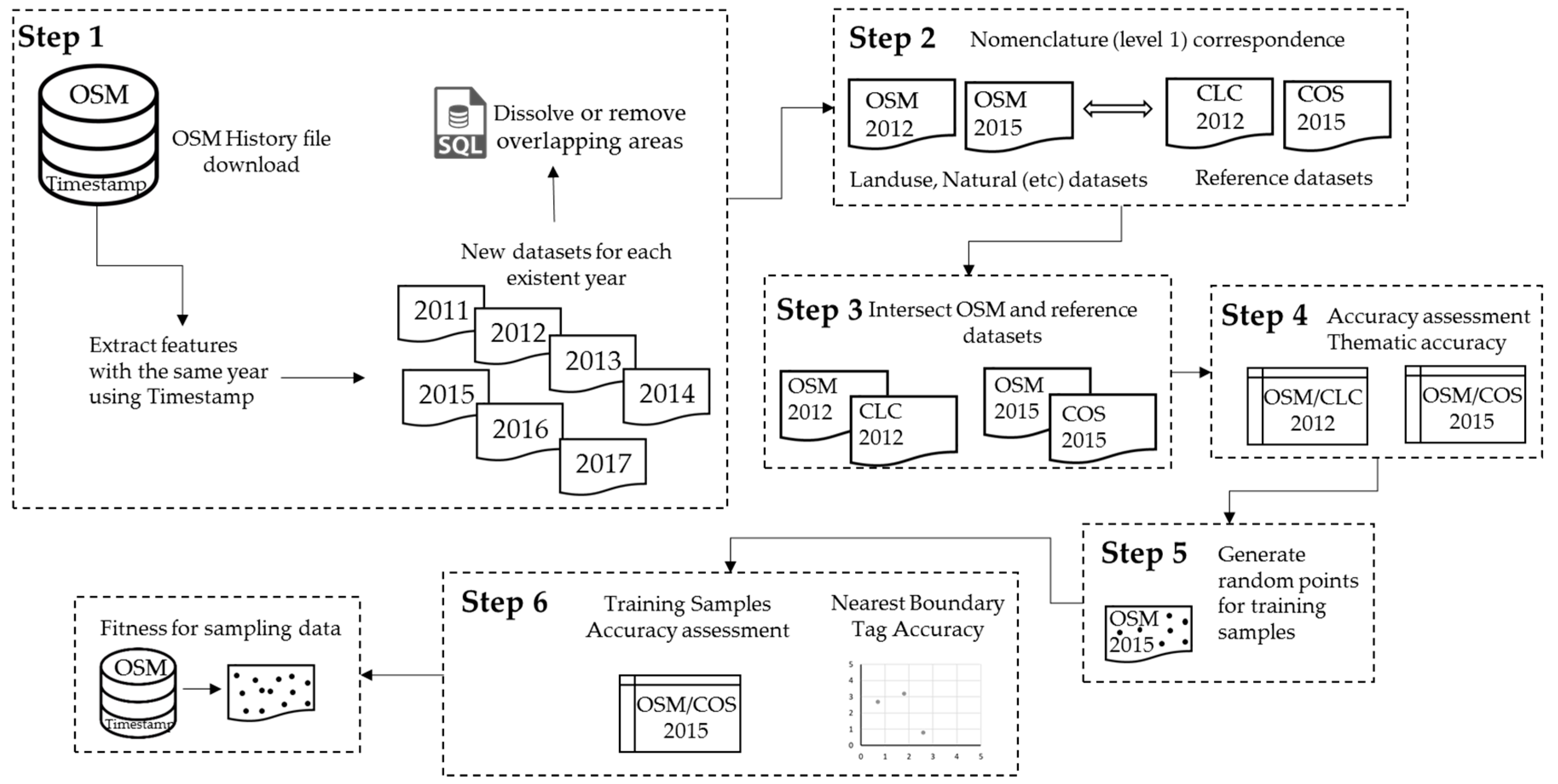
Figure 2 shows our main steps. Briefly, our first step was to download the OSM data history file and filter the contributions according to their timestamps. We obtained datasets for seven different years and resolved all logical inconsistencies, such as overlapping features. Second, we established a relationship between the OSM and CLC/COS first level of nomenclature. Third, we intersected the datasets to determine the area corresponding to the OSM dataset that matched the reference dataset. Fourth, we calculated the datasets’ completeness and thematic accuracies for 2012 and 2015. Fifth, random points were generated as training samples. Finally, in step six we calculated the NBTA for 2015.

3.1. Processing the OSM Datasets

We began by downloading from Geofabrik the latest OSM history file available at the time (7 May 2018) that covered Portugal. All OSM objects with the feature types of land use, natural features, airways, amenities, buildings, highways, historic features, leisure features, man-made features, power structures, public transportation, railroads, shops, sports, tourism, forests, and waterways were retrieved. We limited our results to features (polygons) found in the Beja district. By filtering the features by contribution year (using the timestamp data), we generated multi-temporal datasets that included only the features which were created or modified during any given year. We found contributions for seven different years (2011–2017). Since reference data for the study area only exists for 2012 (CLC) and 2015 (COS), we identified and selected all the OSM data contributions that had been created/modified in these two years (2012 and 2015) and used these two OSM datasets in our study for comparison with the reference datasets.
A common problem when processing OSM data is the presence of logical inconsistencies, such as overlapping features [6,9,34,35]. This problem is even more common when history files are used, since they contain records of every single modification. It is therefore essential to dissolve or remove the overlapping features in order to not overestimate areas and to ensure that only one attribute (tag) is kept for analysis [6,9,35]. To ensure logical consistency between the annual datasets, when overlapped features had the same attribute we dissolved the overlapping areas, while when the overlapped features’ attributes did not match the conflict areas were removed.
In addition, we examined the provenance of OSM data for our study area to confirm that there were no bulk imports from known sources (e.g., CLC; COS). In this study the polygons´ geometry for each reference dataset and both OSM datasets was compared by using the Feature Compare tool of ArcGIS 10.5 software.

3.2. Relationship between Dataset Nomenclatures

Several studies have stressed the difficulties of using datasets from different agencies due to the lack of direct relationships between their classes [6,9,35,52]. In Estima and Painho [6], the authors attempted to reconcile the three nomenclature levels of the CLC, the OSM land use feature, and the OSM natural areas feature, based on the official descriptions of the CLC and OSM classes. Given their remarkable results, we decided to partially follow their nomenclature correspondence for the first level of the CLC and COS nomenclature, namely, (1) artificial surfaces, (2) agricultural areas, (3) forests, (4) wetlands, and (5) water (see Table 3). For the purposes of the study, the OSM features type airways, amenities, buildings, highways, historic features, leisure features, man-made features, power structures, public transportation, railroads, shops, sports, and tourism were considered to be (1) artificial surfaces. The OSM feature type wood was classed as (3) forest, while the OSM feature type waterway was classed as (5) water.

3.3. Accuracy Assessment Criteria

3.3.1. OSM Completeness Accuracy

It can be difficult to draw definitive conclusions from OSM data due to the heterogeneity of contributions across different regions [23]. This challenge poses particular limitations when analyzing rural areas [16,53]. Accordingly, the completeness accuracy criterion is commonly used to assess the quality of OSM data [22,34,35]. Completeness accuracy is defined as the completeness of a dataset and measures the presence or absence of features. Typically, the total number of features is computed for point features, while for line features the total length is computed. These calculations are then compared to the reference dataset [23]. However, for polygon features, it is assumed that the overall area of the study area is the maximum area possible, and it is therefore not necessary to compare it to reference data [35].
In this study, completeness accuracy was calculated as a ratio of the OSM features’ overall area (AOSM) and the total area of the study area (ARef). It is presented here as a percentage, as described in Equation 1. A ratio of 100 means that the OSM dataset provides full coverage of the study area. This criterion was measured for all OSM dataset features for 2012 and 2015 for each LULC class.
Completeness = A OSM A Ref × 100

3.3.2. OSM Thematic Accuracy

Thematic accuracy is another common criterion used to evaluate the quality of OSM dataset features in LULC mapping [6,7,8,21]. Thematic accuracy describes the accuracy of the features’ attributes (tags) by computing the differences between OSM dataset features and those of the chosen reference datasets [35].
In this study, we used an overlap function to determine which features overlapped between the OSM datasets (2012 and 2015) and the reference datasets (CLC and COS, respectively). Following common statistical approaches [35,54], for each annual dataset the overlapping areas were computed in a confusion matrix, which presented the correct and incorrect mapped areas for each LULC class. The rows denote the occurrences of an actual class (OSM) and the columns denote the occurrences of reference data classes (CLC or COS). Several measures were obtained from this, including overall thematic accuracy, individual user accuracy, producer accuracy, and the Kappa index of agreement [34,35,55]. The overall thematic accuracy measure provides the overall percentage of the correctly mapped OSM features by dividing the correct mapped area by the total mapped area. User accuracy measures the probability that any given LULC class from an OSM dataset will actually match the reference dataset, while producer accuracy indicates the probability that a particular LULC class from the reference dataset is classified as such in OSM [35]. The Kappa index measures the degree of agreement between the OSM dataset and the reference dataset [55].

3.3.3. Near Boundary Tag Accuracy (NBTA)

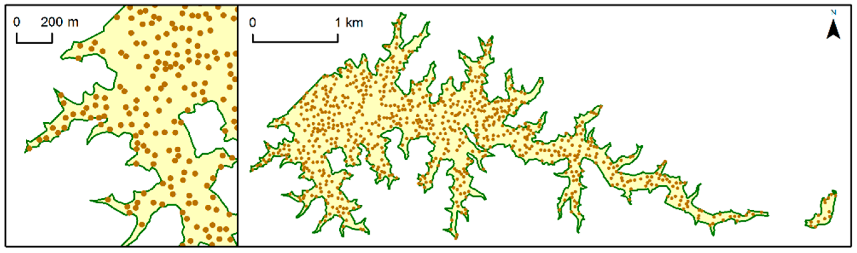
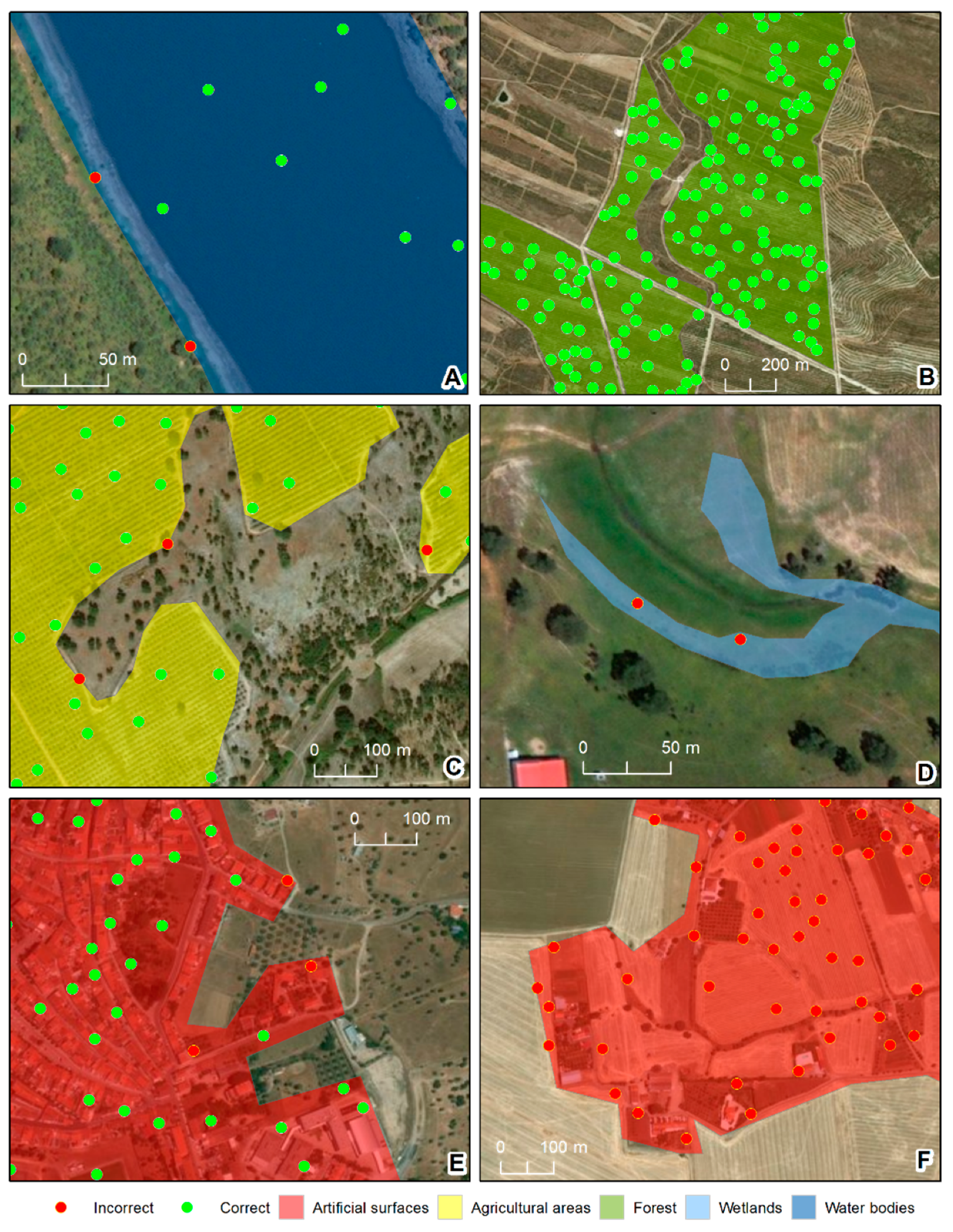
We also used NBTA to measure the fitness of the OSM data as a source of sampling data to support regional and rural LULC mapping. NBTA measures the extent to which the proximity of an OSM feature’s boundary influences the accuracy of the attribute (tag) in the training sample. We computed the NBTA for the most recent OSM dataset (2015). First, it was necessary to create training samples by generating random points inside the OSM features. Since OSM feature areas are very heterogeneous, it would be inappropriate specify an exact number of random points to be generated inside each OSM feature; instead, the total number of random points generated was proportional to the area of each OSM feature. In addition, the shortest distance allowed between any two randomly placed points was 30 m, because this is the most common spatial resolution of satellite images, such as Landsat (Figure 3). We used point features instead of polygon features since this minimized the effects of comparing data with different mapping scales. Each random point generated took the attribute of the corresponding OSM polygon feature.
Second, thematic accuracy was assessed following the same procedure described in 
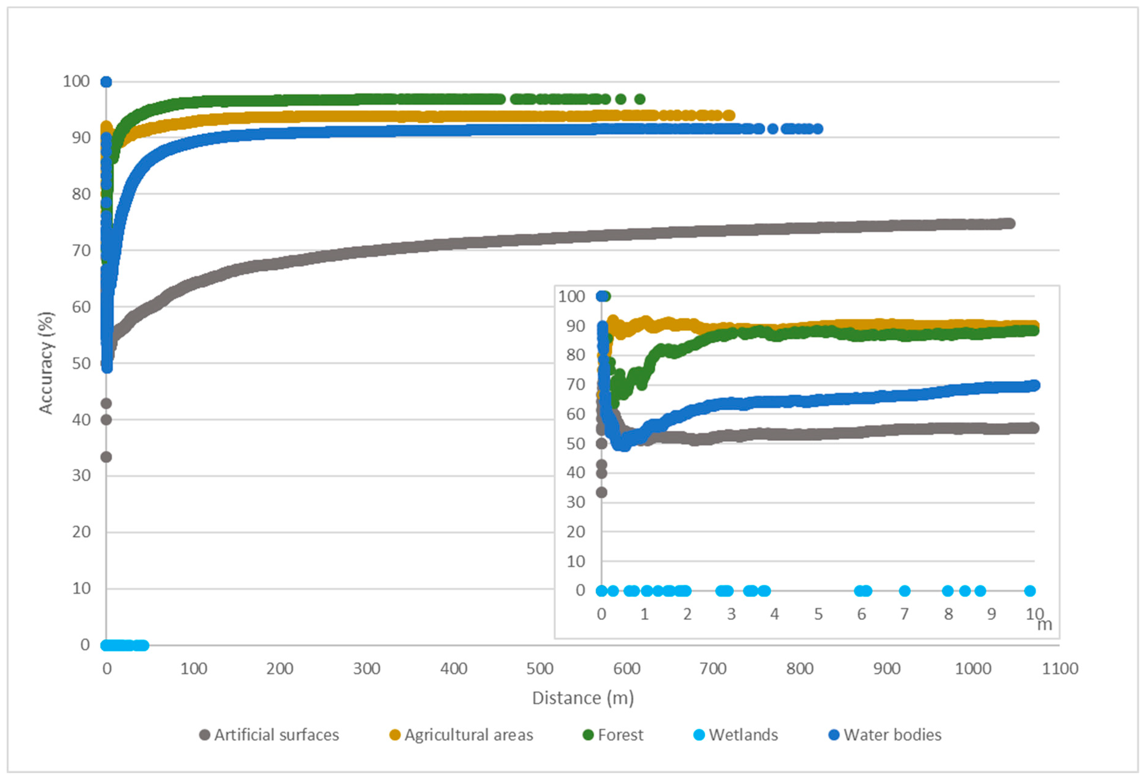
Section 3.3.2. Also, the Euclidean distance from each random point to the nearest segment of the OSM feature’s boundary was computed. The distance values (in ascending order) and the accumulated thematic accuracy were then plotted. The purpose of this process was to ascertain whether the training samples generated for each LULC class near the border of an OSM feature might be inherently less accurate.
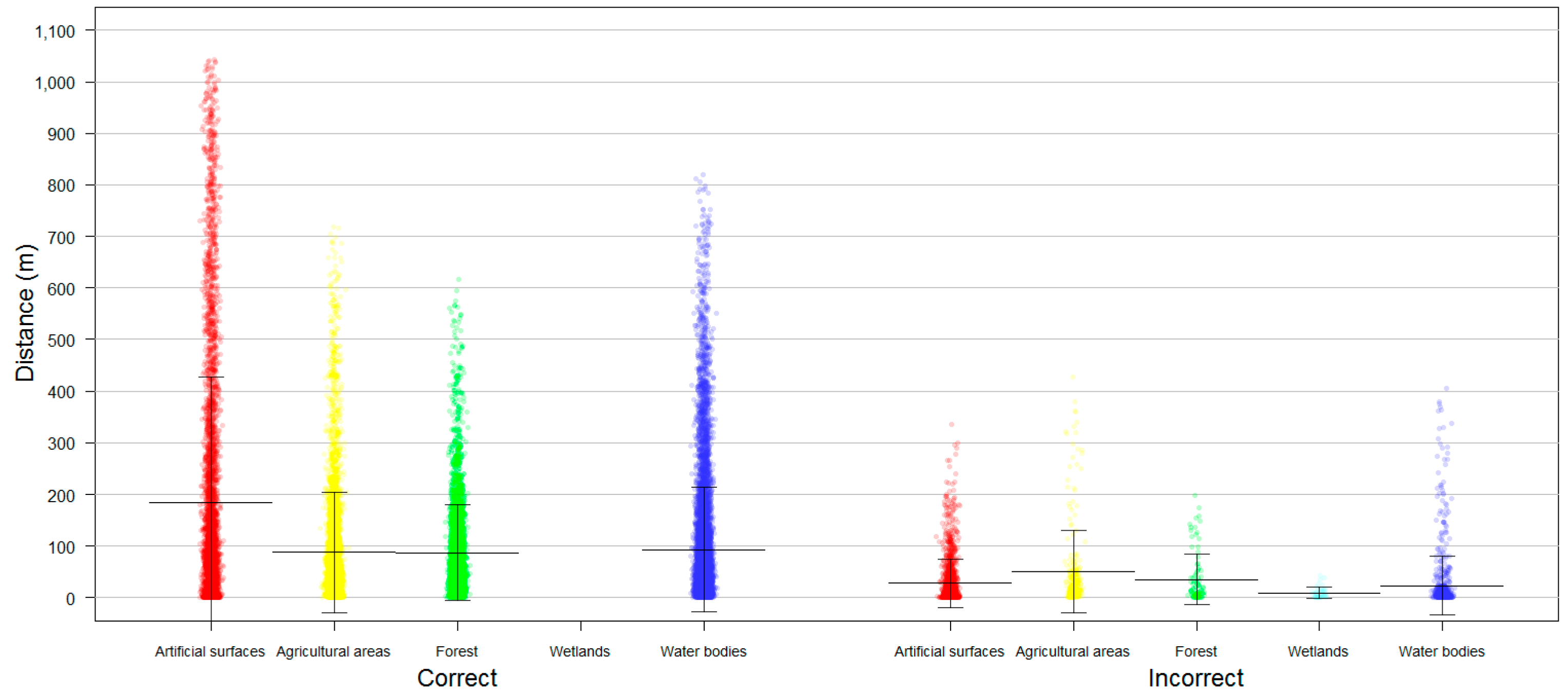
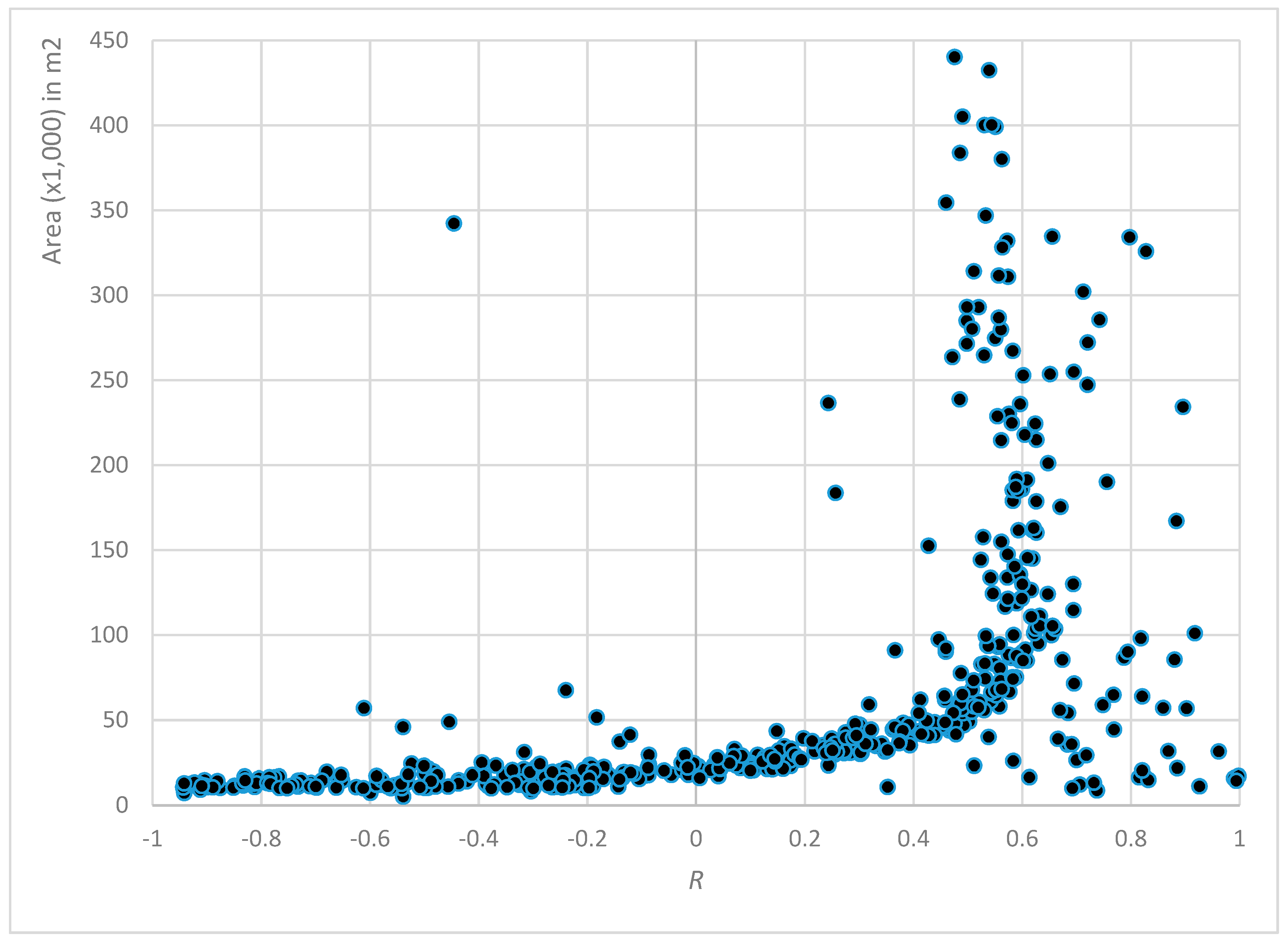
However, the relationship between the training samples accuracy and their proximity to the corresponding feature boundaries did not consider the influence of each feature area in explaining the degree of accuracy, since the distance to a feature boundary varies across feature areas. Are features with larger or smaller areas likely to have more or less accuracy? Therefore, the distance values from all training samples were standardized using the maximum and minimum distance values of the corresponding OSM feature. Similarly, the accumulated accuracy of all training samples was computed by considering each OSM feature. The relationship between a feature’s boundary proximity and its thematic accuracy is denoted by the Pearson correlation coefficient (R), which was calculated separately for each OSM feature. OSM features with fewer than three training samples were excluded from the analysis (20% of all polygons, for 2015), because when n = 2 the R coefficient would always be −1 or +1, except in the improbable circumstance that both y-values perfectly matched.

4. Results

4.1. OSM Dataset Analysis

The identification and selection of OSM data contributed in 2012 and 2015 allowed us to create two different datasets for analysis. However, these datasets presented some logical inconsistencies that had to be resolved. There were 994 and 2100 non-overlapping features in 2012 and 2015, respectively. After dissolving or removing the overlapping features following the procedure described in Section 3.1., the final datasets were comprised of 1215 and 2863 distinct features in 2012 and 2015, respectively.
The descriptive statistics for both years are presented in Table 4. It is notable that the total area covered increased significantly between 2012 and 2015 (+155%). In addition, between 2012 and 2015 the features’ minimum area doubled, while their maximum area increased by 2.5 times. As expected, the standard deviation measure also confirmed high variations between the features’ areas for each annual dataset, as most the natural/anthropological features fit power law (like) distributions.
In addition, the statistical analysis shows that the 98% of the features in 2012 OSM dataset and the 97% of the features in 2015 OSM dataset have less than 25 ha and the 76.13% of the features in 2012 OSM dataset, as well as the 79.9% of the features in 2015 OSM dataset have less than 1 ha. In this way we are able to verify that the OSM used data are not imported from the reference datasets since the CLC minimum area unit is 25 ha and COS minimum area unit is 1 ha. When we compared the geometry of the 2012 and 2015 OSM features with the CLC and COS datasets, less than 0.1% matching was obtained, proving that no bulk imports were made from these reference data.

4.2. OSM Completeness Accuracy

The completeness ratio of the coverage area for the selected study area has been increasing year after year (Table 5). However, in 2012, contributions covered less than 1% of the total district area, while in 2015 contributions covered about 1%. Following Table 6, Water was the largest LULC class in both annual OSM datasets (45% in 2012 and 46% in 2015). In 2012, agricultural areas represented about 40% of the total dataset, followed by artificial surfaces (16%), while in 2015 both classes were around 20%. In contrast, in 2012 forests were not significantly represented, but in 2015 they accounted for 14% of the total dataset. It is also interesting to note that in 2012 there were only four LULC classes represented (artificial surfaces, agricultural areas, forests, and water), while in 2015 there were five, due to the additional presence of wetlands. However, wetlands accounted for less than 0.001% of total coverage. In addition, the relationship between the total features’ contributions and the corresponding area for each class demonstrated that both agricultural areas and water areas had consistently huge polygons drawn by contributors.

4.3. OSM Thematic Accuracy

A confusion matrix was computed for each annual dataset (Table 7 and Table 8) in order to evaluate its thematic accuracy. The results showed that thematic accuracy was 77.3% in 2012 and 91.9% in 2015, indicating a very high agreement (i.e., accuracy) between the 2015 OSM dataset and the reference dataset (COS). However, there was a wide variation among the accuracy values for each class. In particular, agricultural areas were highly accurate, with a 99.8% user accuracy rate in 2012 and a 94.5% user accuracy rate in 2015, suggesting that the areas classified by contributors as agricultural areas closely matched those in the reference datasets (CLC and COS, respectively). While the producer’s accuracy rates were not quite as high (71.9% in 2012 and 79.1% in 2015), they were still high enough to suggest that this class was correctly shown on the OSM. Artificial surfaces also had consistently high accuracy values; in 2012, the user and producer accuracy rates were 70.9% and 75.5%, respectively, and in 2015 they increased to 80.9% and 95.3%, respectively.
Other classes showed a strong increase in user accuracy between 2012 and 2015. User accuracy for forests jumped from 0% in 2012 to more than 97% in 2015, and user accuracy for water increased from about 60% in 2012 to over 94% in 2015. In contrast, producer accuracy for water was very high in both years (about 99.7%). Producer accuracy for forests improved from 0% in 2012 to over 88% in 2015. However, wetlands had null values for both user and producer accuracy in both years (0%). Overall, following the standards set by [55], the Kappa index indicated substantial agreement between the OSM and reference maps in 2012 (0.65) and an almost perfect agreement in 2015 (0.88).

4.4. Assessing the Fitness of OSM Data

Using the method described in Section 3.3.3., about 24,175 random points were generated from the 2015 OSM dataset features. We evaluated their thematic accuracy and found a very high overall accuracy (88.5%).
NBTA was used to assess the extent to which an OSM feature’s proximity to a boundary influenced the attribute (tag) accuracy of the training sample. We computed the Euclidean distance from each training sample to the nearest segment of the OSM feature’s boundary and plotted the distance values (in ascending order) and the accumulated thematic accuracy (Figure 4). The cross-reading between the resulting accuracy values and training sample distances formed the basis for our understanding of whether a feature’s proximity to a boundary had any influence on the training sample’s accuracy. As shown in Figure 4, it appeared that training samples near the feature boundary had a lower accuracy, with a trend toward increased accuracy as the feature’s distance from the boundary increased.
However, there was significant variability between the different LULC classes. Wetlands always presented 0% accuracy, as expected given the null thematic accuracy in 2015 described in Section 4.2., mainly due to the low total coverage (less than 0.001%). Forests, agricultural areas, and water had the highest overall accuracy. For the first two, this was expected since these areas are typically large and homogeneous. For both these classes, low accuracy values predominantly appeared close to the feature boundaries, but at ≥1 m from the boundary, high accuracy values were recorded linearly and were always above 85%. Water features behaved somewhat similarly, but accuracy only consistently improved to 70% at ≥10 m from the boundary, increasing linearly thereafter, but reaching 85% accuracy only at ≥45 m from the feature boundary. Overall, artificial surfaces behaved somewhat differently from the other major classes. Training samples for artificial surfaces reached around 60% accuracy within 0.5 m of the feature boundary, but this trend quickly reversed as distance increased, with accuracy decreasing to 50–55% at 0.5–40 m from the boundary. At >40 m from the boundary, accuracy values reached 60% and increased linearly, reaching 70% accuracy at 250 m and continuing to increase linearly with distance, eventually reaching a maximum of 75% accuracy.
Figure 5 illustrates how the maximum distance from a training sample to the nearest feature boundary varies moderately between each LULC class. On average (excluding wetlands), errors were very close to feature boundaries, but a more nuanced reading of the accuracy values and training sample distances can be seen. For features in the water class, at ≥406 m from the boundary (49% of the maximum distance) there were no misclassified (incorrect) training samples. Agricultural areas had similar results, with 100% accuracy at ≥427 m from the boundary (59% of the maximum distance). Both forests and artificial surfaces had high accuracy values beginning at >32% of the maximum distance (corresponding to ≥199 m for forests and ≥337 m for artificial surfaces).
The correlation between training sample accuracy and their proximity to feature boundary considering the influence of each feature area was tested with the R coefficient. High R values, indicated that accuracy was strongly positively-, or negatively-, correlated to the proximity of the boundary. In most cases, we found a positive correlation between high attribute accuracy and training samples’ distance to feature boundary (Figure 6). In general, training samples were more likely to show improved accuracy as they moved away from the feature boundary. In addition, features with larger areas (>10 ha) had a steadily positive correlation between training samples accuracy and distance to feature boundaries. On the other hand, this relationship is not clear for features with small areas (<5 ha), since the correlation coefficient varies proportionally directly and inversely to feature boundary proximity.

5. Discussion and Conclusions

Over the last decade, OSM data have emerged as a supplementary source of data for LULC mapping, mainly due to improvements in the quality of OSM data [22]. LULC map accuracy assessments are extremely important since they measure the quality of the LULC map and allow for improvements in analysis reliability [7,9,10,11,34]. However, the main focus of most LULC mapping applications that use OSM data has been on urban areas and at local scales, and some studies have emphasized the OSM data’s lack of homogeneity, both in terms of its spatial coverage and in terms of its accuracy from region to region [16,23]. The present study therefore proposed a methodology for creating different OSM datasets based on each OSM data contribution year, and used completeness and thematic accuracy assessments to evaluate the degree to which the OSM datasets agreed with the reference ones. In addition, we proposed NBTA as a criterion with which to evaluate the quality of OSM data as a sampling data source for multi-temporal LULC maps.

5.1. Completeness and Thematic Accuracy Assessment

Completeness accuracy and thematic accuracy are the two criteria that are most frequently mentioned to assess the quality of OSM data [6,7,9,10,11,23,34,41,42]. In particular, some authors have emphasized the importance of using completeness accuracy as a quality measurement since OSM data’s territorial coverage can be extremely variable between locations [22,34,35], which can in turn limit the ability to draw any widely applicable conclusions [23]. Other studies have also cited a lack of OSM data contributions in rural areas [24,25] which we also confirmed in this study: At the time we downloaded the OSM data for the Beja district, the contribution area over all seven years (2011–2017) was less than 12% of the total Beja area. In spite of the increase year after year, the area covered in 2012 alone was less than 1% of the total Beja area, and in 2015 was still only about 1%. Thus, it is worth noting the increase in total coverage area between 2015–2016 (+1.7%) and 2016–2017 (+3.1%), which indicates an increase in volunteer participation in this region and suggests a potential for continued increases in subsequent years.
In our methodology, we have only included features which were created or modified during any given year and this has influenced the low value of data for each annual dataset. Nevertheless, we decided to follow this approach, because OSM data can be updated daily, either by image interpretation, or by importing data (e.g., CLC, GPS devices). In the case of image interpretation, the satellite layer of Bing Maps is used as the background image in OSM edits. Thus, the contribution is influenced by the user’s personal knowledge, as well as by the background image used at the time of OSM data capture. Our purpose in doing was to attempt to reduce errors, as we could not know if features that were not updated by users were still valid, no longer present, or if it was merely that no user had elected to update that feature during that time period. Furthermore, the assessment of the provenance of OSM data for our study area reveals a low probability of bulk imports, since less than 0.1% of matching was obtained.
High agreement between OSM data and reference data have been found in a number of studies [6,7,8,21]. In this study, we also have found high thematic accuracy values for both the 2012 and 2015 datasets (77.3% and 91.9%, respectively), signaling a significant improvement in the quality of the data between 2012 and 2015. Nevertheless, the literature has mainly attributed quality improvements to increases in contributors over time [11,18] and we believe that differences between the two reference datasets we used (CLC for 2012 and COS for 2015) may also help to explain the substantial improvements in our thematic accuracy findings for 2012 and 2015. The different cartographic properties of the CLC and COS, such as their scale and spatial resolution [56], may help to explain their different findings. The COS dataset has a minimum mapping unit (MMU) of 1 ha and a spatial resolution of 0.5 m, compared to the 25 ha and 20 m of the CLC; as such, the CLC dataset has greater polygon generalization than the COS. These comparisons provide a brief glimpse of some differences in reported results quality when LULC datasets with different cartographic properties are compared [57,58], and could explain the different accuracy values for each LULC class here, as represented by the form and area of each feature of OSM data.

5.2. NBTA Accuracy Assessment

We introduced NBTA as a method to evaluate whether the quality of OSM data is suitable for it to be used as a sampling data source for LULC mapping. As expected, training samples closer to feature boundaries had higher levels of uncertainty. However, the degree of uncertainty varied significantly for each LULC class.
Beja is a region defined by strong processes of desertification and is dominated by large croplands with well-defined limits [48,49]. These characteristics help to explain why the forest and agricultural classes had the highest accuracy values, as these classes are typically represented as large homogeneous areas that are easier to map. Nevertheless, there was a slight difference between the two classes, with agricultural areas having slightly lower accuracy values than forests—perhaps due to the fact that agricultural areas, while typically defined by large crop areas, in some cases also have small spaces with trees, ponds, and houses, potentially resulting in some confusion. Contributors may have preferred to draw large features to represent the crops, ignoring the existence of small areas with different LULC types. Water features, which behave similarly, had slightly larger wrongly-classified areas, likely due to the fact that water boundaries are perennially associated with changing weather conditions.
Artificial surfaces presented two different behaviors. For consolidated urban areas, such as the region’s main town (Beja) [49], the features behaved identically to the agricultural and forest areas. However, in more dispersed settlements (which were predominant in the Beja district), differences in interpretation of the MMU between the contributors (who were more likely to map everything in detail) and the technicians responsible for COS mapping (who were bound to the rules of cartography at a scale 1:25000) could explain the comparatively low accuracy. In addition, dispersed settlement areas demarcated by the contributors as artificial surfaces had relatively small dimensions, since contributors start considering houses far apart from each other’s as isolated elements.
Finally, the wetlands class showed a complete disagreement between the two datasets duo to semantic incoherencies. The OSM feature descriptions of wetlands suggests that this class is mainly comprised of flood zones, mostly along water lines, whereas COS defined wetlands as areas of swamps and marshes. In sum, there were three classes where discrepancies between the OSM and reference datasets were essentially geometric (forest, agricultural, and water areas), one where they were semantic (wetlands), and one where they were both semantic and geometric (artificial surfaces). This finding is shown in more detail in Figure 7.
Some of the semantic incoherencies found in this study may be related to the used nomenclature correspondence. As some authors already have mentioned, the nomenclature harmonization between different datasets [6,9,35,52] can be a difficult process and can influence the results [8].
Comparing the influence of each feature area on the NBTA yielded some interesting results. We found that the training samples’ accuracy was proportional to their proximity to the polygon’s boundary, but this proportionality was somewhat dependent on the area of the polygon. Features with areas >10 ha had a steady positive correlation, presenting a higher level of thematic accuracy as training samples moved away from the features’ boundaries. Looking at the descriptive statistics for each LULC class in the 2015 OSM dataset, the classes represented by these larger areas were mainly agricultural areas and forests. In features of <5 ha, this relationship between accuracy and the proximity to the polygon’s boundary was not clear, since training samples demonstrated both positive and negative correlations to boundary proximity. These areas were mainly comprised of artificial surfaces with very disparate geometries, including both large and small areas and consolidated and dispersed settlements.

5.3. Conclusions and Perspectives

OSM data history was accessed to generate LULC datasets based on the contribution year (timestamp). Two different datasets comprising all contributions made in 2012 and in 2015 were created. Although downloading the data history was straightforward, the data exploration required some Structured Query Language (SQL) knowledge in order to obtain data elements, such as timestamps, that are stored on raw packages. This may prevent or simply restrain the use of OSM data history by common users. In addition, there are several logical inconsistencies in the OSM data that need to be analyzed and resolved, which are time-consuming.
Our research was conducted at the district level in a predominantly rural region that has undergone rapid LULC changes. In rural areas, where reference data are scarce, LULC data with high accuracy, even in small quantities, will always be of significant value. Thus, OSM platforms should be seen as a valid source of data, both in the production and updating of LULC maps and as a sample source for training purposes in supervised multi-temporal remote sensing classifications. If these data are used as auxiliary data to classify satellite images, the use of timestamps to create, for example, multi-temporal year-based or month-based datasets could improve the quality of future classifications. Additional research should investigate whether the use of OSM data history and the division of features by their year of contribution influence the accuracy of OSM data, and whether they can be used as ground-truth auxiliary data. Furthermore, the present study demonstrated that OSM LULC classes (artificial surfaces, agricultural areas, forests, and water) were as accurate as the official reference dataset to which they were compared (COS 1:25 0000 map), and thus have great potential as auxiliary data for use in mapping applications. More analyses should be carried out in other regions. Ultimately, OSM data are freely available and their use is not highly time-consuming. The approach used here could therefore also be usefully applied at a larger scale (e.g., country level).

Author Contributions

Conceptualization, C.M.V.; methodology, C.M.V., L.E. and J.R.; software, C.M.V. and L.E.; validation, C.M.V.; formal analysis, C.M.V. and L.E.; investigation, C.M.V.; resources, L.E.; data curation, C.M.V. and L.E.; writing—original draft preparation, C.M.V.; writing—review and editing, C.M.V., L.E. and J.R.

Funding

This research was funded by the FCT—Portuguese Foundation for Science and Technology [grant number SFRH/BD/115497/2016 to Cláudia M. Viana] and by Institute of Geography and Spatial Planning and Universidade de Lisboa [grant number BD2016 to Luis Encalada].

Acknowledgments

We acknowledge the GEOMODLAB—Laboratory for Remote Sensing, Geographical Analysis and Modelling—of the Centre for Geographical Studies/Institute of Geography and Spatial Planning, Universidade de Lisboa, for providing the required equipment and software, and the four anonymous reviewers that contributed to the improvement of this paper.

Conflicts of Interest

The authors declare no conflict of interest.

References

  1. Fritz, S.; Bartholomé, E.; Belward, A.; Hartley, A.; Stibig, H.-J.; Eva, H.; Mayaux, P.; Bartalev, S.; Latifovic, R.; Kolmert, S.; et al. Harmonisation, Mosaicing and Production of the Global Land Cover 2000 Database (Beta Version); EC-JRC: Brussels, Belgium, 2003. [Google Scholar]
  2. Büttner, G.; Feranec, J. The CORINE Land Cover Update 2000. Techinical Guidelines; EEA Technical Report, 89; EC-JRC: Copenhagen, Denmark, 2002. [Google Scholar]
  3. Goodchild, M.F. Citizens as sensors: The world of volunteered geography. GeoJournal 2007, 69, 211–221. [Google Scholar] [CrossRef]
  4. Estima, J.; Painho, M. Flickr geotagged and publicly available photos: Preliminary study of its adequacy for helping quality control of Corine Land Cover. Lect. Notes Comput. Sci. 2013, 7974, 205–220. [Google Scholar] [CrossRef]
  5. See, L.; Mooney, P.; Foody, G.; Bastin, L.; Comber, A.; Estima, J.; Fritz, S.; Kerle, N.; Jiang, B.; Laakso, M.; et al. Crowdsourcing, Citizen Science or Volunteered Geographic Information? The Current State of Crowdsourced Geographic Information. ISPRS Int. J. Geo-Inf. 2016, 5, 55. [Google Scholar] [CrossRef]
  6. Estima, J.; Painho, M. Exploratory analysis of OpenStreetMap for land use classification. In Proceedings of the Second ACM SIGSPATIAL International Workshop on Crowdsourced and Volunteered Geographic Information, Orlando, FL, USA, 5 November 2013; pp. 39–46. [Google Scholar] [CrossRef]
  7. Estima, J.; Painho, M. Investigating the Potential of OpenStreetMap for Land Use/Land Cover Production: A Case Study for Continental Portugal. In OpenStreetMap in GIScience; Arsanjani, J.J., Zipf, A., Mooney, P., Helbich, M., Eds.; Springer: Cham, Switzerland, 2015; pp. 273–293. ISBN 978-3-319-14279-1. [Google Scholar]
  8. Fonte, C.C.; Martinho, N. Assessing the applicability of OpenStreetMap data to assist the validation of land use/land cover maps. Int. J. Geogr. Inf. Sci. 2017, 31, 2382–2400. [Google Scholar] [CrossRef]
  9. Jokar Arsanjani, J.; Vaz, E. An assessment of a collaborative mapping approach for exploring land use patterns for several European metropolises. Int. J. Appl. Earth Obs. Geoinf. 2015, 35, 329–337. [Google Scholar] [CrossRef]
  10. Arsanjani, J.J.; Mooney, P.; Zipf, A.; Schauss, A. Quality Assessment of the Contributed Land Use Information from OpenStreetMap Versus Authoritative Datasets. In OpenStreetMap in GIScience: Experiences, Research, and Applications; Springer International Publishing: Cham, Switzerland, 2015; Chapter 3; pp. 37–58. [Google Scholar]
  11. Fonte, C.C.; Patriarca, J.A.; Minghini, M.; Antoniou, V.; See, L.; Brovelli, M.A. Using OpenStreetMap to Create Land Use and Land Cover Maps: Development of an Application. In Volunteered Geographic Information and the Future of Geospatial Data; Campelo, C.E.C., Bertolotto, M., Corcoran, P., Eds.; IGI Global: Hershey, PA, USA, 2017; Volume i, pp. 113–137. ISBN 9781522524465. [Google Scholar]
  12. Estima, J.; Painho, M. Photo Based Volunteered Geographic Information Initiatives. Int. J. Agric. Environ. Inf. Syst. 2014, 5, 73–89. [Google Scholar] [CrossRef]
  13. See, L.; Estima, J.; Pődör, A.; Jokar, J.; Laso-Bayas, J.; Vatseva, R. Sources of VGI for Mapping. In Mapping and the Citizen Sensor; Foody, G., See, L., Fritz, S., Mooney, P., Olteanu-Raimond, A.-M., Fonte, C.C., Antoniou, V., Eds.; Ubiquity Press: London, UK, 2016; pp. 13–35. ISBN 9781911529163. [Google Scholar]
  14. Sui, D.; Goodchild, M.; Elwood, S. Volunteered Geographic Information, the Exaflood, and the Growing Digital Divide BT. In Crowdsourcing Geographic Knowledge: Volunteered Geographic Information (VGI) in Theory and Practice; Sui, D., Elwood, S., Goodchild, M., Eds.; Springer: Dordrecht, The Netherlands, 2013; pp. 1–12. ISBN 978-94-007-4587-2. [Google Scholar]
  15. Goodchild, M.F.; Li, L. Assuring the quality of volunteered geographic information. Spat. Stat. 2012, 1, 110–120. [Google Scholar] [CrossRef]
  16. Haklay, M. How good is volunteered geographical information? A comparative study of OpenStreetMap and ordnance survey datasets. Environ. Plan. B Plan. Des. 2010, 37, 682–703. [Google Scholar] [CrossRef]
  17. Mooney, P.; Corcoran, P. Analysis of interaction and co-editing patterns amongst openstreetmap contributors. Trans. GIS 2014, 18, 633–659. [Google Scholar] [CrossRef]
  18. Zook, M.; Graham, M.; Shelton, T.; Gorman, S. Volunteered Geographic Information and Crowdsourcing Disaster Relief: A Case Study of the Haitian Earthquake. World Med. Heal. Policy 2010, 2, 7–33. [Google Scholar] [CrossRef]
  19. Yang, D.; Fu, C.S.; Smith, A.C.; Yu, Q. Open land-use map: A regional land-use mapping strategy for incorporating OpenStreetMap with earth observations. Geo-Spat. Inf. Sci. 2017, 20, 269–281. [Google Scholar] [CrossRef]
  20. Johnson, B.A.; Iizuka, K. Integrating OpenStreetMap crowdsourced data and Landsat time-series imagery for rapid land use/land cover (LULC) mapping: Case study of the Laguna de Bay area of the Philippines. Appl. Geogr. 2016, 67, 140–149. [Google Scholar] [CrossRef]
  21. Jokar Arsanjani, J.; Helbich, M.; Bakillah, M.; Hagenauer, J.; Zipf, A. Toward mapping land-use patterns from volunteered geographic information. Int. J. Geogr. Inf. Sci. 2013, 27, 2264–2278. [Google Scholar] [CrossRef]
  22. Neis, P.; Zielstra, D.; Zipf, A. The Street Network Evolution of Crowdsourced Maps: OpenStreetMap in Germany 2007–2011. Future Internet 2012, 4, 1–21. [Google Scholar] [CrossRef]
  23. Hecht, R.; Kunze, C.; Hahmann, S.; Hecht, R.; Kunze, C.; Hahmann, S. Measuring Completeness of Building Footprints in OpenStreetMap over Space and Time. ISPRS Int. J. Geo-Inf. 2013, 2, 1066–1091. [Google Scholar] [CrossRef]
  24. Helbich, M.; Amelunxen, C.; Neis, P.; Zipf, A. Comparative Spatial Analysis of Positional Accuracy of OpenStreetMap and Proprietary Geodata. Proc. GI_Forum 2012, 24–33. [Google Scholar] [CrossRef]
  25. Mooney, P.; Corcoran, P.; Mooney, P.; Corcoran, P. Characteristics of Heavily Edited Objects in OpenStreetMap. Future Internet 2012, 4, 285–305. [Google Scholar] [CrossRef]
  26. See, L.; Comber, A.; Salk, C.; Fritz, S.; van der Velde, M.; Perger, C.; Schill, C.; McCallum, I.; Kraxner, F.; Obersteiner, M. Comparing the Quality of Crowdsourced Data Contributed by Expert and Non-Experts. PLoS ONE 2013, 8, 1–11. [Google Scholar] [CrossRef] [PubMed]
  27. Fonte, C.C.; Bastin, L.; Foody, G.; Kellenberger, T.; Kerle, N.; Mooney, P.; Olteanu-Raimond, A.-M.; See, L. Vgi Quality Control. In ISPRS Annals of Photogrammetry, Remote Sensing and Spatial Information Sciences; ISPR: La Grande Motte, France, 2015; Volume II-3/W5, pp. 317–324. [Google Scholar]
  28. Comber, A.; Brunsdon, V.; See, L.; Fritz, S. Evaluating Global Land Cover Datasets: Comparing VGI on Cropland with Formal Data. In Proceedings of the GI_Forum 2013. Creat. GISociety, Salzburg, Austria, 2–5 July 2013; pp. 91–95. [Google Scholar] [CrossRef]
  29. Almendros-Jiménez, J.; Becerra-Terón, A. Analyzing the Tagging Quality of the Spanish OpenStreetMap. ISPRS Int. J. Geo-Inf. 2018, 7, 323. [Google Scholar] [CrossRef]
  30. Tracewski, L.; Bastin, L.; Fonte, C.C. Repurposing a deep learning network to filter and classify volunteered photographs for land cover and land use characterization. Geo-Spat. Inf. Sci. 2017, 20, 252–268. [Google Scholar] [CrossRef]
  31. Antoniou, V.; Skopeliti, A. Measures and indicators of VGI quality: An overview. In ISPRS Annals of the Photogrammetry, Remote Sensing and Spatial Information Sciences; ISPR: La Grande Motte, France, 2015; pp. 345–351. [Google Scholar]
  32. Senaratne, H.; Mobasheri, A.; Ali, A.L.; Capineri, C.; Haklay, M. (Muki) A review of volunteered geographic information quality assessment methods. Int. J. Geogr. Inf. Sci. 2017, 31, 139–167. [Google Scholar] [CrossRef]
  33. Dorn, H.; Törnros, T.; Zipf, A.; Dorn, H.; Törnros, T.; Zipf, A. Quality Evaluation of VGI Using Authoritative Data—A Comparison with Land Use Data in Southern Germany. ISPRS Int. J. Geo-Inf. 2015, 4, 1657–1671. [Google Scholar] [CrossRef]
  34. Arsanjani, J.J.; Fonte, C.C. On the Contribution of Volunteered Geographic Information to Land Monitoring Efforts. In European Handbook of Crowdsourced Geographic Information; Ubiquity Press: London, UK, 2016; pp. 269–284. [Google Scholar]
  35. Jokar Arsanjani, J.; Mooney, P.; Zipf, A.; Schauss, A. Quality Assessment of the Contributed Land Use Information from OpenStreetMap Versus Authoritative Datasets. In OpenStreetMap in GIScience; Springer: Cham, Switzerland, 2015; pp. 37–58. [Google Scholar]
  36. Guptill, S.C.; Morrison, J.L.; International Cartographic Association. Elements of Spatial Data Quality; Elsevier Science: Amsterdam, The Netherlands, 1995; ISBN 9780080424323. [Google Scholar]
  37. Foody, G.M.; See, L.; Fritz, S.; Van der Velde, M.; Perger, C.; Schill, C.; Boyd, D.S. Assessing the Accuracy of Volunteered Geographic Information arising from Multiple Contributors to an Internet Based Collaborative Project. Trans. GIS 2013, 17, 847–860. [Google Scholar] [CrossRef]
  38. Yagoub, M.M. Assessment of OpenStreetMap (OSM) Data: The Case of Abu Dhabi City, United Arab Emirates. J. Map Geogr. Libr. 2017, 13, 300–319. [Google Scholar] [CrossRef]
  39. Barron, C.; Neis, P.; Zipf, A. A Comprehensive Framework for Intrinsic OpenStreetMap Quality Analysis. Trans. GIS 2014, 18, 877–895. [Google Scholar] [CrossRef]
  40. Nasiri, A.; Ali Abbaspour, R.; Chehreghan, A.; Jokar Arsanjani, J. Improving the Quality of Citizen Contributed Geodata through Their Historical Contributions: The Case of the Road Network in OpenStreetMap. ISPRS Int. J. Geo-Inf. 2018, 7, 253. [Google Scholar] [CrossRef]
  41. Rehrl, K.; Gröchenig, S.; Rehrl, K.; Gröchenig, S. A Framework for Data-Centric Analysis of Mapping Activity in the Context of Volunteered Geographic Information. ISPRS Int. J. Geo-Inf. 2016, 5, 37. [Google Scholar] [CrossRef]
  42. Brovelli, M.; Zamboni, G. A New Method for the Assessment of Spatial Accuracy and Completeness of OpenStreetMap Building Footprints. ISPRS Int. J. Geo-Inf. 2018, 7, 289. [Google Scholar] [CrossRef]
  43. Antoniou, V.; Touya, G.; Raimond, A.-M. Quality analysis of the Parisian OSM toponyms evolution. In European Handbook of Crowdsourced Geographic Information; Ubiquity Press: London, UK, 2016; pp. 97–112. [Google Scholar]
  44. Jonietz, D.; Zipf, A. Defining Fitness-for-Use for Crowdsourced Points of Interest (POI). ISPRS Int. J. Geo-Inf. 2016, 5, 149. [Google Scholar] [CrossRef]
  45. Sehra, S.; Singh, J.; Rai, H.; Sehra, S.S.; Singh, J.; Rai, H.S. Assessing OpenStreetMap Data Using Intrinsic Quality Indicators: An Extension to the QGIS Processing Toolbox. Future Internet 2017, 9, 15. [Google Scholar] [CrossRef]
  46. Keßler, C.; Trame, J.; Kauppinen, T. Tracking Editing Processes in Volunteered Geographic Information: The Case of OpenStreetMap. In Proceedings of the Workshop on Icentifying Objects, Processes and Events in Spatio-Temporally Distributed Data (IOPE 2011), Workshop at COSIT 2011, Belfast, Maine, 12–16 September 2011. [Google Scholar]
  47. Viana, C.M.; Rocha, J. Spatiotemporal analysis and scenario simulation of agricultural land use land cover using GIS and a Markov chain model. In Geospatial Technologies for All: Short Papers, Posters and Poster Abstracts of the 21th AGILE Conference on Geographic Information Science; Mansourian, A., Pilesjö, P., Harrie, L., von Lammeren, R., Eds.; Lund University: Lund, Sweden, 12–15 June 2018. [Google Scholar]
  48. Allen, H.; Simonson, W.; Parham, E.; de Basto E Santos, E.; Hotham, P. Satellite remote sensing of land cover change in a mixed agro-silvo-pastoral landscape in the Alentejo, Portugal. Int. J. Remote Sens. 2018, 39, 4663–4683. [Google Scholar] [CrossRef]
  49. Viana, C.M.; Oliveira, S.; Oliveira, S.C.; Rocha, J. Land Use/Land Cover Change Detection and Urban Sprawl Analysis. In Spatial Modeling in GIS and R for Earth and Environmental Sciences; Pourghasemi, H.R., Gokceoglu, C., Eds.; Elsevier: Amsterdam, The Netherlands, 2019; pp. 621–651. ISBN 9780128152263. [Google Scholar]
  50. INE. Censos 2011 Resultados Definitivos—Região Alentejo; Instituto Nacional de Estatística: Lisboa, Portugal, 2012; ISBN 978-989-25-0182-6. [Google Scholar]
  51. Mooney, P.; Corcoran, P. Using OSM for LBS–An analysis of changes to attributes of spatial objects. In Advances in Location-Based Services, Lecturenotes in Geoinformation and Cartography; Ortag, G., Gartner, F., Eds.; Springer-Verlag: Berlin/Heidelberg, Germany, 2012; pp. 165–179. [Google Scholar]
  52. Haack, B.; Mahabir, R.; Kerkering, J. Remote sensing-derived national land cover land use maps: A comparison for Malawi. Geocarto Int. 2015, 30, 270–292. [Google Scholar] [CrossRef]
  53. Zielstra, D.; Zipf, A. A Comparative Study of Proprietary Geodata and Volunteered Geographic Information for Germany. In Proceedings of the 13th AGILE International Conference on Geographic Information Science, Guimarães, Portugal, 11–14 May 2010; pp. 1–15. [Google Scholar]
  54. Herold, M.; Mayaux, P.; Woodcock, C.E.; Baccini, A.; Schmullius, C. Some challenges in global land cover mapping: An assessment of agreement and accuracy in existing 1 km datasets. Remote Sens. Environ. 2008, 112, 2538–2556. [Google Scholar] [CrossRef]
  55. Landis, J.R.; Koch, G.G. Measurement of observer agreement for categorical data. Biometrics 1977, 33, 159–174. [Google Scholar] [CrossRef] [PubMed]
  56. Meneses, B.; Reis, E.; Reis, R.; Vale, M.; Meneses, B.M.; Reis, E.; Reis, R.; Vale, M.J. The Effects of Land Use and Land Cover Geoinformation Raster Generalization in the Analysis of LUCC in Portugal. ISPRS Int. J. Geo-Inf. 2018, 7, 390. [Google Scholar] [CrossRef]
  57. Meneses, B.M.; Reis, E.; Vale, M.J.; Reis, R. Modelling the Land Use and Land cover changes in Portugal: A multi-scale and multi-temporal approach. Finisterra 2018, 53. [Google Scholar] [CrossRef]
  58. García-Álvarez, D. The Influence of Scale in LULC Modeling. A Comparison Between Two Different LULC Maps (SIOSE and CORINE). In Geomatic Simulations and Scenarios for Modelling LUCC. A Review and Comparison of Modelling Techniques; Camacho Olmedo, M.T., Paegelow, M., Mas, J.F., Escobar, F., Eds.; Springer: Cham, Switzerland, 2018; pp. 187–213. [Google Scholar]
Figure 1. Location of Beja District and its Municipalities.
Ijgi 08 00116 g001
Figure 2. Workflow representing the proposed methodology.
Ijgi 08 00116 g002
Figure 3. Example of random points distribution.
Ijgi 08 00116 g003
Figure 4. Overall relationship between training samples accuracy and feature boundary proximity.
Ijgi 08 00116 g004
Figure 5. Correct and incorrect training samples of each LULC class according to their distance from feature boundary.
Ijgi 08 00116 g005
Figure 6. Pearson correlation Coefficient (R) between tag accuracy and features boundary proximity.
Ijgi 08 00116 g006
Figure 7. Example of correct and incorrect training samples for each LULC class.
Ijgi 08 00116 g007
Table 1. Characteristics of the CORINE Land Cover (CLC) and the official Portuguese Land Cover Map (COS) datasets.
CharacteristicsCORINE Land Cover (CLC)Portuguese Land Cover Map (COS)
Data modelVector
Spatial representationPolygons
NomenclatureHierarchical (3 levels—44 classes)Hierarchical (5 levels—225 classes)
Scale1:100,0001:25,000
Spatial resolution20 m0.5 m
Minimum Mapping Unit (MMU)25 ha1 ha
Minimum distance between lines100 m20 m
Base dataSatellite imagesAir-photo maps
Production methodSemi-automated production and visual interpretationVisual interpretation
Table 2. Descriptive statistics of reference datasets (area in ha).
Beja District
CLC (2012)COS (2015)
Total polygons11,30634,793
Minimum area of polygons0.010.01
Maximum area of polygons107,667.3126,542.24
Mean area of polygons90,7829.50
Standard Deviation area1,065.51280.20
Table 3. Nomenclature correspondence for the first level of the CLC and COS nomenclature.
Landuse feature type
OSM tagCLC/COS ( Level 1)OSM tagCLC/COS ( Level 1)
Abutters1Harbour1
Allotments2Industrial1
Basin5Landfill 1
Beach3Leisure 1
Brownfield 1Meadow2
Cemetery1Military ?
Commercial1Museum1
Conservation3Not_known ?
Construction1Orchard2
Farm2Park1
Farmland 2Public1
Farmyard2Quarry1
Garages1Railway1
Garden1Recreation_groun1
Grass2Reservoir5
Greenfield 3Retail1
Greenhouse2Salt_pond 4
Greenhouse_horti 2Scrub3
Residential 1Scrubs 3
University1Vineyard2
Village_green 1Waste_water_plan 1
Wood3Water5
Natural feature type
OSM tagCLC/COS ( Level 1)OSM tagCLC/COS ( Level 1)
Grassland2Fell3
Scrub3Bare_rock3
Wood3Park3
Scree3Forest3
Beach3Wetland4
Sand3Water5
Rock3Riverbank5
Table 4. Descriptive statistics for 2012 and 2015 OpenStreetMap (OSM) datasets.
OSM
20122015
Total polygons12152863
Minimum area of features (ha)0.00030.0006
Maximum area of features (ha)396.451000.75
Mean area of features (ha)3.553.84
Standard Deviation area (ha)17.2732.97
Total area (ha)4314.8810,986.02
Table 5. OSM datasets completeness.
Completeness (%)
2011201220132014201520162017
Total0.070.430.810.901.072.85.9
Table 6. Descriptive statistics per class of 2012 and 2015 OSM datasets.
LULC ClassTotal FeaturesArea (ha)OSM Class Coverage (%)Completeness (%)
20122015201220152012201520122015
Artificial Surfaces8001612672.422187.4715.5819.910.070.21
Agricultural areas 1523921705.712145.0939.5319.530.170.21
Forest5955.071543.570.1214.0500.15
Wetlands019017.8400.1600
Water2587451931.685092.0544.7746.350.190.50
Total121528634314.8810,986.021001000.431.07
Table 7. Thematic accuracy for 2012 (in ha).
Reference Data (CLC 2012)
LULC ClassArtificial SurfacesAgricultural areasForestWetlandsWaterTotalUser Accuracy
2012 OSM datasetArtificial Surfaces477151430167270.98
Agricultural areas01,7024001,70699.77
Forest0300250
Wetlands0000000
Water15551210801,1571,93259.88
Total6322,36815501,1604,315
Producer Accuracy75.4771.870099.74 77.31
Kappa índex 0.645
Table 8. Thematic accuracy for 2015 (in ha).
Reference Data (COS 2015)
LULC ClassArtificial SurfacesAgricultural areasForestWetlandsWaterTotalUser Accuracy
2015 OSM datasetArtificial Surfaces1,77136848012,18880.94
Agricultural areas642,02852022,14694.50
Forest2291,504081,54397.47
Wetlands010503180
Water2113096504,7945,09194.16
Total1,8582,5651,705504,80810,986
Producer Accuracy95.3179.0688.21099.71 91.91
Kappa índex 0.884

