Evaluating Young People’s Area Estimation of Countries and Continents

Abstract

For decades, cartographers and cognitive scientists have speculated about the influence of map projections on mental representations of the world. The development of Web 2.0 and web mapping services at the beginning of the 21st century—such as Google Maps, OpenStreetMap, and Baidu Map—led to an enormous spread of cartographic data, which is available to every Internet user. Nevertheless, the cartographic properties of these map services, and, in particular, the selected map projection or the Web Mercator projection, are questionable. The goal of this study is to investigate if the global-scale mental map of young people has been influenced by the increasing availability of web maps and the Web Mercator projection. An application was developed that allowed participants of Belgium and the US to scale the land area of certain countries and continents compared to Europe or the conterminous United States. The results show that the participants’ estimation of the actual land area is quite accurate. Moreover, an indication of the existence of a Mercator effect could not be discovered. To conclude, the young people’s mental map of the world does not appear to be influenced by a specific map projection but by personal characteristics. These elements are varied and require further analysis.

1. Introduction

At the beginning of the 21st century, the evolution of digital mapping was set in motion by comprehensive technological improvements, including faster processors, more bandwidth, cheaper large storage units, and the development of image tiling. Along with these improvements, technological innovations made web maps freely available for use and even for adaptation by application programming interfaces (APIs), volunteered geographic information (VGI), and specialized software packages like CARTO, which prompts the revolution known as ‘neo-cartography’ [1,2,3,4,5].

The expansion of web mapping services and the development of Web 2.0 made maps available to every Internet user. Large companies like Google, Microsoft, and Yahoo launched their online mapping services respectively in 2005 (Google Maps, Bing Maps) and 2007 (Yahoo Maps) by applying the image tiling process to decrease Internet traffic and increase the speed of the display. Furthermore, these companies offer APIs, which gives users the option to create map mashups. Social media websites, including Twitter, Flickr, and Facebook, incorporate these mashups in their platforms, which provides users a way to make personalized web maps. Consequently, the personalization of these maps and the development of Web 2.0 have caused an enormous spread of online maps and cartographic data. The production and use of maps have never been so widely known by different types of Internet users—whether novice or expert in technology and cartography [4,5,6,7,8,9,10,11]. Nevertheless, issues regarding the effectiveness and efficiency of cartographic properties of these map services are still omnipresent and have been examined over the past few decades [12,13,14,15,16,17,18].

1.1. Web Maps and Their Map Projections

The cartographic characteristic that is always misleading in one way or another is the choice of map projection. The Web Mercator projection—also known as the Spherical Mercator projection—is a cylindrical map projection that uses the spherical formulas at all scales. There are some mathematical and technical differences between the Mercator and the Web Mercator projection. However, at a small scale or on a global overview, the two projections appear identical. The Web Mercator projection was initially introduced by Google Maps in 2005 and was adopted by various other web mapping services (Microsoft Bing Maps, Yahoo Maps, OpenStreetMap), which adds to its popularity. Consequently, the Web Mercator projection is now used by many web map services and has become a common characteristic of most of the resulting mashup maps available today [9,19,20]. From August 2018 onward, Google Maps changed its map projection for its navigation tool. Today, the global view on a desktop or laptop shows an orthographic projection, which simulates a globe rather than a Web Mercator map. This adaptation was created after finishing this study.

Battersby, Finn, Usery, and Yamamoto [13] investigated the properties of the Web Mercator projection. The (near) conformality is considered one of the most valuable features of these projections since the local angles around points on the map are preserved. This property is significant to navigational purposes since, on a Mercator map, rhumb lines are represented as straight lines, which makes navigation with a compass easier and more user-friendly [19,20,21,22]. In addition, the projection allows continuous panning and zooming, and north is always at the top of the map [13].

However, map users should also be aware of some important drawbacks of the projection method that could lead to the misinterpretation of maps [23,24]. One example is the lack of area preservation, which means that the area of countries situated toward the poles is represented proportionally larger than those near the equator. This can be visualized by a Tissot indicatrix (see Figure 1). This characteristic can easily be misused in thematic maps representing quantitative data [25]. Cartographers and geographers recognize this conceivable misuse [22,24,26]. However, many users outside the cartographic community are unaware of the specifications and issues inherently related to the type of projection used, and, even if they are familiar with the distortions, Battersby [27] discovered that the average individual is unable to compensate for it accurately. Since the Web Mercator projection is implemented in many web applications that rapidly disseminate information around the world, the consequences of such cartographic inaccuracies and related potential misinterpretations are myriad.

1.2. Study of Cognitive Maps

Internal representations of the environment are referred to as mental or cognitive maps [4]. In order to memorize information in the surrounding environment and create a cognitive map, several elements are of profound importance, including a wayfinding experience, verbal explanations, or pictures. However, the development of a global-scale cognitive map, or the representation of the world in people’s minds, is mainly based on the observation of existing projected flat maps since this is the only way to examine the entire world at once [28,29,30,31]. For world maps, the map projection is a crucial element that determines the map design [32]. Since each world map is based on a specific projection system, it is presumable that our global-scale cognitive map and, moreover, our view of the world, is influenced by these projection systems and their distortions. Since the early 1980s, the discussion of the importance of the choice of map projection has been lively, especially with the development of the Gall-Peters projection in reaction to the widespread use of the Mercator projection such as on wall maps [33,34,35,36]. Since most of the (social) media today chose the Web Mercator projection as their standard to project thematic data, many people are still exposed to the unique distortions caused by this projection, i.e., area distortions [28,37].

Scientists of various disciplines (e.g., psychology, geography) have conducted cognitive research on issues related to maps with the aim to understand how humans create and utilize mental representations of the earth [10,38,39,40,41,42]. This topic has become increasingly important due to the expanding development of interactive and online map products. Not only is this kind of cartographic product more complex to design, but cartographers are aware that these products can affect map readers’ spatial cognition and how they think about the space as well [43,44]. Therefore, several researchers have emphasized the necessity to investigate human perception, cognition, and usability issues related to cartographic products [42,45,46].

In 2006, Battersby and Montello [47] conducted experiments about area estimations of countries and the projection of the global-scale cognitive map among young people. The goal of the research was to determine whether common global-scale map projections, such as the Mercator projection—used in textbooks and wall maps—and the Robinson projection, which is the standard of the National Geographic Society from 1988 until 1998 and still often found in textbooks and atlases, have an influence on the global-scale cognitive map of students. The authors did not discover an impact of the Mercator or Robinson projections on the participants’ cognitive maps. The participants estimated the area accurate relative to the actual area of the regions.

The research described above was conducted in 2006, which was in the early days of web mapping services. Consequently, the study group included students that grew up with printed atlases and wall maps in the classroom. Unlike web maps like Google Maps, these maps were not systematically projected with the Mercator projection but rather with the Robinson projection (Figure 2) [47]. Therefore, it is interesting to focus on a young generation of Internet users that mainly grew up with Internet application maps and, thus, with the Web Mercator projection. We investigated if the current mental maps of young people are more influenced by the Web Mercator projection than previously when web maps did not yet exist. Therefore, we repeated the study ‘Graphical estimation of area from memory’ of Battersby and Montello [47] with a new study group consisting of students from the United States and Belgium.

1.3. Objectives of the Research Framework

This experiment is part of broader research [48] concerning the global-scale cognitive map. While the first study analyzed the influence of education [49], the second study presented in this paper investigates the impact of the use of web maps by examining the potential existence of the Mercator effect. Moreover, the information collected by extensive questionnaires provides data about the personal characteristics of participants. These data are analyzed to detect patterns changing over time (2006 and 2017) and geographically (US versus Belgium) and to find relations between their area estimates and their cartographical background and map use. Furthermore, the findings of this preliminary study will be examined in detail to create follow-up research (see www.maps.ugent.be), which will focus more intensively on the influence of the personal characteristics of people, such as place of residence (e.g., far from or close to the equator), education, age, cartographical background, etc.

The results of this research project should provide the educational policy, secondary school teachers, and university lecturers an idea of the cartographical knowledge of young people and can be transformed into recommendations for the educational team to adapt their learning goals about map projections, world map distortions, sizes of land areas, etc.

2. Materials and Methods

This research embodies one study with two different target groups (Belgian university students and American university students). This study was compared to a similar dataset to the one from the 2006 Battersby and Montello study [47]. Each student was asked to estimate the real proportion of countries and continents compared to a reference region. Therefore, the study design was identical for both groups but differed in the stimuli (i.e., the selection of countries and the reference region). To avoid misinterpretations, the different datasets will be defined consistently throughout this paper as US2006 (study executed by Battersby and Montello, participants: American students, reference region: conterminous United States), US2017 (participants: American students, reference region: conterminous United States) and BEL2017 (participants: Belgian students, reference region: Europe (In this study, Europe is defined as the European land area bordered by Russia, Turkey, and the Black Sea.)).

2.1. Participants

Ideally, to test the influence of the use of web maps, one study group would be selected—preferably with the same characteristics of the US2006 study—that has never seen or heard of web maps. These participants would perform the test before becoming familiar with web maps and once again afterwards. However, in these digital times, such a target group is practically impossible to find. Therefore, the profile of the participants is selected as close as possible to the study US2006 to make as many potential comparisons between the times before and after the development of web maps.

In this study, 27 Belgian students of Ghent University (Flanders, Belgium) and 34 American students of the University of Texas (Arlington, TX, USA) and the University of Wisconsin—Madison (Madison, WI, USA) participated. These students were completing a bachelor program in Geography, Geology, History, or Archaeology and were between 19 and 25 years old. All of them had completed one or more courses related to geography, but had not yet received any extensive education on map projections. The students completed the test during a practicum related to a geography course, but none of them received any credits.

2.2. Development of the Test Application

The test application was constructed as a user-friendly website. The design of the test needed to be as similar as possible to the layout and functionalities of the 2006 test developed by Battersby and Montello since their original test was no longer operational. Therefore, a fixed reference region and a slider to adapt the size of the test regions were used as well. During some usability testing, people with and without a geographical background provided feedback in order to build a website that was not only easy-to-use but also attractive in design. The usability tests of the prototype resulted in clear instructions and more contrasting outlines of the test and reference region (illustrated in Figure 3). These regions were visualized as SVG images, which gives the advantage of a quicker loading time and an invariable weight of the outline while zooming in or out.

The starting size of the test and reference regions were always the same. The reference region had a fixed size, which was defined as the size, whereas the Mercator area of the largest country, Russia, could be doubly overestimated. On the other hand, the test region fit in a square with a width that was double the length of the starting size of the reference region. The actual size of the square depended on the size of the screen of the laptop or desktop. Therefore, the participant could scale the test region to its minimum or maximum sizes. The minimum size was displayed as a dot on the screen. The maximum width was defined as twice the size at the start.

2.3. Stimuli—Selection of Test Regions

The participants of both groups estimated the land area of 29 test regions (23 countries, two regions—Alaska and Greenland—and four continents) (for a detailed overview, see Figure 4) compared to one fixed reference region such as Europe or the conterminous United States. Choosing one constant reference region for comparison made it possible to easily calculate overestimations and underestimations. The selection of the test regions of BEL2017 was based on the work of Battersby and Montello [47]. In the study executed in 2006 at Santa Barbara University, conterminous United States was the reference region. Since Belgian students are expected to be more familiar with the size of Europe, it was chosen as the reference area for BEL2017. The reference regions ‘conterminous United States’ and ‘Europe’ are close in size but are not exactly the same with values of 7,809,158 km² versus 6,002,353 km², respectively. To avoid the comparison of a European test region with the European continent, the European test regions of the 2006 study could not be included. These cases were replaced in the BEL2017 stimuli by other non-European countries of approximately the same size and latitude.

First, the test regions were chosen in such a way that they were systematically spread across a latitude ranging from 0 to 90° and located in the northern as well as in the southern hemisphere. Second, a variety of small and large regions across the latitude range was selected. Third, the distribution of size across the latitude range of the selected test regions attempted to be comparable with the global dispersal of the size of all countries across the latitude range. Accordingly, the correlations between size and latitude are comparable: all countries (r = 0.20), BEL2017 stimuli (r = 0.18), and US2017 stimuli (r = 0.21).

According to US2006, the participants had to estimate 25 countries and regions. For the new study, four continents were added including Africa, Asia, South America, and North America for BEL2017. For US2017, North America was replaced by Europe. Since continents are more related to a global view of the world and especially distorted on a (Web) Mercator map, these estimates could measure how distorted our view of the world is. The continents were projected either in the conformal Mercator or equal-size Gall-Peters projection (with standard parallel at 45°)—two common and debated cylindrical map projections. These two versions were randomly distributed among the participants—either they received the four Mercator projected continents or the four Gall-Peters projected continents to compare to the reference region.

When comparing the two US datasets, the continents of US2017 were not included. The dataset US2017 consisting of 23 countries and two regions receive the reference: ‘US2017_country.’ When analyzing the two studies of 2017, only the 15 common countries, two regions, and three common continents were considered. The suffix ‘common’ is used to refer to the common group of test regions: ‘common_US2017’ and ‘common_BEL2017’ (Figure 4).

2.4. Tasks and Questionnaires

In correspondence with the 2006 study design, the participants received an extensive questionnaire before starting the actual test to determine the participants’ personal characteristics including birth year, gender, place of birth, place of living, educational level, and use of the Internet, social media, and maps. These questions were included to evaluate exactly which of these personal characteristics influenced their knowledge of region size.

Afterwards, the participants were asked to estimate the real size of the test regions compared to a fixed reference region that was familiar to them such as Europe for BEL2017 and the conterminous United States for US2017. A web application was developed in which participants could graphically scale a test region relative to the reference region using a slider. The 29 test regions were visualized, in random order, one after the other, on top of the reference region (Figure 3). The participants were instructed not to use any other website or map as an aid during the test. There was no time limit for completing the test. After scaling each test region, the participants had to answer two questions to determine how certain the participants were about their answers: ‘How sure are you of your answer?’ (‘Very certain,’ ‘Certain,’ ‘Neutral,’ ‘Uncertain,’ or ‘Very uncertain,’ which are, respectively, categorized in the database as 1, 2, 3, 4, and 5) and ‘Can you locate this country or continent on a world map?’ (‘Yes,’ ‘Approximately,’ or ‘No,’ respectively, categorized in the database as 1, 2, and 3). This question could have been replaced with a tool to let participants mark the location on a map. Although, this would provide valuable data, this extra action for 29 regions would be too time-consuming for the students and teachers. Therefore, it was decided to let the participants scale their knowledge.

After estimating the size of all test regions, two additional questions were asked to investigate the familiarity with and the knowledge of map projections: ‘With which representation of the world are you most familiar?’ and ‘Which one of these images offers a representation of equal-area?’ For both questions, four images of map projections were shown: ‘Gall-Peters projection,’ ‘Mercator projection,’ ‘Equirectangular projection,’ and ‘Robinson projection’ (Figure 5). The participants had to choose between one of these projections and the option ‘No idea’.

To avoid influencing estimation behavior, participants were asked additional questions about their cartographical knowledge at the end of the test: ‘How familiar are you with cartography?,’ ‘How familiar are you with map projections?,’ ‘How familiar are you with the Mercator projection?,’ and ‘Are you aware of the distortions caused by the Mercator projection when representing the world as a flat surface?’ The answers to these questions were analyzed to detect differences in cartographical knowledge and whether this has an impact on participants’ view of the world.

2.5. Data Collection, Processing, and Statistics

2.5.1. Normalized Values

All the estimations were saved in a PostgreSQL database as normalized values relative to the reference region, which was set to 1000 units. With the reference regions as 1000 units, the real size of the test regions and the estimated values were normalized. The ‘modulus area’ is the normalized real size of the test region. Accordingly, the ‘Mercator area’ for every test region was calculated, which corresponds with the normalized size of the test region as projected on a Mercator map (

Table 1. Units for modulus and Mercator area, with Europe or conterminous United States = 1000 units and, as an example, Africa and Guatemala as test regions.

		Africa (Real Area = 30,318,411 km²)		Guatemala (Real Area = 110,889 km²)
compared to …	real (normalized) area	modulus area	Mercator area	modulus area	Mercator area
Europe	6,002,353 km2 as 1000 units	5051	1955	18	7
conterminous US	7,809,158 km2 as 1000 units	3882	2511	14	9

as an example).

2.5.2. Normality and Outliers

The normality of the estimates (estimated area) was analyzed with the Kolmogorov-Smirnov test with Lilliefors’ significance and the Shapiro-Wilk test. A limitation of the Kolmogorov-Smirnov test is the high sensitivity to extreme values. To correct this, the Lilliefors correction is used. However, the Shapiro-Wilk test has better power. Both of the tests gave a non-normality for the data (p < 0.000). This is in combination with a sample size that is rather low, which made it more opportune to use the Spearman correlation and the non-parametric Mann Whitney U test. To further analyze the non-normality, visual methods were considered (histograms and boxplots). The data are positively skewed, which is partially due to outliers. These extreme estimates could be related to several participants or test regions (for both US2017 and BEL2017, 23 test regions had outliers, see

Table 2. Outliers in the datasets US2017 and BEL2017.

	N	# Outliers	# Test Regions with Outliers
US2017	986	67	23
BEL2017	814	40	23

). Those are probably a result of a distorted worldview or poor knowledge about the country. Therefore, these estimates could not be defined as errors and are not removed from the dataset. Countries, and especially small countries, as test regions are more sensitive for outliers and the estimates of American participants are more frequently extreme. After transformation (e.g., logarithmic), the estimates were still non-normally distributed [50].

2.5.3. Correlations, Relative Estimated Accuracy, and Testing

In SPSS Statistics, these values are used to calculate the correlations between the estimated values and the latitude, the real size of the test regions, and the size of the test regions as projected on a Mercator map.

To analyze to what extent the estimates correspond with the real land area or the Mercator area, Spearman correlation coefficients were calculated since both datasets of the estimates are not normally distributed. The correlation coefficients were calculated per participant, transformed with Fisher’s r-to-z transformation, to normalize the distribution of r [51] and then averaged and back-transformed.

To define the accuracy of the estimations for each region, an index of relative estimated accuracy was calculated using the estimated values. This index standardizes the estimates averaged for each region, country, or continent.

$$if{A}_{\mathrm{est}}\ge A_{\mathrm{mod}}{A}_{\mathrm{rest}}=\left(A_{\mathrm{est}}/A_{\mathrm{mod}}\right)-1.0$$

$$if{A}_{\mathrm{est}}<A_{\mathrm{mod}}{A}_{\mathrm{rest}}=-\left(\left(A_{\mathrm{mod}}/A_{\mathrm{est}}\right)-1.0\right)$$

Battersby and Montello [47] introduced these formulas to treat overestimation and underestimation in the same way. The value 0.0 is an accurate estimation, negative values are underestimations, and positive values are overestimations. In both directions, the values can range up to infinity. A relative estimated accuracy value of 15.0 signifies that participants, on average, overestimated the size of the region fifteen times.

By analyzing the estimates, it is assumed to detect a Mercator effect, which means that a mental map has strong similarities with the Mercator map projection and, therefore, areas towards the poles are overestimated. Hence, the relative estimated accuracy values are correlated with the absolute latitude of the test region and, thus, the distance to the poles.

The Mann-Whitney U test, used to test differences between two independent continuous variables that are not normally distributed, was applied in this study to define differences between the dataset of US2017, BEL2017, and US2006 between the mean of the estimates, the relative estimated accuracy values, the certainty, and the location knowledge of the participants. Furthermore, the test was applied to investigate the possible difference in estimation between the Mercator or Gall-Peters projected continents.

2.6. Study of Battersby and Montello in 2006

The study of Battersby and Montello of 2006 (US2006) was utilized as the starting point in our research. Their dataset was made available for further analyses and was re-examined with the same test regions and statistical analyses to obtain more valid comparisons with our new study. For example, we chose to exclude Antarctica in the dataset because Antarctica projected with the Mercator projection is infinite, which cannot be translated in a correct value as Mercator area. Since the dataset of estimates is not normally distributed, we opted for a Spearman correlation, unlike their choice of the Pearson correlation. The Spearman correlations could easily be compared to the correlation coefficients of US2017.

3. Results

3.1. Familiarity with Representations of the World

The questionnaire revealed multiple similarities between the American and Belgian students, but there were some interesting differences as well.

Table 3. Percentages of Internet, social media, web maps, and paper maps usage by American and Belgian students (in grey: notable differences between Belgium and the US).

Participants’ Use	Internet	Social Media	Web Maps	Paper Maps
BELGIUM
Daily	100%	93%	22%	0%
Weekly	0%	4%	59%	11%
Monthly	0%	3%	15%	19%
Less	0%	0%	0%	52%
Never	0%	0%	4%	18%
US
Daily	100%	85%	21%	0%
Weekly	0%	3%	56%	12%
Monthly	0%	3%	20%	9%
Less	0%	0%	3%	26%
Never	0%	9%	0%	53%

,

Table 4. Percentages of the familiarity with cartography, map projections, and the distortions of the Mercator map projection (in grey: notable differences between Belgium and the US).

Familiarity with…	Cartography	Map Projections	Mercator Projection	Distortions of Mercator Map Projection
BELGIUM
Very familiar	22%	4%	11%	NA
Familiar	37%	59%	63%	93%
A little familiar	41%	37%	22%	NA
Not familiar	0%	0%	4%	7%
US
Very familiar	18%	9%	21%	NA
Familiar	23%	38%	18%	32%
A little familiar	41%	26%	29%	NA
Not familiar	18%	27%	32%	68%

and

Table 5. Overview of the answers on the two additional questions (in grey: notable differences between Belgium and the US).

	What is the Most Familiar Image of the World for You?	Which Image do You Think Is of Equal-Area?
BELGIUM
Mercator	15%	7%
Robinson	78%	30%
Platte Carée	7%	11%
Gall-Peters	0%	45%
No idea	0%	7%
US
Mercator	12%	21%
Robinson	68%	32%
Platte Carée	20%	23%
Gall-Peters	0%	18%
No idea	0%	6%

show the results of several questions about their cartographical background, familiarity with map projections, use of the Internet, social media, and paper and web maps. Prominent is the number of people that use social media on a daily basis (more than 80%) and web maps on a weekly basis (around 80%). American students almost never used paper maps. Although the Belgian students were more familiar with cartography, two-thirds of the American students were aware of the distortions caused by the Mercator map projection, while almost all the Belgian students were aware (93%). The Robinson projection was, for both groups, the best-known map projection. Furthermore, the answers on the question ‘Which one of these images offers a representation of equal-area?’ were divided, but almost half of the Belgian students answered the question correctly with ‘Gall-Peters map projection,’ while only 18% of the American students selected this projection. Furthermore, 21% of the American students interpreted the Mercator projection as equal-area, compared to 7% of the Belgian students. This could be the result of a broader knowledge of the Belgian students about map projections (see Table 4), since this subject is often mentioned in geography classes in secondary schools.

To detect any significant differences in the estimates between common_BEL2017 and common_US2017 and between the datasets US2006 and US2017_country, several Mann-Whitney U tests were executed (the datasets are not normally distributed (Kolmogorov-Smirnov test with Lilliefors’ significance p = 0.000, Shapiro-Wilk test p = 0.000)) (

Table 6. The results of the Mann Whitney U tests, with significant differences in grey. N gives the number of values.

	N	Mean Rank		p
		Common_US2017	Common_BEL2017
Mean estimated area	40	21.45	19.55	0.607
Relative estimated accuracy	40	21.75	19.25	0.512
Certainty	40	21.93	19.08	0.445
Location knowledge	40	15.90	25.10	0.012
		US2006	US2017_Country
Mean estimated area	50	17.72	33.28	0.000
Relative estimated accuracy	50	26.70	24.28	0.554
		Mercator	Gall-Peters
BEL2017	112	52.95	61.23	0.182
US2017	132	67.35	64.80	0.717

). Besides the location knowledge of the test regions, there were no significant differences between the results of the Belgian and American students (p < 0.05). Furthermore, there was a significant difference between the mean estimated areas of US2006 and US2017_country (p < 0.01). However, the standardized values of the relative estimated accuracy did not differ between the US groups of 2006 and 2017. Furthermore, no differences were found between the estimates of the Mercator and Gall-Peters projected continents.

3.2. Overview Table

Table 7. Concise overview of the estimates, location knowledge, and certainty of US2017, BEL2017 (light grey), and US2006 (dark grey).

	Modulus Area (Europe = 1000 units)	Mean Estimated Area	Modulus Area (US = 1000)	Mean Estimated Area		Relative Estimated Accuracy			Mean Certainty Rate			Mean Location Knowledge
	BEL2017	BEL2017	US2017 & US2006	US2017	US2006	BEL2017	US2017	US2006	BEL2017	US2017	US2006	BEL2017	US2017
Region/country
Russia	2849	4071	2189	3616	3015	0.0	−0.4	0.3	3.4	3.3	4.2	3.0	2.9
China	1599	1951	1229	2563	1989	−0.6	0.5	0.4	3.2	3.1	4.3	3.0	2.8
Brazil	1419	997	1090	1081	787	−1.7	−1.1	−1.6	3.1	3.2	4.1	3.0	2.9
Australia	1290	1457	991	1050	988	−0.7	−1.0	−0.5	3.1	3.1	4.4	3.0	3.0
India	548	638	421	1289	713	−0.4	1.5	0.6	3.0	3.0	3.9	3.0	2.8
Greenland	361	829	277	957	572	0.9	1.5	1.0	2.9	2.9	2.4	3.0	2.6
Mexico	327	382	252	451	439	−0.8	0.7	0.7	2.8	3.9	6.1	3.0	2.9
Alaska	268	668	220	319	259	0.5	−0.3	−0.1	2.9	3.7	4.3	3.0	3.0
Peru	241	375	165	351	272	0.0	−0.7	0.1	2.9	2.6	3.5	2.8	2.3
South Africa	203	246	156	683	310	−0.8	2.5	0.7	3.0	3.0	3.9	3.0	2.9
Ethiopia	184	431	141	485	181	0.7	1.0	−0.1	2.8	2.7	2.4	2.6	2.4
Venezuela	152	318	117	409	234	0.4	1.9	0.8	2.9	2.5	3.2	2.6	2.3
Japan	63	90	48	87	115	0.2	−0.2	1.1	3.0	3.2	4.6	3.0	3.0
Vietnam	55	104	42	136	113	0.7	1.4	1.6	2.6	2.8	3.5	2.6	2.4
New Zealand	45	107	34	212	127	1.0	4.5	2.7	2.9	2.7	2.9	2.9	2.5
North Korea	20	165	17	324	140	7.2	17.7	7.8	2.6	2.7	3.8	2.8	2.7
Guatemala	18	157	14	394	113	7.6	27.1	7.1	2.3	2.5	2.7	2.3	2.1
Continent
Asia	7461	6975	5735	6719		−0.4	0.0		3.0	3.2		3.0	2.8
Africa	5051	5044	3882	3030		−0.5	−1.5		3.4	3.2		3.0	3.0
South America	2957	3671	2273	1688		0.0	−2.3		3.1	3.4		2.9	3.0

gives a concise overview of the data collected in the 2006 and 2017 studies. The modulus, the mean estimated area, the mean certainty rate, the mean value of the location knowledge, and the relative estimated accuracy of the Belgian and American participants are represented for the common test regions and the continents.

3.3. Location Differences: Belgium versus the United States

In the case of a Mercator effect, regions with higher absolute latitude would be overestimated. This is statistically verified by calculating the correlation between the relative estimated accuracy and the absolute latitude (

Table 8. Overview of the correlation coefficients and power function calculated for each participant group (BEL2017 and US2017).

		BEL2017	US2017	Common_BEL2017	Common_US2017
1	cc relative estimated accuracy–Absolute latitude	0.181	0.353	0.174	0.176
2	cc estimates–Modulus	0.885 **	0.777 **	0.884 **	0.849 **
3	cc estimates–Mercator	0.864 **	0.750 **	0.849 **	0.814 **
4	cc modulus–Mercator	0.977 **	0.950 **	0.950 **	0.950 **
5	cc relative estimated accuracy–Modulus area	−0.737 **	−0.898 **	−0.671 *	−0.811 **
6	power function (β)	0.794	0.629	0.797	0.767

* Correlation is significant at the 0.05 level (2-tailed). ** Correlation is significant at the 0.01 level (2-tailed).

, row 1). The Spearman correlations were r = 0.181 (p > 0.05) for BEL2017 and r = 0.353 (p > 0.05) for US2017. These low and non-significant correlations provided no proof for the existence of a Mercator effect.

To verify if the estimates correlate more with the real land area or with the Mercator area, correlation coefficients were calculated between the estimated, the modulus, and the Mercator areas (Table 8, rows 2 and 3). For BEL2017, the correlation between the estimates and the modulus area was high: r = 0.885 (p < 0.01) as well as the correlation between the estimated values and the Mercator areas: r = 0.864 (p < 0.01). The significant correlations for US2017 were lower: r = 0.777 (p < 0.01) and r = 0.750 (p < 0.01). This was the result of a different selection of test regions when only considering the 22 common test regions (common_US2017 and common_BEL2017). The discrepancy was less (estimates–modulus: r = 0.884 (p < 0.01) versus r = 0.849 (p < 0.01). Estimates–Mercator: r = 0.849 (p < 0.01) versus r = 0.814 (p < 0.01)).

However, the correlation between the modulus area and Mercator area (Table 8, row 4) revealed a very high correspondence between reality and the Mercator map for the selected areas (r = 0.977 and r = 0.950). These high values explain the strong correlation between the estimates and the Mercator area, and, therefore, it is not possible to conclude that this correlation was caused by the Mercator effect.

The negative correlation coefficients between the absolute values of the relative estimated accuracy and the modulus area (Table 8, row 5) (r = −0.737 (BEL2017), r = −0.898 (US2017)) revealed that smaller regions are relatively overestimated. This finding was also confirmed by the prediction of the estimated area in function of the modulus area, which was calculated by the power function (Table 8, row 6) [47], with A_est as the estimated area, A_act as the real area, the exponent β, and scaling constant k.

$${\mathrm{A}}_{\mathrm{est}}=\mathrm{k}{\left({\mathrm{A}}_{\mathrm{act}}\right)}^{\mathsf{\beta }}$$

For BEL2017 the equation was A_est = 3.810(A_act)^0.794 with 0.794 as the exponent β and for US2017 A_est = 10.336(A_act)^0.629, with 0.629 as exponent β. A value of less than 1.000 indicated a decelerating function, which means that the area estimates increased more slowly than the actual area of the regions (see Figure 6). Therefore, we can conclude that larger regions are estimated relatively smaller when compared to the smaller regions.

3.4. Differences over Time in the United States: 2006 versus 2017

Table 9. Overview of the correlation coefficients and power function calculated for each participant group (US2006 and US2017).

		US2006	US2017
1	cc relative estimated accuracy–Absolute latitude	0.392	0.293
2	cc estimates–Modulus	0.742 **	0.723 **
3	cc estimates–Mercator	0.713 **	0.704 **
4	cc modulus–Mercator	0.947 **	0.947 **
5	cc relative estimated accuracy–Modulus area	−0.900 **	−0.856 **
6	power function (β)	0.531	0.611

** Correlation is significant at the 0.01 level (2-tailed).

provides an overview of the correlation coefficients and the power function of the 2006 and 2017 studies to allow for comparison over time. There were no remarkable differences observable between the datasets. All of the correlation coefficients were strong and significant except for the correlation between relative estimated accuracy and the absolute latitude.

4. Discussion

4.1. Differences between Belgian and American Participants

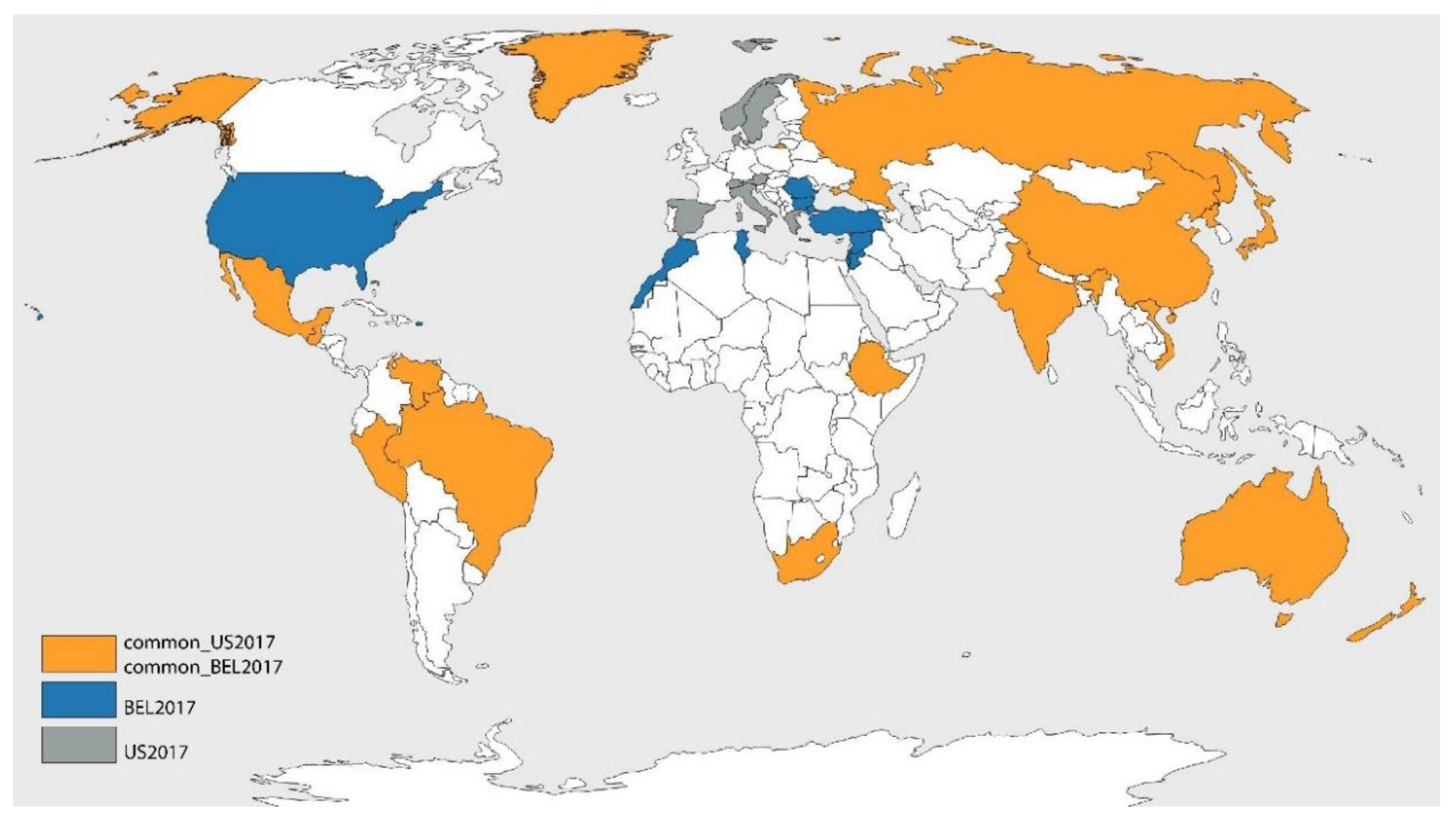
To make valid comparisons between the Belgian and American participants, the datasets with the common test regions were used: common_BEL2017 and common_US2017. Nevertheless, note that the reference regions are not the same for both groups, so the results of the comparisons are indicative.

The study reveals that Belgian students estimate more accurately the real size of test regions compared to American students. This could be explained by their broader knowledge about cartography with more specific map projections. Besides the estimation itself, the additional information about the confidence of the estimation and the answers on personal characteristics of the students is analyzed as well. The American students answered significantly more positively than the Belgian students on the question ‘Can you locate this country or continent on a world map?’ However, this neither results in more certainty about their answers nor in more accurate estimates.

The questionnaire provided interesting material regarding the use of the Internet and web maps and the cartographic knowledge of the participating students. All the students used the Internet daily, while the use of social media was slightly higher in Belgium than in the US. In addition, 9% of the American students claimed to never use these media. 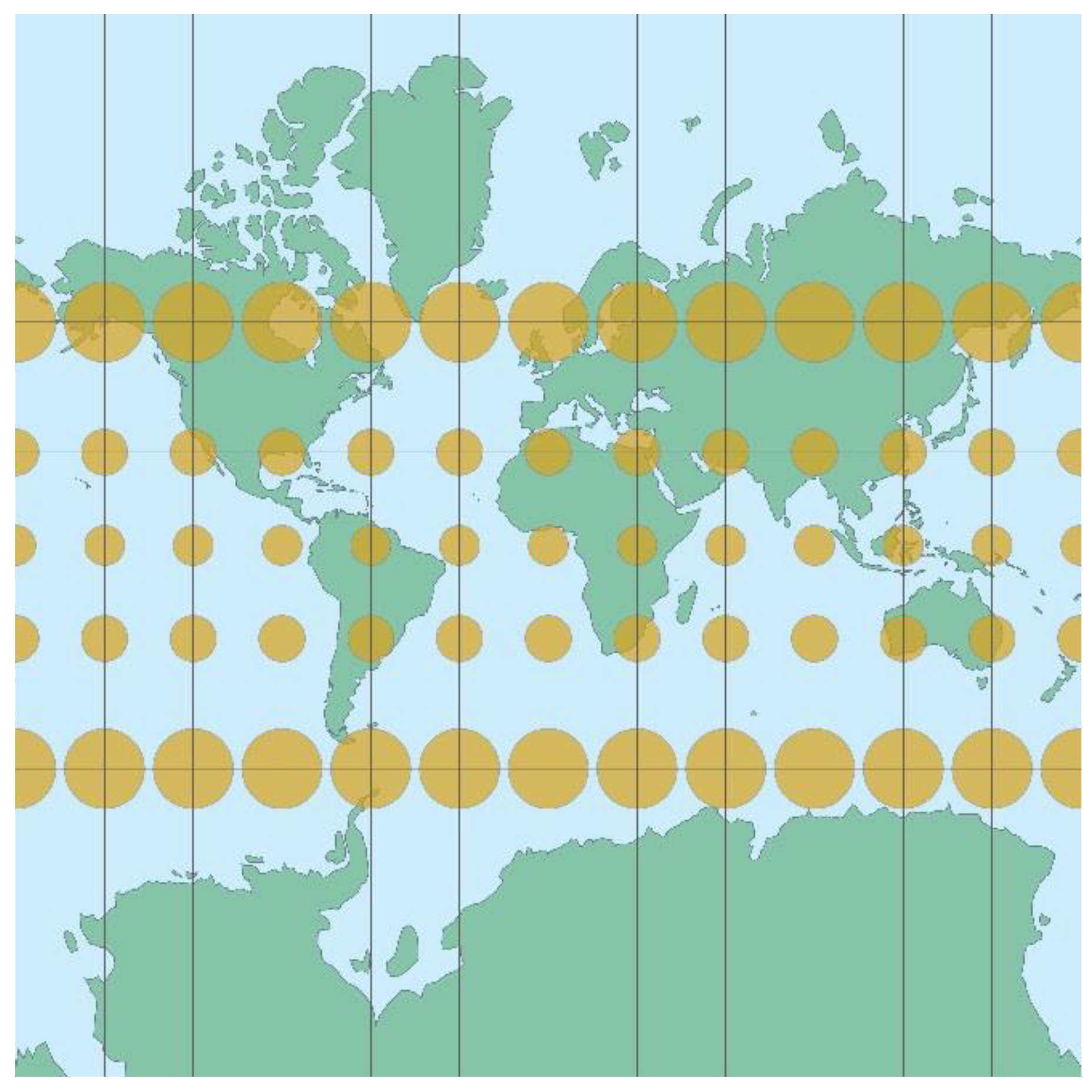This does not match the global statistics that state that 76% of the US population and 66% of the Belgian population use Facebook and other social media (http://gs.statcounter.com/social-media-stats). This discrepancy was probably the result of the small number of participants and an inaccurate representation of the national population of both countries. Regarding the knowledge of cartography, the Belgian students stated a greater familiarity with cartography and map projections. This knowledge resulted in more students being familiar with the Mercator map distortions.

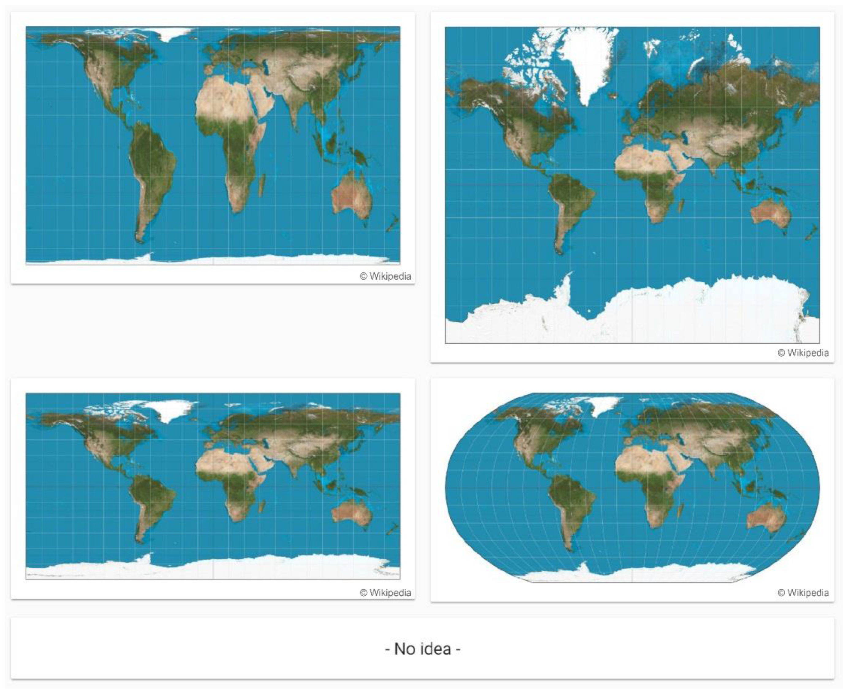
Consequently, more Belgian students selected the Gall-Peters projection as an equal-area projection. Still, one-third of American students were aware of the Mercator map distortions as well. This can be triggered by the recent debate about the use of map projections in the education system that has been in the media [52,53,54,55,56]. Despite 72% of the American students not selecting the Gall-Peters projection as an equal area, only 55% of the Belgian students considered the Gall-Peters projection as a non-equal-area, which is in line with the findings of Battersby and Kessler [57]. In their study, 51% of the participants wrongly indicated that this projection distorts area. For the Gall-Peters projection, the distorted shape of regions was a crucial factor to evaluate this map as a distorted area. 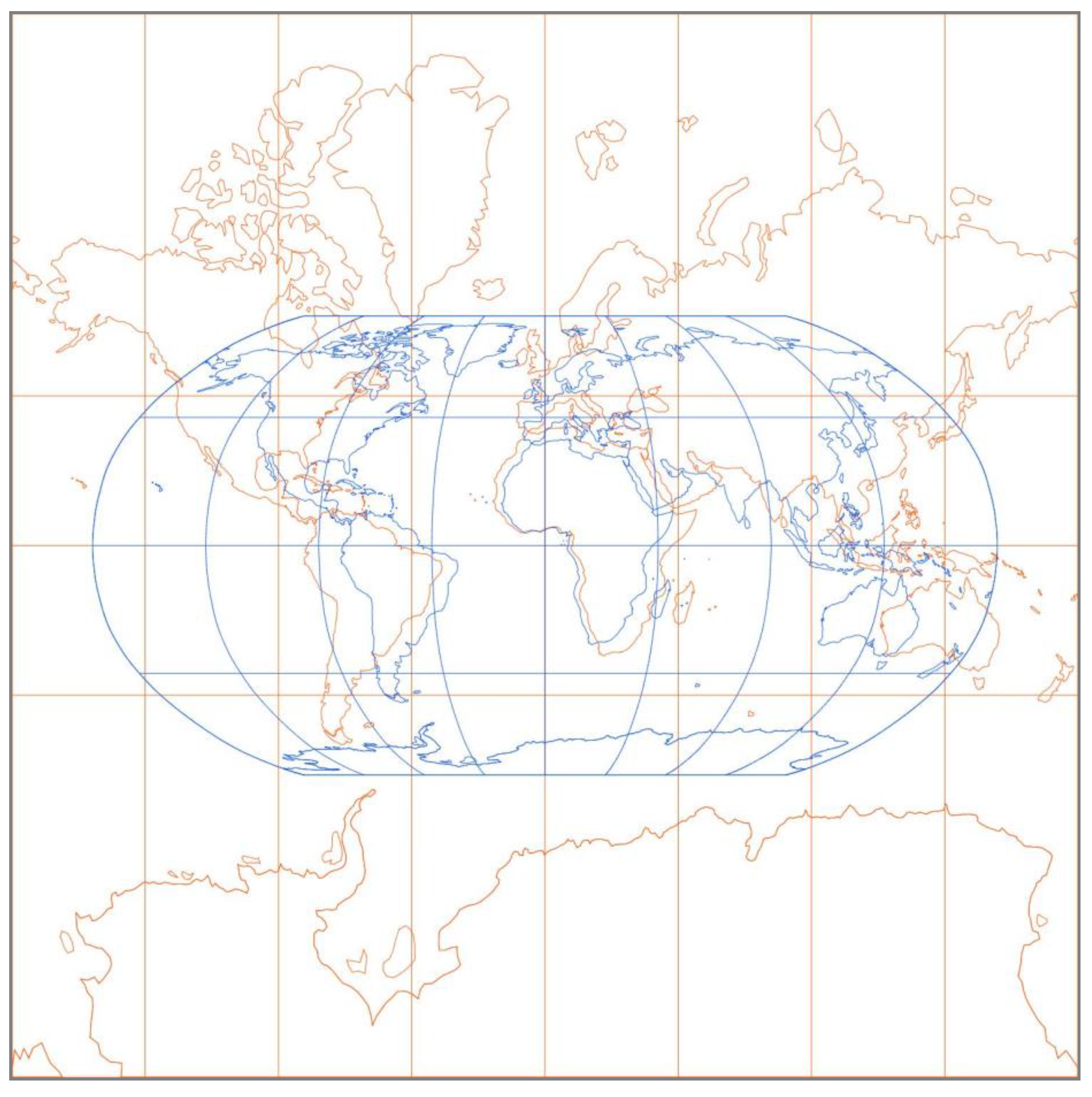Furthermore, Battersby and Kessler [57] discovered that the Robinson projection is considered the least distorted projection and is probably encountered as what MacEachren [58] refers to as a ‘map schema’—a general mental image of a global-scale map. These findings correspond with our results that both American and Belgian students acknowledge the Robinson projection as the most familiar. This familiarity could be a result of the shape of the countries and regions that are considered not distorted. Second, the Robinson projection is still widespread in Belgium, as well as in the US [57], since it was selected as the primary map projection by the National Geographic Society from 1988 until 1998 and since then has been applied for several purposes such as for education in textbooks and in atlases as world map projection (e.g., De Boeck atlas). Currently, other, similar-looking, compromised map projections are common in education or the media. For example, the Winkel-Tripel and Van Grinten map projections (e.g., Plantyn Algemene Wereldatlas, Collins World Atlas, and New Concise World Atlas). It is noticeable that the students were more familiar with a compromised map projection than with the Web Mercator projection utilized by web maps, such as Google Maps. These web maps are used frequently by young people but possibly mostly as a navigational instrument and, therefore, on a local scale and not a global level, such as the global maps in atlases.

4.2. Differences over Time: Between 2006 and 2017

Several scientists claim that repeatedly being exposed to the (Web) Mercator projection—such as while watching or analyzing map mashups with Google maps as the background—can result in a deformation of people’s mental map [24,26]. When this deformation is comparable to the distortions of the (Web) Mercator map projection, this is called the Mercator effect. The study of Battersby and Montello from 2006 did not reveal any proof for the existence of the Mercator effect [47]. With the development of web maps beginning in 2005 and the widespread use of social media, people use and share more data and (thematic) maps. Therefore, the question arises whether the present generation of adolescents, who grew up amid these technological developments, are more influenced by the (Web) Mercator map. The results of this study, completed in 2017, did not provide any other conclusions than the preceding research of 2006. No proof for the Mercator effect could be found. Moreover, the results of US2006 and US2017 are remarkably similar. There are, in general, only very small differences between the 2006 and 2017 datasets. Nevertheless, the mean estimated areas of US2017_country are systematically and significantly higher than those of US2006. The difference between the β-values of the two power functions confirm this as well because a higher β-value corresponds with larger estimates and, in this case, larger overestimations. The reason for this phenomenon is not clear. It is also reflected in the normalized values of the relative estimated accuracy. These values are, for every test region, higher in 2017 than in 2006. However, the differences between the relative estimated accuracy of the two groups is not significant. The normalization of the data seems to lessen the differences between the two datasets.

4.3. Recommendations for Further Research

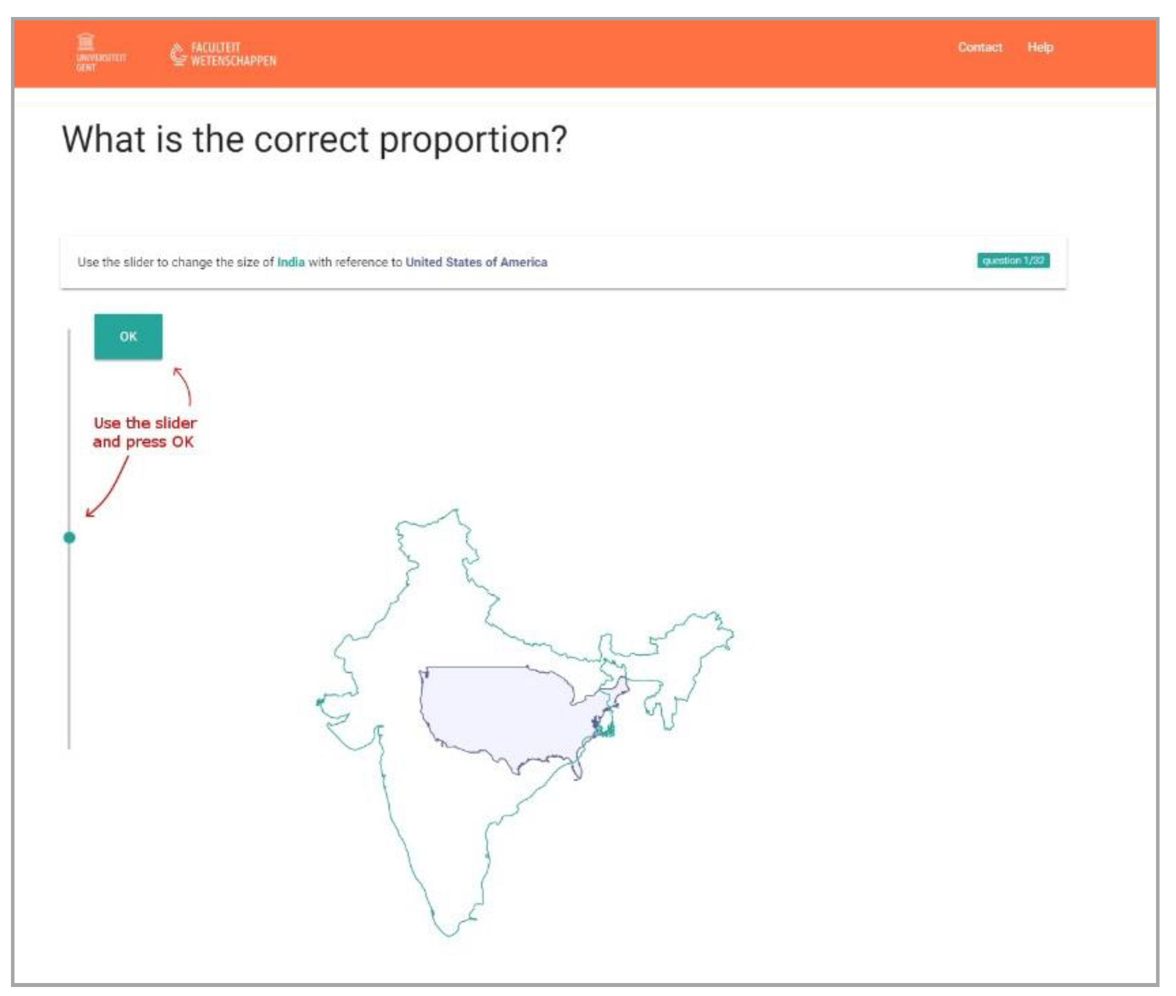
This study should be considered a preliminary study from which the initial conclusions can be drawn and serves as an input prior to the development of a more extensive and global study, which involves more participants and countries worldwide. As in every research project, this project inherently has some limitations. In particular, this research is built upon an existing study from 2006. Ideally, the setup ought to be identical to the original version developed by Battersby and Montello. Since the original version could not be re-used, some restrictions were applied regarding the programming of the tool, such as the minimum and maximum estimations and the selection of the countries.

The fixed size of the reference region resulted in a limited maximum estimation of a test region, which can be important for the estimation of large countries or continents. Therefore, the fixed size of the reference region (for BEL2017 and US2017) was set as the value, while the Mercator area of the largest country, Russia, could be doubly overestimated. Battersby and Montello used a maximum and minimum size for each test region separately, based on the results of their previous study (‘Numerical magnitude area estimation from memory’) [27]. This distinction in setup caused a size difference of the reference region presented on the screen. The disadvantage of this was that the reference regions for BEL2017 and US2017 were represented as smaller on the screen than for US2006. This might be a possible reason why smaller countries of US2017 were systematically more overestimated compared to the US2006 study.

Moreover, the selection of test regions should preferably be identical to the previous study of 2006. While this was straightforward for the US2017 study, it was not possible for the Belgian version of the test, since Europe was selected as the reference region. Therefore, several smaller European countries could not be included in the Belgian list of test regions. To obtain a comparable group of test regions, there were two factors to consider. The two factors are the size and the latitude of the countries. Due to the exceptionally high concentration of small countries in Europe, it became impossible to exchange the small European countries of US2006 with other small countries at the same latitude. Therefore, small countries located around Europe were selected. These countries include Bulgaria, Israel, Jordan, Morocco, Romania, Syria, Tunisia, and Turkey. Consequently, this selection resulted in a low number of mutual countries for comparing the two study groups (common_US2017 and common_BEL2017), which makes the concluding comparisons less strong and valid.

To conclude, further research that scales both the test and reference region would be a valuable improvement. This would allow for the selection of any possible comparison between the two regions. Another possibility is to eliminate the use of one reference region and provide comparisons of two test regions. Consequently, no countries would need to be excluded from the selected list of countries. All of them could be combined with another except in the case that they are neighboring countries. This would allow for the collection of data from anywhere in the world without needing to change the reference region in favor of the participating nationalities. Moreover, gathering personal data, such as migration, travelling countries, and cartographical background, could result in a better visualization of the reference region. Rotating a set of test regions minimizes these influential factors.

In addition, collecting data in two different countries makes the selection of the participants even more precarious. Besides age, another determinant factor is educational background and knowledge about map projections. Not only do the name of the educational programs between countries differ but also their content and even the prior knowledge or cultural customs, such as the use of the Internet, paper, and web maps. To collect these details about the participants, the questionnaire was extensive.

Nevertheless, it can be concluded that the variation of participants is considerable and could possibly influence the analysis. However, this limitation could be solved in the future by focusing on a broader target group and collecting data from more participants. Therefore, it is necessary to adjust the test in such a way that it is more attractive such as by making it shorter, increasing the usability, or adding a playful element. Likewise, a more extensive questionnaire that inquires about participants’ affinity with particular countries—places where participants have family or friends, that they have visited frequently, or that they frequently saw in their school books or in the news—could provide good measures for further analysis of the collected data.

Attempting to eliminate differences between this study and the 2006 study caused some setup limitations. However, this shed light on recommendations for further research. In sum, providing the participants with the possibility to scale both the test and reference region could be a valuable improvement. Another option is to eliminate the use of one reference region and provide comparisons of two test regions.

5. Conclusions

To identify the impact of the use of web maps on a cognitive map, an online test was developed that asked young people to estimate the real proportions of some regions. Students of the US and Belgium who grew up amid the development of web maps and social media participated in this research. It is assumed that they are more influenced by these web maps and its Web Mercator projection than the students of the US who participated in 2006 at the advent of such technological development. Battersby and Montello [47] did not discover any Mercator effect in their research. However, many researchers suggest the existence of a Mercator effect [23,24,26], and some of them found indications [34,59,60]. Still, there is much speculation. Therefore, the fundamentals of the test developed in 2006 [47] were reused and redesigned in a new online test in which students of the US participated. Students of Belgium were included as well but in an adapted version of the test. This allowed us to evaluate the evolution between American students of 2006 and 2017 but also to test for intercontinental differences.

Although this study could not identify any evidence for the existence of a Mercator effect, the collected data provided some valuable insight into the cartographical background of the young people of Belgium and the US and how they estimate areas. For example, the certainty rate reveals that, in general, students are not very confident in estimating the size of regions, presumably because it is a difficult assignment. While completing it, people invoke their own image of the world to try to estimate the size as best as they can. Of course, this recalled image of the world is influenced by many known and unknown factors, such as education, use of the Internet and web maps, maps in the media, travel experiences, cultural and migration background, interests of parents, and more. The results of this research demonstrate that the use of web maps is probably less influential than the maps used in the educational system since most students indicate being most familiar with the Robinson map projection. This fact combined with a strong relationship between the reality and the estimates indicate that the participants are aware of the real proportions of the countries and continents. Since this study experienced some limitations regarding the selection of participants and reference and test regions, it would be interesting to develop a short, attractive online test that can easily be shared with several Internet users. The more people who participate, the more valid the results would be. In addition, a larger pool of country combinations and combinations of continents would make the cultural or migration background of the participant less influential.

References

1. Cartwright, W. Neocartography: Opportunities, Issues and Prospects. S. Afr. J. Geomat. 2012, 1, 14–31. [Google Scholar]
2. Gale, G. Push Pins, Dots, Customisation, Brands and Services: The Three Waves of Making Digital Maps. Cartogr. J. 2013, 50, 155–160. [Google Scholar] [CrossRef]
3. Haklay, M.; Singleton, A.; Parker, C. Web mapping 2.0: The neogeography of the GeoWeb. Geogr. Compass 2008, 2, 2011–2039. [Google Scholar] [CrossRef]
4. Peterson, M.P. Mapping in the Cloud; Guilford Press: New York, NY, USA, 2014; p. 421. [Google Scholar]
5. Turner, A.J. Introduction to Neogeography; O’Reilly Media, Inc.: Sebastopol, CA, USA, 2006; Volume 54. [Google Scholar]
6. Batty, M.; Hudson-Smith, A.; Milton, R.; Crooks, A. Map mashups, Web 2.0 and the GIS revolution. Ann. Gis 2010, 16, 1–13. [Google Scholar] [CrossRef]
7. Field, K. Maps, mashups and smashups. Cartogr. J. 2008, 45, 241–245. [Google Scholar] [CrossRef]
8. Hudson-Smith, A.; Crooks, A.; Gibin, M.; Milton, R.; Batty, M. NeoGeography and Web 2.0: Concepts, tools and applications. J. Locat. Based Serv. 2009, 3, 118–145. [Google Scholar] [CrossRef]
9. Muehlenhaus, I. Web Cartography—Map Design for Interactive and Mobile Devices; Taylor and Francis Group: Boca Raton, FL, USA, 2014; p. 230. [Google Scholar]
10. Ooms, K.; De Maeyer, P.; Dupont, L.; Van Der Veken, N.; Van de Weghe, N.; Verplaetse, S. Education in Cartography: What is the Status of Young People’s Map-Reading Skills? Cartogr. Geogr. Inf. Sci. 2015, 43, 1–20. [Google Scholar] [CrossRef]
11. Tsou, M.-H. Revisiting Web Cartography in the United States: The Rise of User-Centered Design. Cartogr. Geogr. Inf. Sci. 2011, 38, 250–257. [Google Scholar] [CrossRef]
12. Battersby, S.E. Distortion of Area in the Global-Scale Cognitive Map—A Geographic Perspective; University of California: Santa Barbara, CA, USA, 2006; p. 217. [Google Scholar]
13. Battersby, S.E.; Finn, M.P.; Usery, E.L.; Yamamoto, K.H. Implications of Web Mercator and Its Use in Online Mapping. Cartogr. Int. J. Geogr. Inf. Geovis. 2014, 49, 85–101. [Google Scholar] [CrossRef]
14. Çöltekin, A.; Garlandini, S.; Heil, B.; Fabrikant, S.I. Evaluating the Effectiveness of Interactive Map Interface Designs: A Case Study with Eye Movement Analysis. In Proceedings of the AutoCarto 2008, Sherpherdstown, WV, USA, 8–11 September 2008; pp. 1–12. [Google Scholar]
15. Das, T.; van Elzakker, C.P.J.M.; Kraak, M.-J. Conflicts in Neogeography Maps. In Proceedings of the AutoCarto 2012, Columbus, OH, USA, 16–18 September 2012; p. 14. [Google Scholar]
16. Ooms, K.; De Maeyer, P.; Fack, V.; Van Assche, E.; Witlox, F. Investigating the effectiveness of an efficient label placement method using eye movement data. Cartogr. J. 2012, 49, 234–246. [Google Scholar] [CrossRef]
17. Roth, R.E. Challenges for Human Subjects Research in Cartography. In Proceedings of the ICA Workshop on Envisioning the Future of Cartographic Research, Curitiba, Brazil, 21 August 2015. [Google Scholar]
18. van Elzakker, C.P.J.M. The Use of Maps in the Exploration of Geographic Data; Utrecht University: Utrecht, The Netherlands, 2004; p. 208. [Google Scholar]
19. Brainerd, J.; Pang, A. Interactive map projections and distortion. Comput. Geosci. 2001, 27, 299–314. [Google Scholar] [CrossRef]
20. Šavrič, B.; Jenny, B. A new pseudocylindrical equal-area projection for adaptive composite map projections. Int. J. Geogr. Inf. Sci. 2014, 28, 2373–2389. [Google Scholar] [CrossRef]
21. Canters, F.; Decleir, H. The World in Perspective: A Directory of World Map Projections; John Wiley & Sons Ltd.: Hoboken, NJ, USA, 1989; p. 181. [Google Scholar]
22. Monmonier, M.S. Rhumb Lines and Map Wars: A Social History of the Mercator Projection; University of Chicago Press: Chicago, IL, USA, 2004; p. 256. [Google Scholar]
23. Monmonier, M. Lying with Maps. Stat. Sci. 2005, 20, 215–222. [Google Scholar] [CrossRef]
24. Wood, D.; Kaiser, W.L.; Abramms, B. Seeing through Maps: Many Ways to See the World; New Internationalist Publications Ltd.: Oxford, UK, 2006; p. 152. [Google Scholar]
25. Monmonier, M.S. How to Lie With Maps, 2nd ed.; University of Chicago Press: Chicago, IL, USA, 1996; p. 207. [Google Scholar]
26. Robinson, A.H. Rectangular World Maps—No. Prof. Geogr. 1990, 42, 101–104. [Google Scholar] [CrossRef]
27. Battersby, S.E. The Effect of Global-Scale Map-Projection Knowledge on Perceived Land Area. Cartogr. Int. J. Geogr. Inf. Geovis. 2009, 44, 33–44. [Google Scholar] [CrossRef]
28. Battersby, S.E. Map projection and global-scale spatial cognition. In Proceedings of the International Conference of Cartography 2005, Coruña, Spain, 9–16 July 2005. [Google Scholar]
29. Downs, R.; Stea, D. Maps in Minds. Reflection on Cognitive Mapping; Harper & Row: New York, NY, USA, 1977; p. 205. [Google Scholar]
30. Keates, J.S. Understanding Maps; Addison Wesley Longman Limited: Harlow, UK, 1996; p. 334. [Google Scholar]
31. Tversky, B. Distortions in cognitive maps. Geoforum 1992, 23, 131–138. [Google Scholar] [CrossRef]
32. Monmonier, M. Cartography: Distortions, world-views and creative solutions. Prof. Geogr. 2005, 29, 217–224. [Google Scholar] [CrossRef]
33. King, R.; Vujaković, P. Peters Atlas: A new era of cartography or publishers con-trick? Geography 1989, 74, 245–251. [Google Scholar]
34. Saarinen, T.; Parton, M.; Billberg, R. Relative Size of Continents on World Sketch Maps. Cartographica 1996, 33, 37–48. [Google Scholar] [CrossRef]
35. Vujakovic, P. Damn or be damned: Arno Peters and the Struggle for the ‘New Cartography’. Cartogr. J. 2003, 40, 61–67. [Google Scholar] [CrossRef]
36. Vujaković, P. Mapping the World Development. Geography 1989, 74, 97–105. [Google Scholar]
37. Lloyd, R. Self-Organized Cognitive Maps. Prof. Geogr. 2000, 52, 517–531. [Google Scholar] [CrossRef]
38. Roth, R.; Ross, K.; MacEachren, A. User-Centered Design for Interactive Maps: A Case Study in Crime Analysis. Isprs Int. J. Geo-Inf. 2015, 4, 262–301. [Google Scholar] [CrossRef] [Green Version]
39. Skarlatidou, A.; Haklay, M. Public web mapping: Preliminary usability evaluation. In Proceedings of the Geographical Information Science Research Conference 2006, Nottingham, UK, 6–8 April 2006. [Google Scholar]
40. Schobesberger, D. Integrating User and Usability Research in Web-Mapping Application Design. In Modern Trends in Cartography; Brus, J., Vondrakova, A., Vozenilek, V., Eds.; Springer International Publishing: Basel, Switzerland, 2015; pp. 147–158. [Google Scholar]
41. van Elzakker, C.P.J.M.; Delikostidis, I.; van Oosterom, P.J.M. Field-Based Usability Evaluation Methodology for Mobile Geo-Applications. Cartogr. J. 2008, 45, 139–149. [Google Scholar] [CrossRef]
42. Slocum, T.A.; Blok, C.; Jiang, B.; Koussoulakou, A.; Montello, D.R.; Fuhrmann, S.; Hedley, N.R. Cognitive and Usability Issues in Geovisualization. Cartogr. Geogr. Inf. Sci. 2001, 28, 1–28. [Google Scholar] [CrossRef]
43. van Elzakker, C.P.J.M.; Griffin, A.L. Focus on geoinformation users: Cognitive and use/user issues in contemporary cartography. Gim Int. 2013, 27, 20–23. [Google Scholar]
44. Montello, D.R. Cognitive Map-Design Research in the Twentieth Century: Theoretical and Empirical Approaches. Cartogr. Geogr. Inf. Sci. 2002, 29, 283–304. [Google Scholar] [CrossRef]
45. Fabrikant, S.I.; Lobben, A. Introduction: Cognitive Issues in Geographic Information Visualization. Cartographica 2009, 44, 5. [Google Scholar] [CrossRef]
46. MacEachren, A.M.; Kraak, M.-J. Research Challenges in Geovisualization. Cartogr. Geogr. Inf. Sci. 2001, 28, 3–12. [Google Scholar] [CrossRef]
47. Battersby, S.E.; Montello, D.R. Area Estimation of World Regions and the Projection of the Global-Scale Cognitive Map. Ann. Assoc. Am. Geogr. 2009, 99, 273–291. [Google Scholar] [CrossRef]
48. Lapon, L.; Ooms, K.; De Maeyer, P. The influence of the Web Mercator projection on the global-scale cognitive map of web map users. In Proceedings of the Workshops and Posters at the 13th International Conference on Spatial Information Theory (COSIT 2017), l’Aquila, Italy, 4–8 September 2017. [Google Scholar]
49. Lapon, L.; Ooms, K.; De Maeyer, P.; Dupont, L.; De Wit, B.; Vanhaeren, N. The influence of web maps and education on adolescents’ global-scale cognitive map. Cartogr. J. Publication under review.
50. Moore, D.S.; McCabe, G.; Craig, B.A. Introduction to the Practice of Statistics; W.H. Freeman and Company: New York, NY, USA, 2009; p. 709. [Google Scholar]
51. Cohen, J. Applied Multiple Regression/Correlation Analysis for the Behavioral Sciences, 3rd ed.; Erlbaum: Mahwah, NJ, USA, 2003; p. 736. [Google Scholar]
52. Boston Public Schools Map Switch Aims to Amend 500 Years of Distortion. Available online: https://www.theguardian.com/education/2017/mar/19/boston-public-schools-world-map-mercator-peters-projection (accessed on 31 January 2019).
53. Boston Schools Have Introduced a New World Map—But It’s Just as Wrong as the One Your’re Familiar with. Available online: https://www.businessinsider.com/boston-school-gall-peters-map-also-wrong-mercator-2017-3?r=UK (accessed on 31 January 2019).
54. Why Map Historians Are Annoyed With Boston Public Schools. Available online: https://www.atlasobscura.com/articles/mercator-peters-boston-map (accessed on 31 January 2019).
55. Will Boston’s Switch from Mercator Maps Leave Kids Asking ‘Where in the World Is…’? Available online: https://www.dw.com/en/will-bostons-switch-from-mercator-maps-leave-kids-asking-where-in-the-world-is/a-38051003 (accessed on 31 January 2019).
56. Scholen in Boston Bekijken de Wereld Vanuit een Nieuw Perspectief. Available online: https://www.vrt.be/vrtnws/nl/2017/03/21/scholen_in_bostonbekijkendewereldvanuiteennieuwperspectief-1-2930015/ (accessed on 31 January 2019).
57. Battersby, S.E.; Kessler, F.C. Cues for Interpreting Distortion in Map Projections. J. Geogr. 2012, 111, 93–101. [Google Scholar] [CrossRef]
58. MacEachren, A. How Maps Work. Representation, Visualization, and Design; The Guildford Press: New York, NY, USA, 1995; p. 513. [Google Scholar]
59. Saarinen, T. The Euro-Centric Nature of Mental Maps of the World. Res. Geogr. Educ. 1999, 1, 136–178. [Google Scholar]
60. Chiodo, J.J. Improving the Cognitive Development of Students’ Mental Maps of the World. J. Geogr. 1997, 96, 153–163. [Google Scholar] [CrossRef]
Figure 1. The Tissot’s indicatrices visualized the Mercator map projection and its local distortions. Source: FlexProjector.
Ijgi 08 00125 g001
Figure 2. The Mercator projection (in orange) compared to the Robinson projection (in blue). Source: FlexProjector.
Ijgi 08 00125 g002
Figure 3. The interface of the online test, with India as test region on top of reference region the conterminous United States, shows the initial sizes of the regions. The width of the test region is twice the size of the reference region.
Ijgi 08 00125 g003
Figure 4. Overview of the test regions on a world map, projected with Winkel Tripel map projection, which is the standard of the National Geographical Society since 1998 (orange: the common regions for US (common_US2017) and Belgian studies 2017 (common_BEL2017), blue: additional regions for 2017 study Belgium (BEL2017), grey: additional regions for 2017 study US (US2017).
Ijgi 08 00125 g004
Figure 5. Illustration of the four map projections represented in the test.
Ijgi 08 00125 g005
Figure 6. Power function of BEL2017 (left) and US2017 (right).
Ijgi 08 00125 g006