Article

Voxel-based 3D Point Cloud Semantic Segmentation: Unsupervised Geometric and Relationship Featuring vs Deep Learning Methods

Geomatics Unit, University of Liège (ULiege), Allée du six Août, 19, 4000 Liège, Belgium
*
Author to whom correspondence should be addressed.
ISPRS Int. J. Geo-Inf. 2019, 8(5), 213; https://0-doi-org.brum.beds.ac.uk/10.3390/ijgi8050213
Submission received: 6 March 2019 / Revised: 11 April 2019 / Accepted: 3 May 2019 / Published: 7 May 2019

Abstract

:
Automation in point cloud data processing is central in knowledge discovery within decision-making systems. The definition of relevant features is often key for segmentation and classification, with automated workflows presenting the main challenges. In this paper, we propose a voxel-based feature engineering that better characterize point clusters and provide strong support to supervised or unsupervised classification. We provide different feature generalization levels to permit interoperable frameworks. First, we recommend a shape-based feature set (SF1) that only leverages the raw X, Y, Z attributes of any point cloud. Afterwards, we derive relationship and topology between voxel entities to obtain a three-dimensional (3D) structural connectivity feature set (SF2). Finally, we provide a knowledge-based decision tree to permit infrastructure-related classification. We study SF1/SF2 synergy on a new semantic segmentation framework for the constitution of a higher semantic representation of point clouds in relevant clusters. Finally, we benchmark the approach against novel and best-performing deep-learning methods while using the full S3DIS dataset. We highlight good performances, easy-integration, and high F1-score (> 85%) for planar-dominant classes that are comparable to state-of-the-art deep learning.

Graphical Abstract

1. Introduction

Extracting knowledge from raw point cloud data is actively driving academic and industrial research. There is a great need for automated processes that can speed up and make existing frameworks faster and more reliable. It often integrates a classification step to extract any relevant information regarding one application domain. However, one classification approach cannot efficiently satisfy all of the domains as the semantic concepts that are attached to objects and the location can vary, depending on uses (e.g., considering a chair as an object, or its legs). Therefore, ensuring that such information is transferable to benefit other applications could provide a great opening on point cloud data usage. Yet, this is a non-trivial task that necessitates highly interoperable reasoning and a flexible way to handle data, relationships, and semantics. Our method considers the Gestalt’s theory [1], which states that the whole is greater than the sum of its parts, and that relationships between the parts can yield new properties/features. We want to leverage the human visual system predisposition to group sets of elements.
In this paper, the first goal is to provide a point cloud parsing unit to extract the semantic clusters through a voxel-based partitioning of the dataset. It permits flexible usage in different domains, such as Architecture, Engineering, and Construction (AEC), Building Information Modelling (BIM), Facility Management (FM), indoor navigation, and robotics. The module acts as a standalone within a Smart Point Cloud Infrastructure [2]—a set-up where point data is the core of decision-making processes—and it handles point clouds with heterogeneous characteristics. Indeed, the possibility to incorporate Knowledge-Extraction routines in existing frameworks has become essential for an efficient international research cooperation for the sake of interoperable data management. As such, we investigate an objective solution for versatile 3D point cloud semantic representation transparent enough to be usable on different point clouds and within different application domains. We propose to structure a point cloud in Connected Elements that is further refined in Semantic patches using efficient and low-level voxel-related features. This is primarily motivated by the limitations of point-based approach, where the amount of data, the redundancy, and the absence of relationships within points are great performance issues.
In order to assess the possibilities given by the 3D clustering scheme, a semantic segmentation solution is developed to leverage feature sets that retain both shape and relationship information. This permit benchmarking the performances and results against the best-performing state of the art deep-learning methods. Indeed, with the rise in computing power, promising machine learning techniques, as detailed in [3,4,5,6,7,8,9,10,11,12,13,14,15], are a great opening to more reliable and robust 3D objects classification. However, ground-truth extraction and dataset labelling to create training data are the main drawbacks in supervised learning. Manually annotating and ensuring the quality of such datasets is a heavily dauting task. Hence, ways to alleviate these mechanisms through automated tools are essential for new findings and in training new models.
The experiments were conducted on the full S3DIS [16] indoor dataset as (e.g., Figure 1), but it is generalizable to outdoor environments with man-made objects/characteristics.
Briefly, this paper makes the following three main contributions:
  • a new interoperable point cloud data clustering approach that account variability of domains for higher-end applications;
  • a novel point cloud voxel-based featuring developed to accurately and robustly characterize a point cloud with local shape descriptors and topology pointers. It is robust to noise, resolution variation, clutter, occlusion, and point irregularity; and,
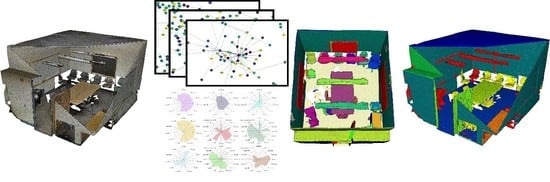
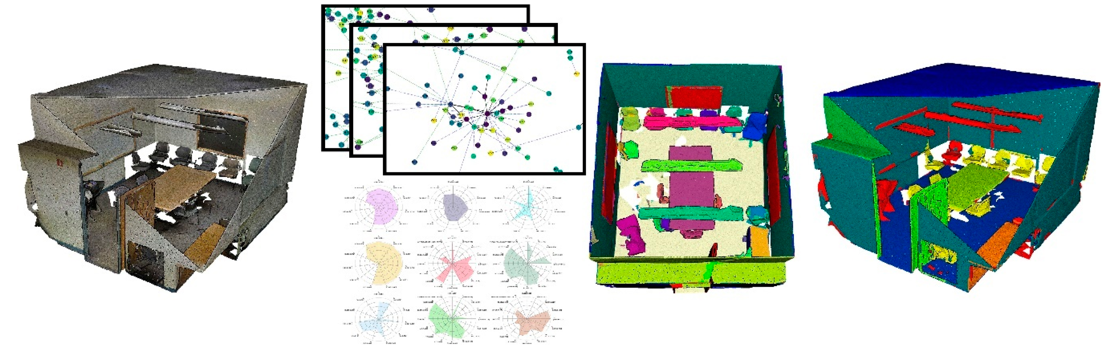
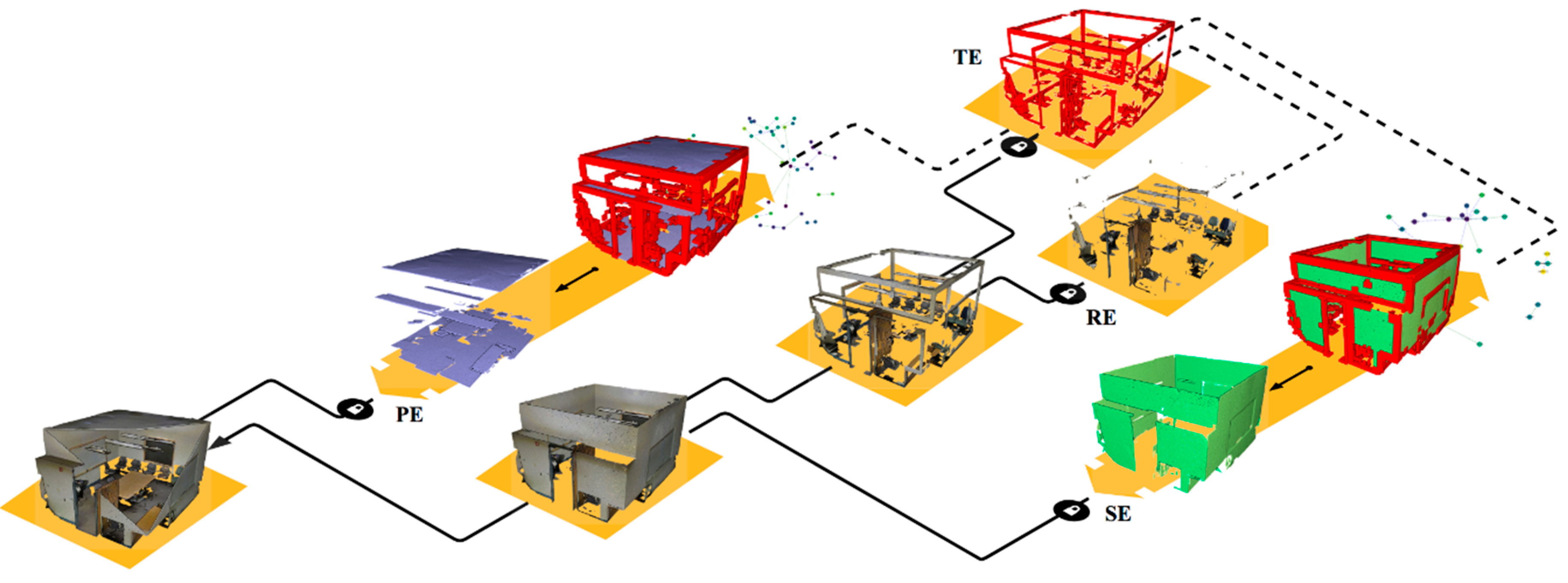
  • a semantic segmentation framework to efficiently decompose large point clouds in related Connected Elements (unsupervised) that are specialized through a graph-based approach: it is fully benchmarked against state-of-the-art deep learning methods. We specifically looked at parallelization-compatible workflows.
The reminder of this paper is structured, as follows. Section 2 briefly reviews recent related works dealing with point cloud feature extraction, segmentation, and classification. Section 3 gives the details of the proposed voxel-based featuring and semantic segmentation. In Section 4, we present the S3DIS dataset that is used for the different experiments and benchmarks. In Section 5, we study the impact of features over the results and analyse the performance of the approach against high-yielding supervised learning. In Section 6, we discuss our findings and highlight limitations as research directions.

2. Related Works

Feature design occupies a central position in knowledge representation and classification approaches. As expressed in Section 1, the Gestalt’s theory [1] is fundamental to understand how our visual cognition systems perceive our surrounding when trying to feed a classifier with information. It is often very hard to translate the factors into algorithms, while many of them make intuitive sense (e.g., Figure 2).
This gives an edge to deep learning approaches, where the emphasis is toward training the dataset’s constitution rather than feature engineering. In this section, we cover both problematics, i.e., feature- engineering and point-cloud supervised learning, which is further linked to Section 3 and Section 5. First, the features and methods that work well for extracting relevant information from point clouds are investigated. Subsequently, relevant references and recent works (2015+) that deal with point clouds semantic segmentation are given to the reader. We specifically look at voxel approaches and features that already made their proof over complex point cloud artefacts.

2.1. Point Cloud Feature Extraction

In this sub-section, we analyse low-level shape-based approaches that try to extract local descriptors from the 3D neighbourhood [17]. We refer initially to the pertinent work of Ghorpade et al. [18], which proposes a review of two-dimensional (2D) and 3D shape representation and it is a good introduction to obtaining an idea of the landscape of features in use.
The work of Bueno et al. [19] focuses on the detection of geometric key-points and its application to point cloud registration. The authors primarily study data subsampling to keep the key points for coarse alignment purposes. These points are obtained using an approach that is mainly based on the features of eigen entropy, change of curvature, and planarity. Indeed, they state that these provide a good representation in both, visual, and mathematical value of the point clouds. This is found in many recent works, such as [20,21], where authors also use local eigen-based features for disaster damage detection through synergistic use of deep learning. The work of Blomley et al. [22] provides larger insights on the common geometric (e.g., eigen-based) covariance features in varying scale scenarios. In 2018, Thomas et al. proposed a semantic classification of 3D point clouds in [8], which also employs eigen-based features as well as colour derived feature. The specificity lies in the definition of a multiscale neighbourhoods, which allows for the computation of features with a consistent geometrical meaning. The authors in [23] also uses several eigen-based feature, spectral and colour-derived features for the classification of aerial LiDAR point clouds. The features, coupled with their approach, provide good results, and therefore orient our choice of features toward eigen-based features, for they are representative of local neighbourhood as well as low-knowledge requirement.
Other recent works for learning local structures [24] or local shape properties [14] highlighted the wide acceptation of normals. In [24], Shen et al. present two new operations to improve PointNet [25]—one of the earliest deep learning reference for point cloud semantic segmentation—with a more efficient exploitation of local structures. The first one focuses on local 3D geometric structures. In analogy to a convolution kernel for images, they define a point-set kernel as a set of learnable 3D points that jointly respond to a set of neighbouring data points according to their geometric affinities, as measured by kernel correlation. The second one exploits local high-dimensional feature structures by recursive feature aggregation on a nearest-neighbour-graph computed from 3D positions. They specifically state that “As a basic surface property, surface normals are heavily used in many areas including 3D shape reconstruction, plane extraction, and point set registration” [26,27,28,29,30]. The paper of Song et al. [31] provides a comparison of normal estimation methods, which can also be achieved via neural networks, such as PCPNet [14]. In this last article, Guerrero et al. propose a deep-learning method for estimating the local 3D shape properties in point clouds. The approach is especially well-adapted for estimating local shape properties, such as normals (both unoriented and oriented) and curvature from raw point clouds in the presence of strong noise and multi-scale features. Therefore, we will specifically integrate normal within our workflow, while looking at performance issues during its computation.
Edge-based features have also been investigated in [32] or [33], but their applicability is mostly oriented toward point cloud line tracing. Thus, we confront large performance issues due to analysing geometric properties of each point’s neighbourhood, and combining RANSAC [34,35] and angular gap metrics to detect the edges. While extended in [36] to contour the extraction of large 3D point clouds, we will specifically avoid region growing approaches due to performance limitations.

2.2. Semantic Segmentation Applied to Point Clouds

The first challenge in pure segmentation frameworks is to obtain group of points that can describe with the organization of the data by a relevant clustering enough detachment. The work of Papon et al. have provided the first approach of using relationships while conserving the point-based flexibility [32]. They propose an over-segmentation algorithm using ‘supervoxels’, an analogue of the superpixel approach for 2D methods. Based on a local k-means clustering, they try and group the voxels with similar feature signatures (39-dimensional vector) to obtain segments. The work is interesting because it is one of the earliest to try and propose a voxel-clustering with the aim of proposing a generalist decomposition of point cloud data in segments. Son et Kim use such a structure in [37] for indoor point cloud data segmentation. They aim at generating the as-built BIMs from laser-scan data obtained during the construction phase. Their approach consists of three steps: region-of-interest detection to distinguish the 3D points that are part of the structural elements to be modelled, scene segmentation to partition the 3D points into meaningful parts comprising different types of elements while using local concave and convex properties between structural elements, and volumetric representation. The approach clearly shows the dominance of planar features in man-made environments.
Another very pertinent work is [38], which proposes a SigVox descriptor. The paper first categorizes object recognition task following the approach of: (1) model-fitting based (starts with segmenting and clustering point cloud, followed by fitting point segments); (2) semantic methods (based on a set of rule-based prior knowledge); and, (3) shape-based methods (shape featuring from implicit and explicit point clusters). They use a 3D ‘EGI’ descriptor to differentiate voxels that only extract specific values from a Principal Component Analysis (PCA) [39]. The approach proves useful for MLS point clouds, grouping points in object candidates, following the number. Another voxel-based segmentation approach is given in [40,41] while using a probabilistic connectivity model. The authors use a voxel structure, in which they extract local contextual pairwise-connectivity. It uses geometric “cues” in a local Euclidean neighbourhood to study the possible similarity between voxels. This approach is similar to [42], where the authors classify a 2.5D aerial LiDAR point cloud multi-level semantic relationships description (point homogeneity, supervoxel adjacency, class-knowledge constraints). They use a feature set, among others, composed of the elevation above ground, normal vectors, variances, and eigen-based features. Another analogous approach can be found in [43] for building point detection from vehicle-borne LiDAR data based on voxel group and horizontal hollow analysis. Authors present a framework for automatic building point extraction, which includes three main steps: voxel group-based shape recognition, category-oriented merging, and building point identification by horizontal hollow ratio analysis. This article proposes a concept of “voxel group”, where each group is composed of several voxels that belong to one single class-dependent object. Subsequently, the shapes of point clouds in each voxel group are recognized and this shape information is utilized to merge the voxel group. This article efficiently leverages a sensory characteristic of vehicle-borne LiDAR building data but specializes the approach in consequence.
The references [44,45] are built upon a graph-based over-segmentation methodology that is composed of a local 3D variation extraction, a graph construction, descriptor computation, and edge-wise assignment, followed by sequential subgraph criteria-based merging. The used descriptors are mainly RGB, location and normal vectors on top of the fast point feature histogram [46]. While the approach is domain-related, it offers some additional insight regarding the power of relational approaches between local point patches for the task of semantic segmentation. However, as shown in [10], using a multi-scale voxel representation of 3D space is very beneficial, even in complexity reduction of terrestrial lidar data. The authors propose a combination of point and voxel generated features to segment 3D point clouds into homogenous groups in order to study the surface changes and vegetation cover. The results suggest that the combination of point and voxel features represent the dataset well, which shows the benefit of dual representations. The work of [17] uses Random Forests for aerial Lidar point cloud segmentation, which aims at extracting planar, smooth, and rough surfaces, being classified using semantic rules. This is interesting to answer specific domains through ontology formalization.
These methodologies contrast with deep learning approaches, as they try to solve the semantic segmentation problem by first understanding which set of features/relations will be useful to obtain the relevant results. The following methodologies directly start with the data and will learn by themselves how to combine the initial attributes (X, Y, Z, R, G, B…) into efficient features for the task at hand. Following PointNet [25] and PointNet++ [47], which are considered as a baseline approach in the community, other work applied deep learning to point set input or voxel representations.
The end-to-end framework SEGCloud [48] combines a 3D-FCNN, trilinear interpolation, and CRF to provide class labels for 3D point clouds. Their approach is mainly performance-oriented when compared to state-of-the-art methods that are based on neural networks, random forests, and graphical models. Interestingly, they use a trilinear interpolation, which adds an extra boost in performance, enabling segmentation in the original 3D points space from the voxel representation. Landrieu and Simonovsky provide another promising approach for large scale Point Cloud semantic segmentation with Superpoint graphs [49]. In the article, the authors propose a deep learning-based framework for semantic segmentation of point clouds. They initially postulate that the organization of 3D point clouds can be efficiently captured by a structure (Superpoint graph), which is derived from a partition of the scanned scene into geometrically homogeneous elements. Their goal is to offer a compact representation of the contextual relationships between object parts to exploit through convolutional network. In essence, the approach is similar to [2,50], through a graph-based representation. Finally, the works of Engelmann et al. in [12,51] provides very interesting performances by including the spatial context into the PointNet neural network architecture [51] or providing an efficient feature learning and neighbourhood selection strategy [12]. These works are very inspiring, and they have the potential to become de-facto methodologies for a wide variety of application through transfer learning. As such, they comprise very good methodologies for benchmarking semantic segmentation approaches.
We highlighted three different directions that will drive our methodology in this state-of-the-art review of pertinent related work. First, it is important that we identify the key points in a point cloud that can retain a relevant connotation to domain-related objects. Secondly, we noted that, for gravity-based scenes, these elements have a space continuity and often feature homogeneity. Third, specifically, man-made scenes retain a high proportion of planar surfaces that can host other elements (floor, ceiling, wall …) [52]. Therefore, detecting these constitutes a central first step in our methodological framework, but they must be quick, scalable, robust, reliable, and flexible. It is important to note that the global context may be lost if working with relatively small neighbourhood samples.

3. Materials and Methods

In this section, we describe a point cloud parsing method to extract semantic clusters (Connected Elements [50]), which can be refined in application-dependent classes.
Our automatic procedure is serialized in seven steps, as illustrated in Figure 3 and described in the four following sub-sections. In Section 3.1, we describe the voxel grid constitution. In Section 3.2, we cover feature extraction processes for low-level shape descriptors (Section 3.2.1) and relational features (Section 3.2.2). Subsequently, in Section 3.3 we provide a connected-component system using extracted feature sets SF1 and SF2, followed by a point-level refinement within each voxel to obtain Semantic patches. Finally, we propose a graph-based assembly for the constitution of Connected Elements [2] and a classification routine to obtain labelled point data (Section 3.4) benchmarked in Section 5.

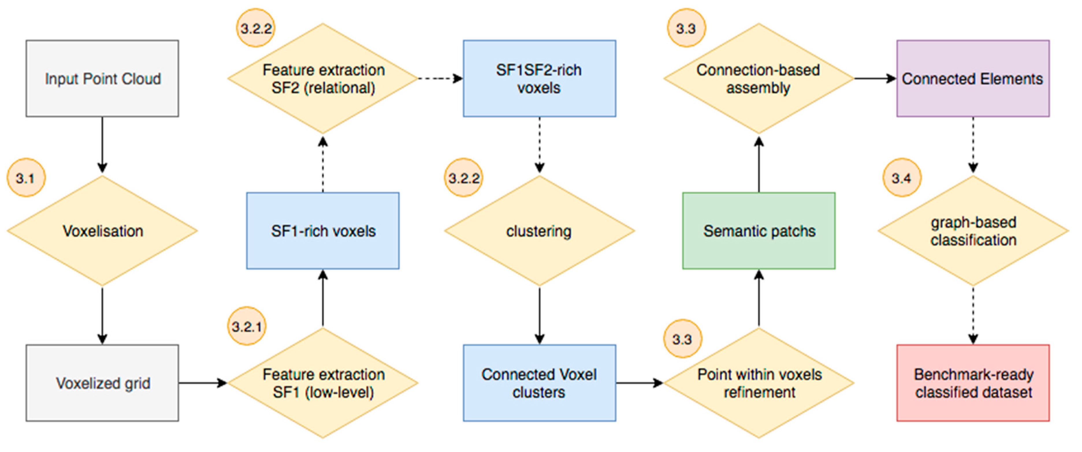
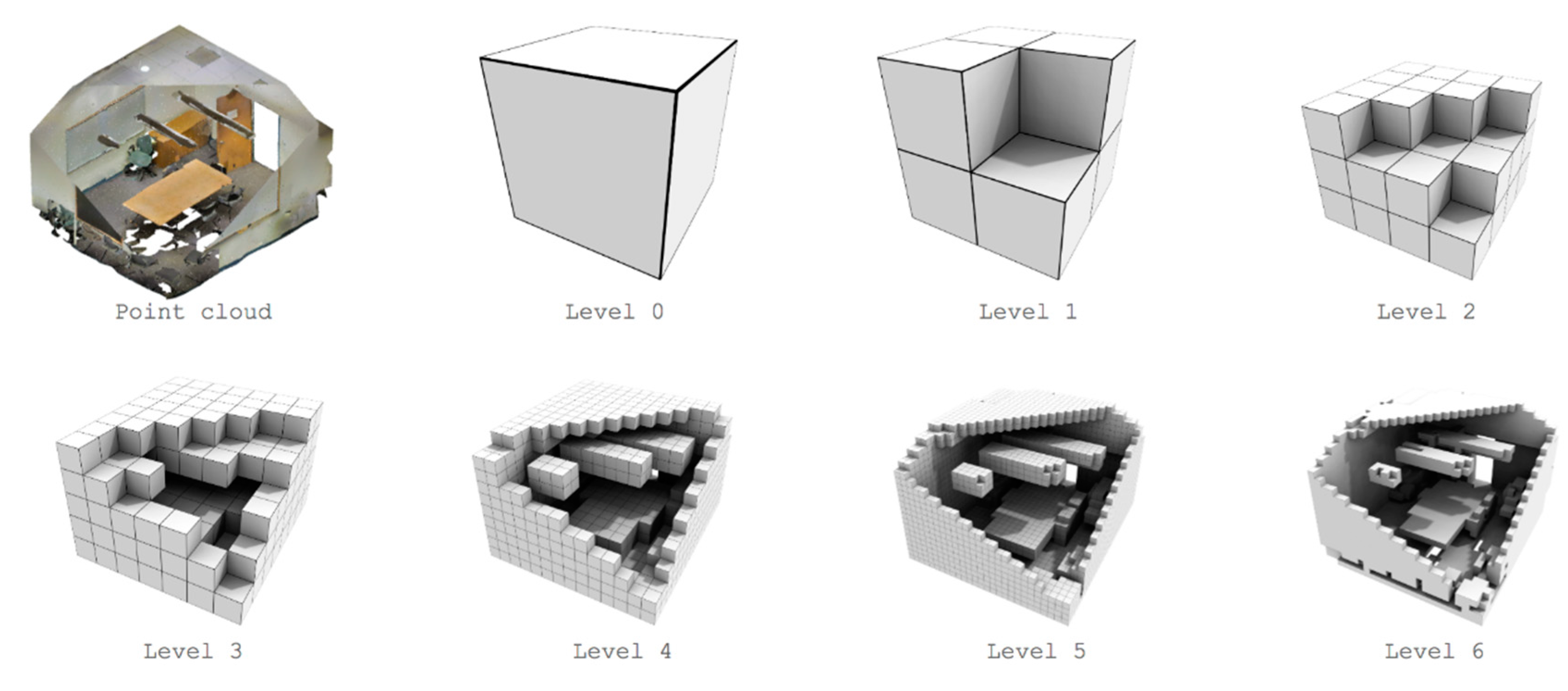
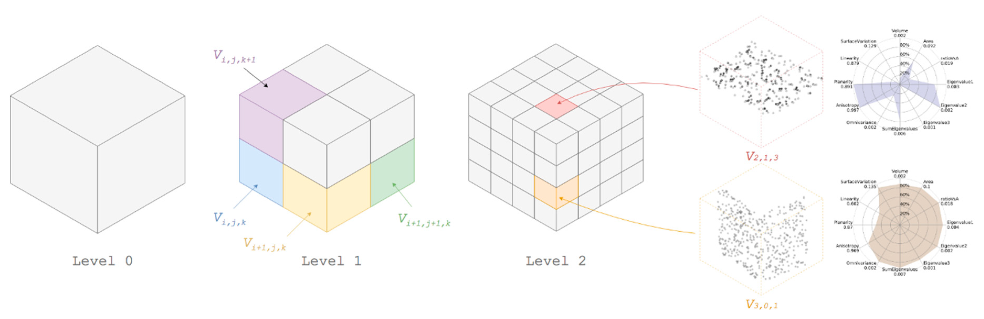
3.1. Voxelisation Grid Constitution

Our approach proposes integrating different generalization levels in both feature space and spatial space. First, we establish an octree-derived voxel grid over the point cloud and we store points at the leaf level. As stated in [53,54,55], an octree involves recursively subdividing an initial bounding-box into smaller voxels until a depth level is reached. Various termination criteria may be used: the minimal voxel size, predefined maximum depth tree, or a maximum number of sample points within a voxel. In the proposed algorithm, a maximum depth tree is used to avoid the computations necessitating domain knowledge early on. We study the impact of tree depth selection over performances in Section 5, starting at a minimum level of 4 to study the influence of the design choice. The grid is constructed following the initial spatial frame system of the point cloud to account for complex scenarios where point repartition does not precisely follow the axes.
Let p i be a point in s , with s the number of dimensions. We have a point cloud P = { p i } i = 1 n with n the number of points in the point cloud. Let V i , j , k be a voxel of P identified by a label L i , containing m points from P .
The cubic volume, defined by a voxel entity, provides us with the advantage of fast yet uniform space division, and we hence obtain an octree-based voxel structure at a specific depth level. Our approach, similarly to [56], is constructed using indexes to avoid overhead. The constituted voxel grid, with the goal of creating Connected Elements discards, empty voxels to only retain points-filled voxels. However, for higher end applications, such as pathfinding, the voxel-grid can be used as a negative to look for empty spaces. Subsequently, we construct a directed graph , defined by a set v ( ) of inner nodes, a set ( ) of edges, and a set v e ( ) of leaf nodes, with each representing a non-empty voxel at an octree level, illustrated over a room sample of the S3DIS dataset in Figure 4.
Once each point has been assigned to a voxel regarding the defined grid within the 3 Euclidean space along e x ,   e y ,   e z , we consider the leaf nodes v e ( ) of as our representative primitive.

3.2. Feature Extraction

We aim at extracting a robust feature set for general semantic segmentation frameworks, as a single object of the resulting feature vector is hardly interpretable [57]. To insure interoperable workflows, we used descriptors that were thoroughly studied and made their proof in various works referred in Section 2.
Our new voxel-primitive serves as an initial feature host, and it acts as a point neighbourhood selection approach. These can then be transferred following the structure of , permitting feature transfer at every octree depth level extended to the point-storage (Figure 5).
This permits a flexible and unconstrained feature-based point cloud parsing, which can process raw data (i.e., pure X, Y, Z Euclidean sets). In the next Section 3.2.1, we present several low-level shape-based features that are used to construct our SF1 feature set. Afterwards, we explain our relationship-level feature set (SF2) that permits leveraging local topology and relationships at different cluster levels.

3.2.1. Low-Level Shape-Based Features (SF1)

The first group of low-level features is mainly derived from Σ , our data covariance matrix of points within each voxel for the low memory footprint and fast calculation, which, in our case, we define as:
Σ = 1 m 1 i = 1 m ( X i X ¯ ) ( X i X ¯ ) T
where X ¯ is the mean vector X ¯ = i = 1 m p i .
From this high yielding matrix, we derive eigen values and eigen vectors through Singular Value Decomposition [58] to increase the computing efficiency, which firstly correspond to modelling our voxel containment by a plane, showing to largely improve performances. We follow a Principal Component Analysis (PCA) to describe three principal axes describing the point sample dispersion. Thus, we rely heavily on eigen vectors and eigen values as a feature descriptor at this point. Therefore, their determination needs to be robust. This is why we use a variant of the Robust PCA approach presented in the article [59] to avoid miscalculation. We sort eigenvalues λ 1 ,   λ 2 ,   λ 3 , such as λ 1 > λ 2 > λ 3 , where linked eigen vector v 1 ,   v 2 ,   v 3 , respectively, represent the principal direction, its orthogonal direction, and the estimated plane normal. These indicators, as reviewed in Section 2, are interesting for deriving several eigen-based features [23], as following:
λ a = ( λ 1 λ 3 ) / λ 1
λ l = ( λ 1 λ 2 ) / λ 1
λ p = ( λ 2 λ 3 ) / λ 1
λ v = λ 3 / i = 1 3 λ i
λ o = i = 1 3 λ i 3
λ s = λ 3 / λ 1
λ e = i = 1 3 λ i ln ( λ i )
where for the voxel V i , j , k , λ a is its anisotropy, λ l its linearity, λ p its planarity, λ v its surface variation, λ o its omnivariance, λ s its sphericity, and λ e its eigen entropy. Table 1 summarizes the first set of eigen-based features.
We extract a second geometry-related set of features (Table 2), starting with V i x ¯ ,   V i y ¯ ,   V i z ¯ the mean value of points within a voxel V i , j , k .
The area features V A p ,   V A are obtained through a convex hull (Equation (10)) analysis, respectively, along v 3 and e z . The third is the local point density within the segment, which is defined as follows:
D V = m V V
where V V is the minimum volume calculated through a 3D convex hull, such as:
C o n v ( P ) = { i = 1 | P | α i q i | ( i : α i 0 ) i = 1 | P | α I = 1 }
V V = 1 3 | j = 1 m ( Q F . n F ) a r e a ( F ) |
We standardize their values from different dynamic ranges into a specified range, in order to prevent outweighing some attributes and to equalize the magnitude and variability of all features. There are three common normalization methods, as referred in [10]: Min-max, Z-score, and decimal scaling normalization. In this research, we use Min-max method that has been found to be empirically more computationally efficient in normalizing the multiple features F in F N , normalized feature in a [ 0 : 1 ] range:
F N = F min ( F ) max ( F ) min ( F )
We combine eigen-based features and geometrical features for easier data visualization in two separate spider charts (e.g., in Table 1 and Table 2). Subsequently, we plot normalized distributions per-voxel category (e.g., in Figure 6) to better understand the variations within features per element category.
We note that, for the example of Primary Elements (mostly planar, described in Section 3.3), there is a strong similarity within the global voxel feature sets, except for orientation-related features (Normals, Position, Centroids).

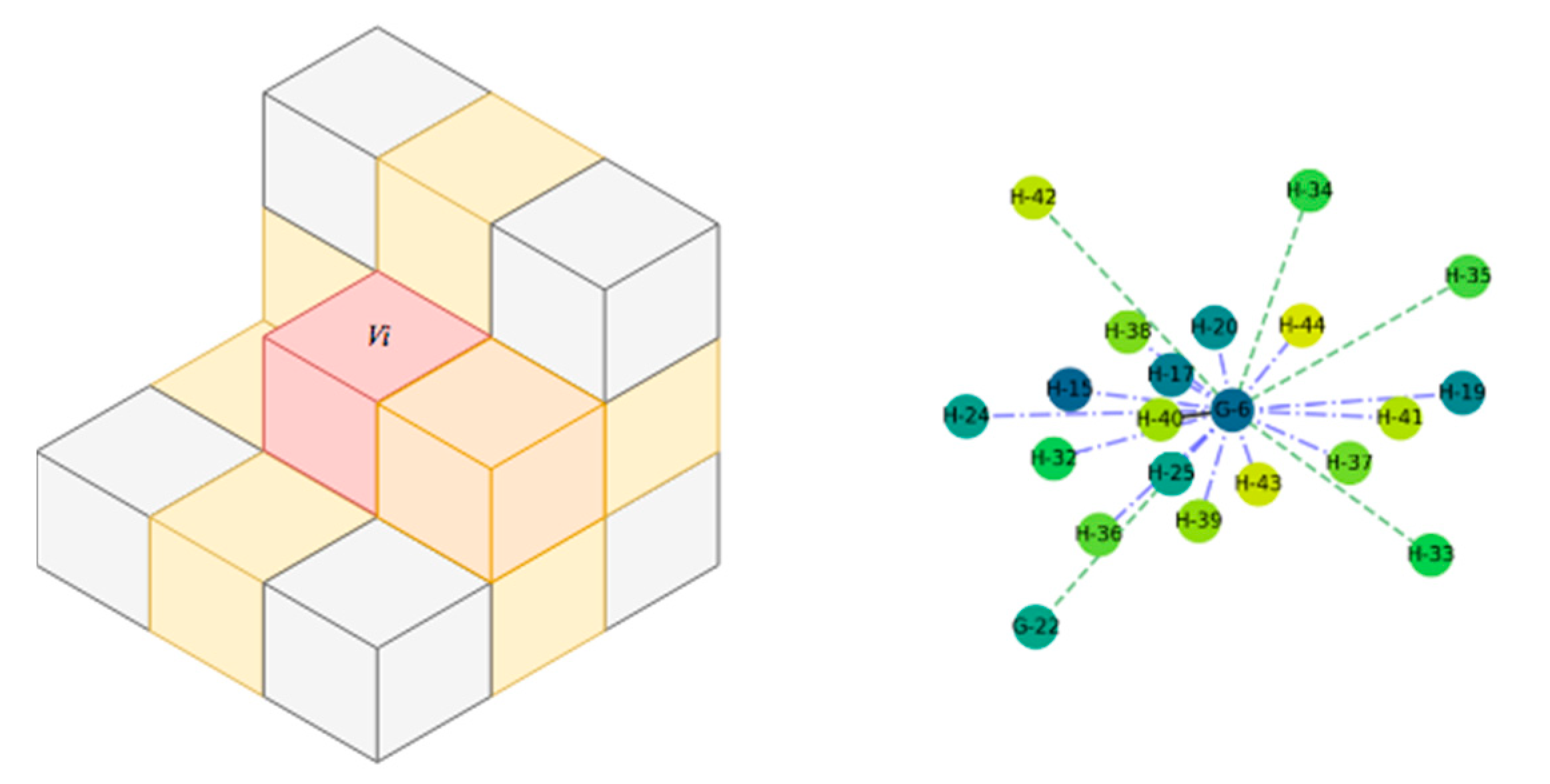
3.2.2. Connectivity and Relationship Features (SF2)

There are very few works that deal with explicit relationship feature extraction within point clouds. The complexity and exponential computation to extract relevant information at the point-level mostly justify this. Thus, the second set of proposed feature set (SF2) is determined at several octree levels. First, we extract a 26-connectivity graph for each leaf voxel, which appoints every neighbour for every voxel. These connectivity are primarily classified regarding their touch-topology [60], which either is vertex.touch, edge.touch, or face.touch (Figure 7).
Each processed voxel is complemented through new relational features to complement this characterization of voxel-to-voxel topology. Immediate neighbouring voxels are initially studied to extract F g (geometrical difference) while using the log Euclidean Riemannian metric, which is a measure of the similarity between adjacent voxels covariance matrices:
F g = log Σ v i log Σ v j F
where log(.) is the matrix logarithm operator and   . F is the Frobenius norm.
If the SF1 feature set is available (non-constrained through computational savings) and, depending on the desired characterization, these are favoured for an initial voxel tagging.
We estimate concavity and convexity between adjacent voxels to get higher end characterization while limiting the thread surcharge to a local vicinity. It refines the description of the graph edge between the processed node (voxel) and each of its neighbours (Algorithm 1). We define α V the angle between two voxels V i and V j , as:
α V = n V i ( Σ V i Σ V j )
Algorithm 1. Voxel Relation Convexity/Concavity Tagging
Require: A voxel V i and its direct vicinity { V j } j = 1 26 expressed as a graph .
1. For each V j do
2.   α V angle between normal of voxels
3.  if α V < 0 then
4.    i j ( ) edge between V i and V j is tagged as Concave
5.  else i j ( ) edge between V i and V j is tagged as Convex
6.  end if
7. end for
8. end
9. return ( )
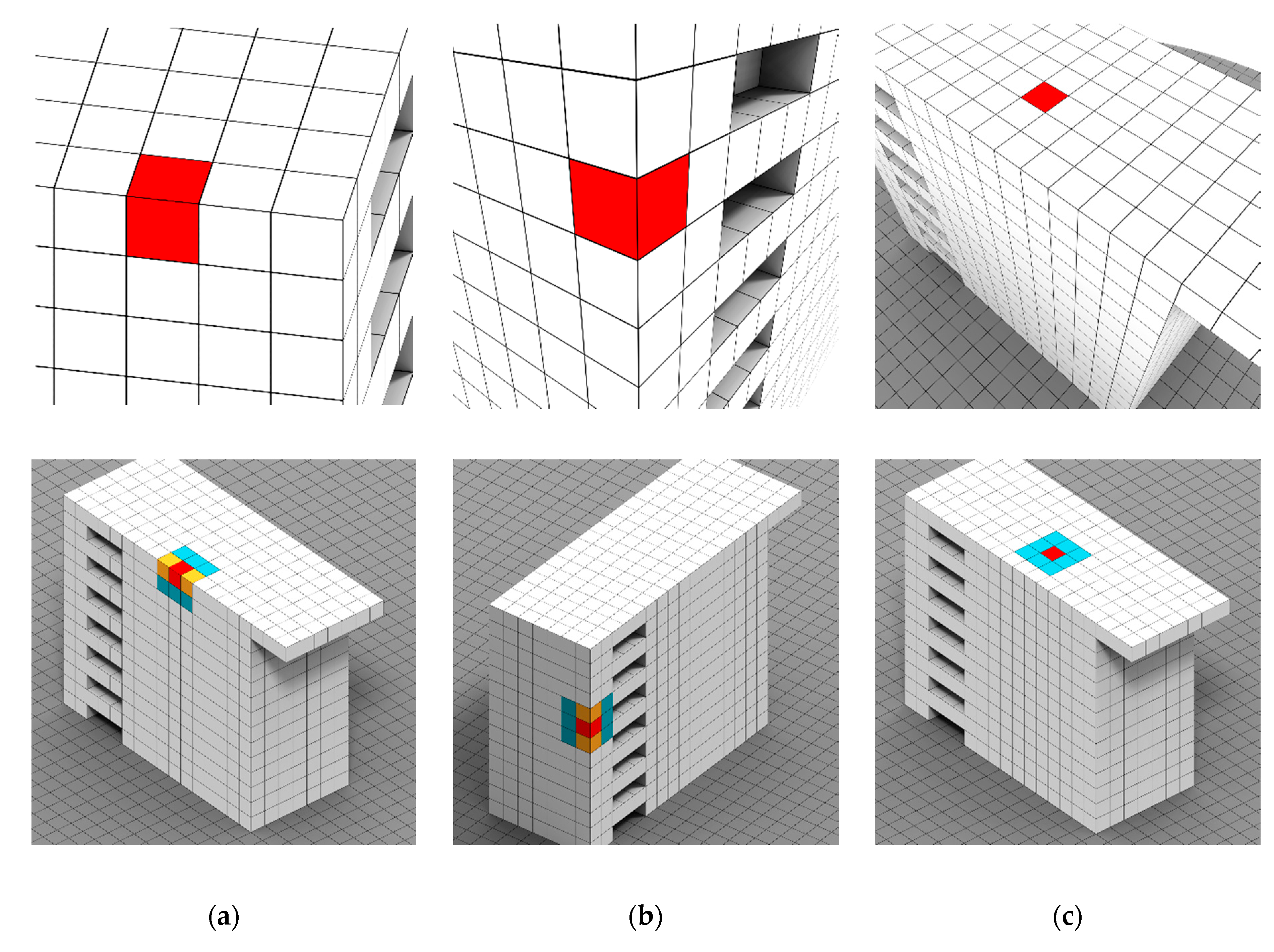
Third, we extract four different planarity-based relationships (Figure 8) between voxels, being:
  • Pure Horizontal relationship: For V i , if an adjacent voxel V j has a v 3 colinear to the main direction (vertical in gravity-based scenes), then the edge ( v i , v j ) is tagged H r . If two adjacent nodes v i and v j hold an H r relationship and both v 3 are not colinear, they are connected by a directed edge, d ( v i , v j ) , where v i is the starting node. In practice, voxels that are near horizontal surfaces hold this relationship.
  • Pure Vertical relationship: For V i , if an adjacent voxel V j has a v 3 orthogonal to the main direction (vertical in gravity-based scenes), then the edge ( v i , v j ) is tagged V . If two adjacent nodes v i and v j are connected through V r and both v 3 are coplanar but not colinear, then they are connected by a directed edge, d ( v i , v j ) . In the case that we are in a gravity-based scenario, they are further refined following v 1 and v 2 axis. These typically includes voxels that are near vertical surfaces.
  • Mixed relationship: For V i , if within its 26-connectivity neighbours, the node v i presents V and H r edges, then v i is tagged as M r . In practice, voxels near both horizontal and vertical surfaces hold this relationship.
  • Neighbouring relationship. If two voxels do not hold one of these former constraining relationships but are neighbours, then the associated nodes are connected by an undirected edge without tags.
Illustrated on the S3DIS dataset, Figure 9 is an example of the different voxel-categories:
Finally, the number of relationships per voxel is accounted as the edge weights pondered by the type of voxel-to-voxel topology, where vertex.touch = 1, edge.touch = 2, and face.touch = 3. We obtain a feature set SF2, as in Table 3:
This is translated into a multi-set graph representation to give a flexible featuring possibility to the initial point cloud. As such, extended vicinity is then a possible seed/host of new relationships that permit a topology view of the organization of voxels within the point cloud (e.g., Figure 10).
These relationships are represented in different groups to extract different features completing the relationship feature set. Graphs are automatically generated through full voxel samples regarding the Category tags and Convex-Concave tags.

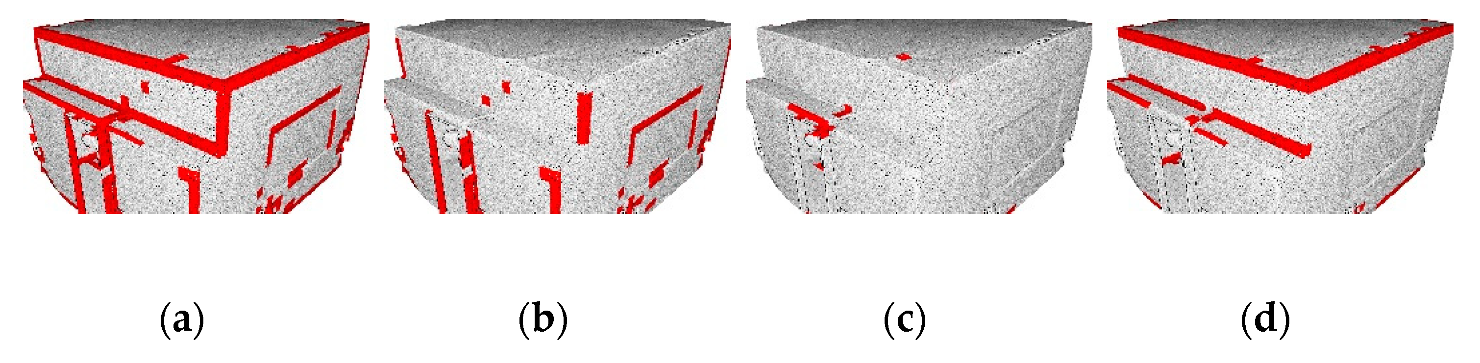
3.3. Connected Element Constitution and Voxel Refinement

Based on the feature sets SF1 and SF2, we propose a connected-component workflow that is driven by planar patches. Connected-component labelling is one of the most important processes for image analysis, image understanding, pattern recognition, and computer vision, and it is reviewed in [61]. Being mostly applied for 2D data, we extend it to our 3D octree structure for efficient processing and parallelization compatibility. We study the predominance of planar surfaces in man-made environments and the feature-related descriptor, which provides segmentation benefits. The designed feature representations that are described in Section 3.2 are used as a mean to segment the gridded point cloud into groups of voxels that share a conceptual similarity. These groups are categorized within four different entities: Primary Elements (PE), Secondary elements (SE), transition elements (TE), and remaining elements (RE), as illustrated in Figure 11.
We start by detecting the PE using both feature sets. Initially, we group the voxels that answer a collinearity condition with the main direction. This condition is translated by comparing the angle of normalized vectors against a threshold due to the normal dispersion in voxel sets (which has no exact collinear match):
α v < t h a         w i t h         α v = cos 1 ( v 3 ( i ) . v 3 ( j ) v 3 ( i ) . v 3 ( j ) )
We then cluster linked nodes through connected-component labelling using SF2. PE mainly presents clusters of points that are the main elements of furniture (table top, chair seat…) or ceiling and ground entities.
SE are constituted of voxels that hold v 3 orthogonal to the main direction, being further decomposed along v 1 and v 2 . As such, they are usually constituted of elements that belong to walls, and horizontal planar-parts of doors, beams …
The “edges” voxels that are within the set of tagged voxels { H r , V r , M r } are seeds to constitute TE, which are then further decomposed (voxel refinement) in semantic patches with homogeneous labelling, depending on their inner point characterization. As such, they play an important role in understanding the relationships between the primary, secondary, and remaining elements. They are initially grouped based on F g and clustered in connected-components using g 26 c c p ( i ) (SF2). The voxels containing “edges” (e.g., in Figure 12) or multiple possible points that should belong to separate objects are further subdivided by studying the topology and features with their neighbouring elements.
Finally, the remaining voxels are labelled through connected-components as RE, and their SF1-similarity is aggregated as a feature descriptor. For each element within the Connected Elements (CEL) set {PE, SE, TE, RE}, the voxel features are aggregated to obtain a global SF1 and SF2 feature set per CEL, being updated through voxel refinement. Implementation-wise, CEL are sorted by occupied volume after being sorted per category, Relationships exist between primary, secondary, edges, and remaining elements due to their voxel-based direct topology. This proximity is used to refine voxels (thus elements) by extracting points within voxel neighbours of an element ε i , which belongs to an element ε j based on defined SF1 features of ε i -voxel. This permit leveraging planar-based dominance in man-made scenes using, for example, eigen-based features. Thus, we extract a new connectivity graph between CEL where the weight of relationships is determined using the number of connected voxels. This allows for refining the transition voxels based on their local topology and connectivity to the surrounding elements. Therefore, the global element’s features play the role of reference descriptors per segment, and the points within targeted voxels for refinement are compared against these. If within voxel points justify belonging to another Connected Element, then the voxel is split in semantic patches, which each retains a homogeneous CEL label. The final structure retains unique CEL labels per leaf, where the leaves that are called semantic patches are either pure voxel or voxel’s leaf.
We obtain a graph-set composed of a general CEL graph, a PE graph, a SE graph, a TE graph, a RE graph, and any combination of PE, SE, TE, and RE (e.g., Figure 13):
We establish a graph-based semantic segmentation over these CEL in order to estimate the impact of designed features, as described in Section 3.4.

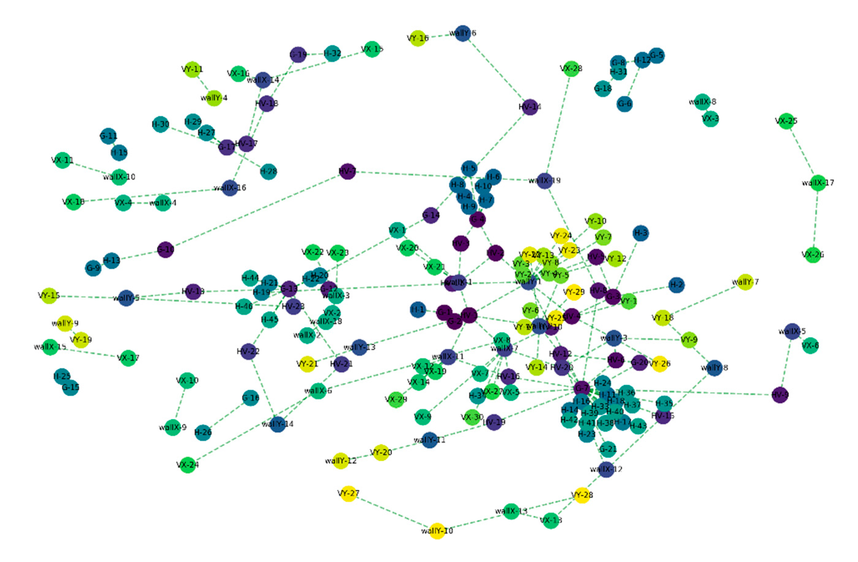
3.4. Graph-based Semantic Segmentation

We first employ a multi-graph-cut (set of edges whose removal makes the different graphs disconnected) approach depending on the weight of edges defining the strength of relations for every CEL in the graph-set, where the associated cut cost is:
c u t ( ε i , ε j ) = p ϵ ε i , q ϵ ε j w p q
where w p q is the weight of the edge between nodes p and q . We use normalized cut by normalizing for the size of each segment in order to avoid min-cut bias:
N c u t ( ε i , ε j ) = c u t ( ε i , ε j ) k ϵ e ε i ( g ) w k + c u t ( ε i , ε j ) k ϵ e ε j ( g ) w k
where e ε i ( g ) are the edges that touches ε i , and e ε i ( g ) are the edges that touches ε j .
Our approach was thought as a mean of only providing a first estimate of the representativity of CELs in semantic segmentation workflows, especially to differentiate big planar portions. As such, the provided classifier is very naïve, and it will be the subject of many improvements in the near future for better flexibility and to reduce empirical knowledge. It was constructed for indoor applications. For example, a segment with the largest membership to the ceiling might belong to beam or wall, and a segment with the largest membership to floor might belong to the wall or door. To handle such semantic mismatches, the graph g C E L , that was previously constructed is used to refine the sample selection using the following rules and the search sequence starting from the class floor, and it is followed by the class ceiling, wall, beam, table, bookcase, chair, and door. Once a node is labelled with one of these classes, it is excluded from the list of nodes being considered in the sample selection. The definition of thresholds was directly extracted from knowledge regarding the dimension of furniture objects from the European Standard EN1729-1:2015. As for the concepts at hand, these were defined regarding the Semantic Web resources, mainly the ifcOWL formalized ontology representing the Industry Foundation Classes application knowledge [62]. It is important to note that the furniture (chair, table, bookcases) models were extracted from these rules and we then simulated the scan positions to obtain simulated data. Indeed, sensors artefacts produce noisy point clouds, which can then slightly change the definition of thresholds. The obtained samples were then looked against five objects of the S3DIS to ensure consistency with the device knowledge.
(1) A node is tagged “floor” when for a primary element p ε i and all primary elements p ε :
V A ( p ε i ) m a x i m a s ( V A ( p ε ) )   &   k e p ε i ( g p ε ) m a x i m a s ( )   &   Z p ε i m a x i m a s ( Z p ε )
with k e p ε i ( g p ε ) being the sum of edge weights of all outgoing edges and incoming edges.
(2) The “ceiling” is similar to the “floor” labelling, with the difference that Z p ε i is searched among minimas of p ε .
(3) Once all of the ceiling and floor segments are identified, the nodes in the graph g s ε of secondary elements are searched for “wall” segments by first identifying all of the nodes that are connected to the ceiling or floor nodes through the edges of the designated relationships. The area feature guides the detection through thresholding to exclude non-maxima to handle complex cases.
(4) To identify “beams”, a sub-graph g r p ε s ε composed of remaining non-classified elements from PE and SE is generated. A connected-component labelling is performed guided by transition elements. It is then searched for nodes that are connected to the ceiling and the walls, which are then classified as “beam” segments.
(5) The “table” segments are extracted by the remaining elements of primary elements, if its SF1 feature set presents a correspondence of more than 50% with a sample table object. We note that the predominant factor is the height that is found within 70 and 110 cm from the ground segment. The feature correspondence is a simple non-weighted difference measure between the averaged SF1 features between the sample and the compared element. The sample element is constructed by following the domain concepts and thresholds, as explained previously.
(6) We identify “bookcases” if it presents a direct SF2 connectivity to wall segments and a SF1 feature correspondence of more than 50% from the remaining elements of RE.
(7) Subsequently, RE and remaining PE are aggregated through connected components and tagged as “chair” if their mean height above ground is under 100 cm.
(8) All of the unclassified remaining nodes are aggregated in a temporary graph and a connected-component labelling is executed. An element is tagged as “door” if the bounding-box element’s generalization intersect a wall segment.
(9) Every remaining element is classified as “clutter”.
By using the above nine rules, ceiling, floor, wall, beam, table, chair, bookcase, door, and clutter classes are looked for, going from raw point cloud to a classified dataset as illustrated in Figure 14.

4. Dataset

We evaluated feature performance in one application context to test our approach: 3D semantic segmentation for the indoor environment. We used the S3DIS dataset [16] from the Matterport sensor [63]. It is composed of six areas that are each subdivided in a specific number of rooms (Table 4) for a total of 270 sub-spaces [50]. These areas show diverse properties and include 156 offices, 11 conference rooms, two auditoriums, three lobbies, three lounges, 61 hallways, two copy rooms, three pantries, one open space, 19 storage rooms, and nine restrooms. One of the areas includes multiple floors, whereas the rest have one, and is very representative of building indoor spaces. The dataset is very noisy, presents imprecise geometries, clutter, and heavy occlusion. We noted that some points were mislabelled in the ground-truth labels during the tests, and that several duplicate points (points where the distance is inferior to 10−9 m from one another) add an extra bias. However, it was chosen, as it is a big dataset that provides a high variability of scene organization and it is currently used for benchmarking new algorithms. It is a very interesting opportunity to evaluate the robustness of our approach and to study the impact of features and their robustness to hefty point cloud artefacts. We remind the readers that the goal is to obtain relevant semantic patches constituting Connected Elements in a Smart Point Cloud Infrastructure.
We consider nine out of 13 classes in the S3DIS dataset, which hold 88.5% of the total number of segments representing both moveable and structural elements. The choice was motivated by the colour-dependence of the remaining classes. Indeed, in this article, we focus on a general approach with minimal input and, as such, we filtered the initial dataset before computing metrics for every point initially assigned to one of the following classes: column, window, sofa, and board. Thus, our approach runs on the full dataset, but we compare only these classes as accounted in Table 5:

5. Results

5.1. Metrics

Existing literature has suggested several quantitative metrics for assessing the semantic segmentation and classification outcomes. We define the metrics regarding the following terms that were extracted from a confusion matrix C of size n × n (with n the number of labels, and each term denoted c i j ):
  • True Positive (TP): Observation is positive and is predicted to be positive.
  • False Negative (FN): Observation is positive but is predicted negative.
  • True Negative (TN): Observation is negative and is predicted to be negative.
  • False Positive (FP): Observation is negative but is predicted positive.
Subsequently, the following metrics are used:
I o U i = T P i F P i + F N i + T P i   equivalent   to   I o U i = c i i c i i + j i c i j + k i c k i
I o U ¯ = T P F P + F N + T P   equivalent   to   I o U ¯ = i = 1 n I o U i n
o A c c = i = 1 n T P i F P i + T P i n   equivalent   to   o A c c = i = 1 n c i i j = 1 n k = 1 n c j k
p r e c i s i o n = T P T P + F P ,   r e c a l l = T P T P + F N ,   F 1 s c o r e = 2 T P 2 T P + F P + F N
The Overall Accuracy ( o A c c ) is a general measure on all observation about the performance of the classifier to correctly predict labels. The precision is the ability of the classifier not to label as positive a sample that is negative, the recall is intuitively the ability of the classifier to find all of the positive samples, The F1-score can be interpreted as a weighted harmonic mean of the precision and recall, thus giving a good measure of how well the classifier performs. Indeed, global accuracy metrics are not appropriate evaluation measures when class frequencies are unbalanced, which is the case in most scenarios, both in real indoor and outdoor scenes, since they are biased by the dominant classes. In general, the Intersection-Over-Union (IoU) metric tends to penalize the single instances of bad classification more than the F1-score, even when they can both agree that this one instance is bad. Thus, the IoU metric tends to have a “squaring” effect on the errors relative to the F1-score. Henceforth, the F1-score in our experiments gives an indication on the average performance of our proposed classifier, while the IoU score measures the worst-case performance.

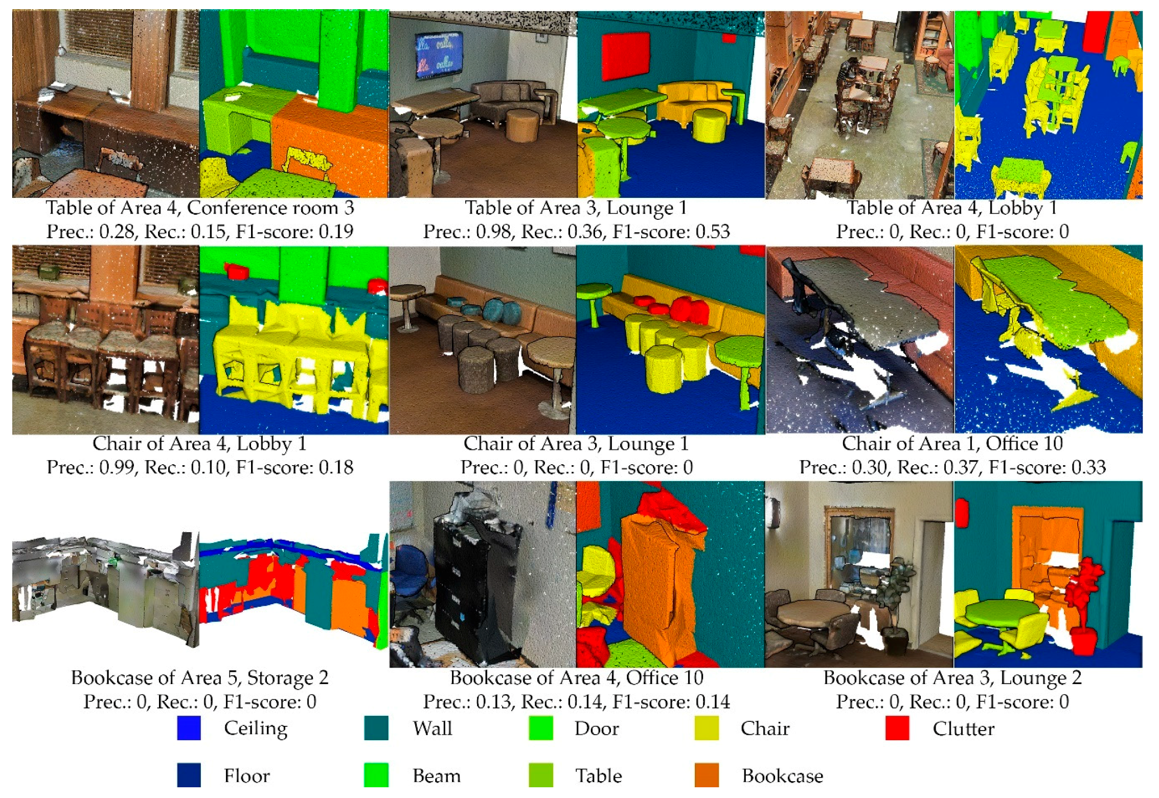
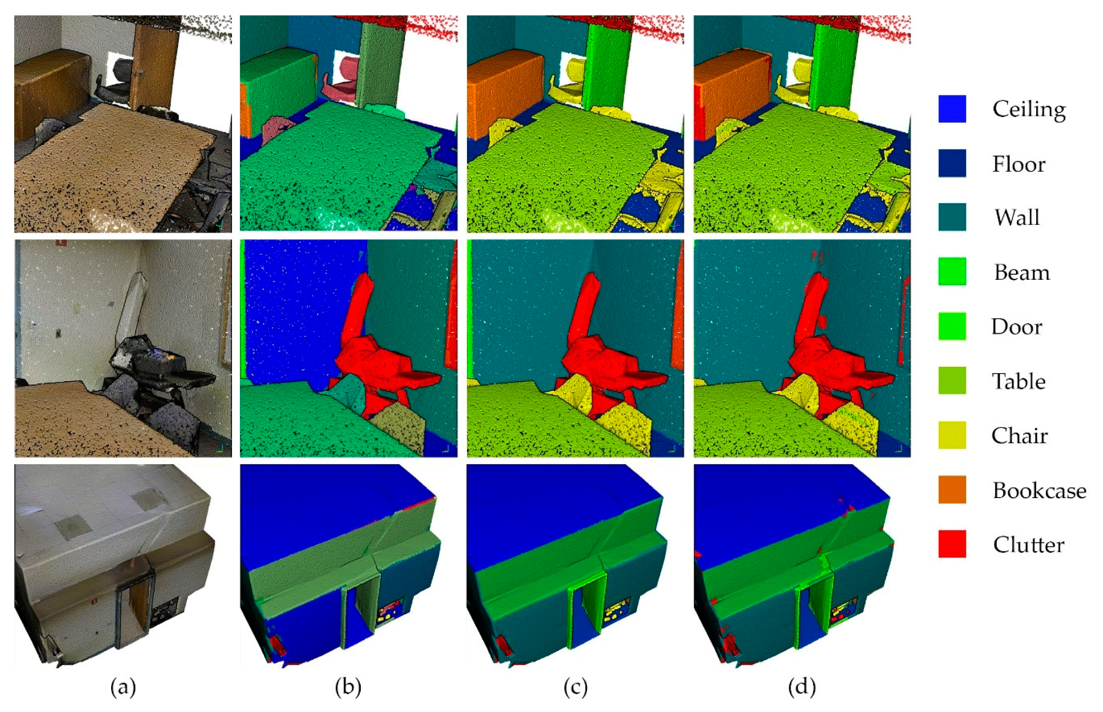
5.2. Quantitative and Qualitative Assessments

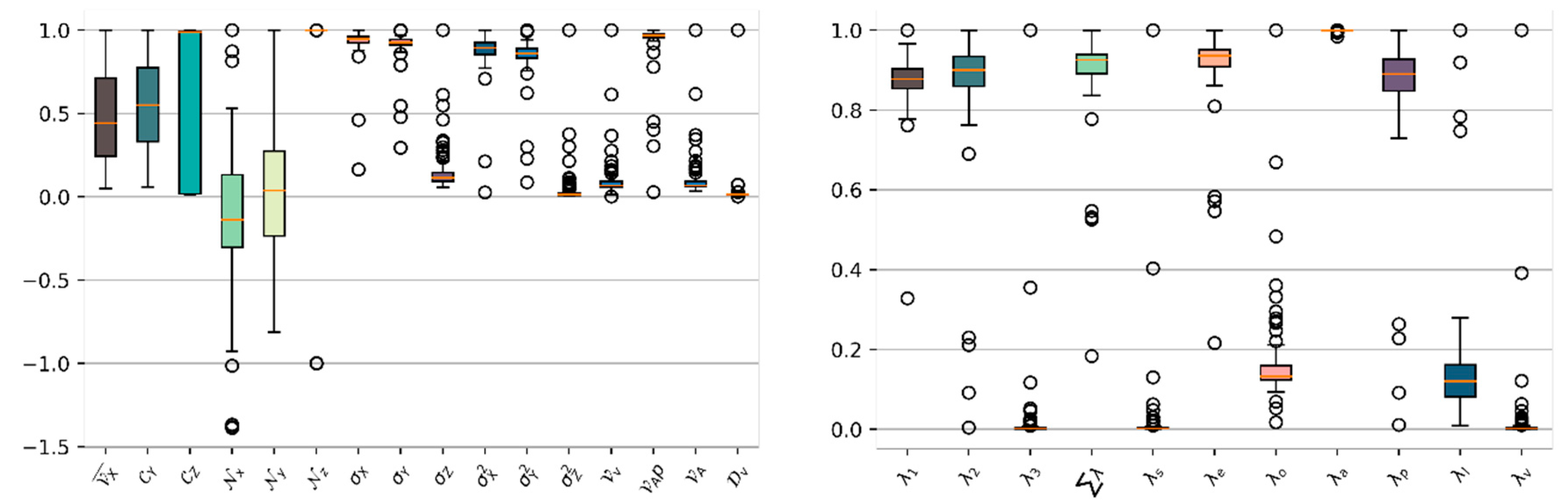
5.2.1. Feature Influence

Our first experiment independently uses SF1 and combined with SF2 to highlight performances and influence consequences on a representative sample from the S3DIS dataset. Table 6 lists the results regarding timings, number of CEL, elements (PE, SE, TE, RE) extracted and global metrics.
We note that SF1SF2 takes 30% longer, but permits obtaining 12 IoU points overall for Area-1, as well as 17 overall accuracy points and 12 F1-score points. For some rooms where the connectivity predicates are predominant, we can obtain more than a 30 IoU point increase. It is also very important to limit over-segmentation problematics while being versatile enough, depending on the different application needs. Thus, if we look at both the room and area 1 S3DIS samples, we note that the global number of CEL drops significantly, which permits classifier to reach a more representative detection (e.g., Table 7 gives an SF1SF2 instance detection comparison to ground truth).
We then applied our specific knowledge-based classification approach over both SF1 alone and SF1SF2.
Table 8 shows the metrics per class over the Area 1.
If we look at the IoU scores, combining SF1 and SF2 permits obtaining between +6 and +26 points (+13 points in average) when compared to SF1 alone, which is a notable increase of performances. The highest growth is achieved for the ‘chair’ class, and the lowest for the ‘door’ class. The 3D connectivity information given by SF2 through {PE, RE} isolation and clustering mostly explains the ‘chair’ detection rate increase, which permits overcoming SF1 matching limitations due to large varying signatures within voxels. Concerning doors, the low increase is explained by its low SF2 connectivity information as within the S3DIS dataset, door elements do not show any clear ‘cuts’ with wall elements, and therefore are not clearly identified within RE. This can be solved by accounting for colour information to better segment the point cloud, or by using the spatial context and empty voxels within the wall segments. Additionally, the high recall score for bookcase shows that the combination permits better accounting for the right number of bookcase elements. Overall, while we notice a slight precision score decrease for planar-based classes (ceiling, floor, wall), the recall rates largely increase between SF1 and SF1SF2. This highlights the ability of our classifier to better identify all of the positive samples. This is translated in F1-scores, which are superior for all classes up to +37 points.
Subsequently, we studied the impact of influential factors over the results and performance of the algorithm (experiments were run 50 times each to validate the time output), as shown in Figure 15.
We observe that our different metrics rise in a similar manner, with a greater score increase from octree level 4 to 5 (38 IoU points), and then not a distinctive increase. On the other end, we see an increase in the processing time from octree level 5 to 6, and a great increase from octree 6 to 7. This orients our choice towards a base process at octree level 5, sacrificing some score points for an adequate performance.

5.2.2. Full S3DIS Benchmark

We see that combining both SF1 and SF2 outperform a sole independent use of SF1 feature sets. Therefore, SF1SF2 method is compared against the state-of-the-art methodologies. We related our knowledge-based procedure to the best-performing supervised architectures due to the rise of deep learning approaches.
We first tested our semantic segmentation approach on the most complex area, Area 5, which holds a wide variety of rooms with varying size, architectural elements, and problematic cases. This is our worst-case scenario area. It holds different complex cases that the knowledge-based classification approach struggles to handle, and the results can be found in Appendix A. Concerning the performances and calculation times for Area-5 (68 rooms), our approaches finish in 59 min (3538.5 s) on average (10 test-run), whereas the well-performing SPG approach [49] allows for the classification of the Area (78 649 682 points) in 128.15 min (7689 s). Thus, while the results have a large improving margin for non-planar elements, the approach (without parallelization and low optimization) is very efficient. We provide more details in Section 5.3.
Subsequently, we execute our approach on the full S3DIS dataset, including varying problematic cases of which non-planar ceiling, stairs, heavy noise, heavy occlusion, false-labelled data, duplicate points, clutter, and non-planar walls comprise (see Appendix B for examples). This is a very good dataset for obtaining a robust indicator of how well a semantic segmentation approach performs and permitted to identify several failure cases, as illustrated in Figure 16.
We did not use any training data and our autonomous approach treats points by using only X, Y, Z coordinates. Again, we first use I o U ¯ metric to get an idea of the worst-case performances achieved by our classifier based on established Connected Elements summarized in Table 9.
We note that our approach proposes I o U ¯ scores of 85.4, 92.4 and 65.2 respectively for the ceiling, floor and wall classes. It is within a 3% to 15% range of achieved scores by every state-of-the-art method. This gives enough range for further improvements as discussed in Section 6. The ‘table’ elements present meagre performances explained by looking at Table 11 (high precision, low recall). Concerning bookcases our approach achieves poorly, partly due to the limitations of the knowledge-based approach. Indeed, the definition of a bookcase in Section 3.4 is not very flexible and doesn’t allows a search for hybrid structures where clutter on top of a bookcase hides planar patches thus classifying a bookcase as clutter and impacting I o U ¯ score of both classes. Yet, the ground-truth dataset presents a very high variability and discussable labelling as illustrated in Figure 16. The lowest score achieved concerns doors as identified previously. These elements are often misclassified as clutter, due to their SF1 signature and low SF2 characterization. Overall, our classification approach is comparable to the best deep learning approaches, and the very low computational demand as well as promising improvement flexibility due to the nature of Connected Elements will be further discussed in Section 6. Indeed, while the score is in general lower than the best performing deep-learning approaches, this is mainly due to the classification approach.
It is interesting to note that the deep learning architecture in Table 9 make use of colour information, whereas ours solely considers X, Y, Z attributes. A small benchmark is executed to account for this and provided in Table 10.
We see that we outperform PointNet when using only X, Y, Z data for ceiling, floor, and wall classes. To better understand where our classifier presents shortcomings, we studied F1-scores per Area and per class to obtain insights on problematic cases and possible guidelines for future works. The analysis can be found in Appendix C.
To summarize SF1SF2 performances, we present in Table 11 and the associated confusion matrix (Figure 17) per class scores over the full S3DIS dataset.
We note that we obtain in average a precision score of 0.75, a recall score of 0.72 thus a F1-score of 0.72. These are relatively good metrics considering the complexity of the test dataset, and the naïve classification approach. The largest improvement margin is linked to the ‘door’ and ‘bookcase’ classes as identified earlier and confirmed in Table 11. While for horizontal planar-dominant classes being ceiling and floor, the F1-scores of 0.92 and 0.96 give little place for improvement. It orients future work toward problematic cases handling (presented in Appendix B), and irregular structures targeting. The wall class detection scores of 0.79 gives a notable place for improvements, aiming both at a more precise and coherent classification approach. While table and chair precision are relatively good, their recall rate orients future work to better account for the full number of positive samples ignored with the present classification iteration. Looking at the normalized confusion matrix (denominator: 695 878 620 points in S3DIS), a large proportion of false positives are given to the clutter concerning all classes, which also demands a better precision in the recognition approach.
While the above metrics were compared against best-performing deep learning approaches, Table 12 permits to get a precise idea about how good the classifier achieves against the well-performing unsupervised baseline accessible in [16].
The used feature sets SF1/SF2 largely outperforms the baseline for the ceiling, floor, wall, table, and chair classes, permitting satisfying results, as illustrated in Figure 18.
However, we identified issues with the class ‘bookcase’ and ‘door’ where our approach performs poorly when compared to both the baseline with all features and without the colour. While the initial lack of SF2-related connectivity information mostly explains the door performance is mostly explained, as stated previously, the latter (bookcase) is partially linked to the variability under which it is found in the dataset and our too specialized classifier (indeed, we mostly consider ground-related bookcases which complicates the correct detection of wall-attached open bookcases). We thus noticed that several points were tagged as bookcase, whereas they are specifically desks or clutter (e.g., Figure 16).

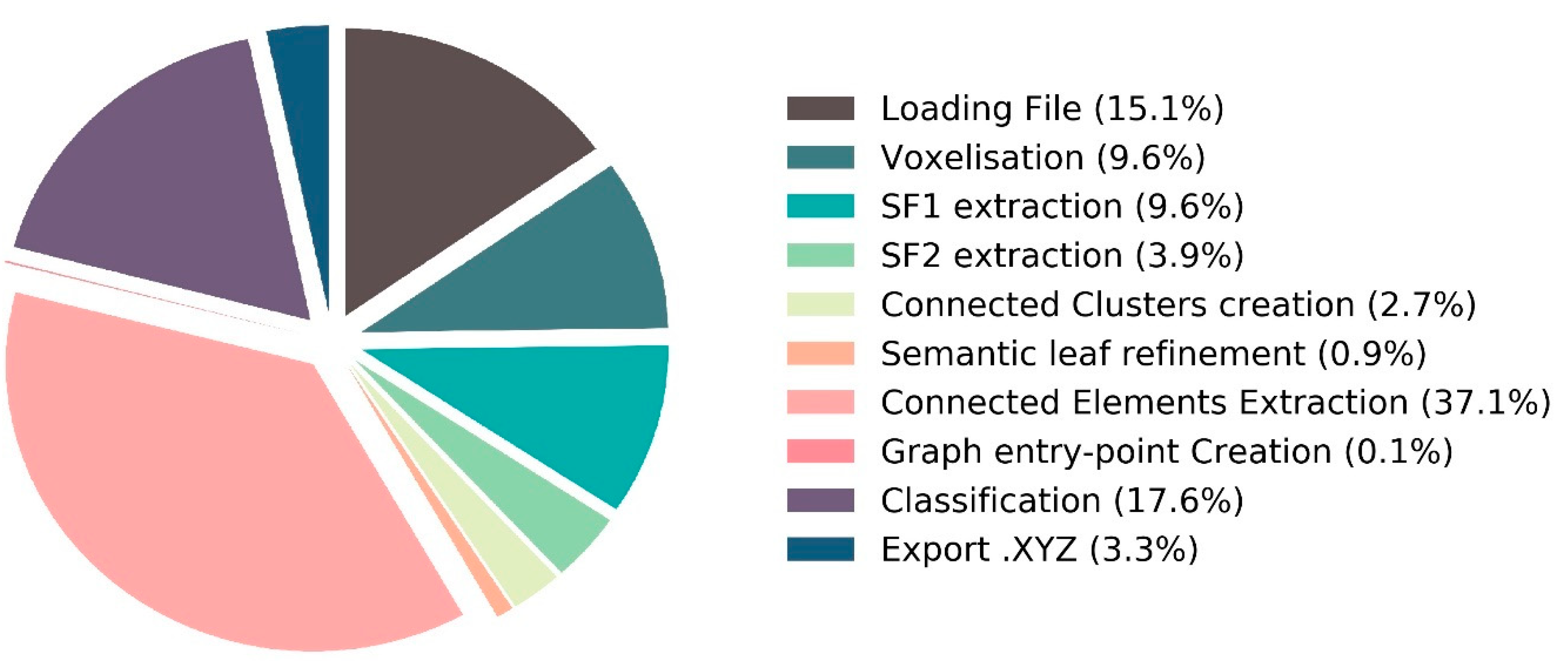
5.3. Implementation and Performances Details

The full autonomous parsing module was developed in Python 3.6. A limited number of libraries were used in order to easily replicate the developing environment, and thus the experiments and results. As such several functions were developed and will be accessible as open source for further research. All of the experiments were performed on a five years old laptop with a CPU Intel Core i7-4702HQ CPU @ 2.20Ghz, 16 Gb of RAM, and an Intel HD Graphics 4600. As currently standing (no optimization and no parallel processing), the approach is quite efficient and it permits processing, on average, 1.5 million points per minute. This allows offline computing to include in server-side infrastructures. Our approach is 54% faster if we compare its performance to a state-of-the-art approach, like [49] (2018), it does not necessitate any GPU, and it does not need any (important) training data.
By looking at the relative temporal performances (Figure 19), we note that the first computational hurdle is the creation of Connected Elements. This is mainly explained by the amount of handled points without any parallel computing, which can majorly reduce the needed time. Subsequently, it is followed by the classification approach, but, as our main goal was to provide a strong 3D structural connectivity structure for a Smart Point Cloud parsing module, we did not target the classification performances. Loading/Export times can be reduced if the input files are in the last format. The voxelisation approach and following steps until the semantic leaf extraction can also be parallelized for better performances. In the current version, 1.5 million points per minute are processed, on average, while using the above configuration without any GPU acceleration. It uses around 20% of the CPU and 900 Mb of RAM under full load. As it stands, it is therefore deployable on low-cost server-side infrastructures while giving the possibility of processing 90 million points per hour on average.

6. Discussion

From the detailed analysis provided in Section 5, we first summarize the identified strengths in the Section 6.1 and we then propose five main research directions for future work addressing the limitations in Section 6.2.

6.1. Strengths

First, the presented method is easy to implement. It is independent from any high-end GPUs, and mainly leverages the processor and the Random-Access Memory in its current state (around 1 Gb). This is crucial for a large number of companies that do not possess high-end servers, but rather web-oriented (no GPU, low RAM, and intel Core processors). As such, it is easily deployable on a client-server infrastructure, without the need to upgrade the server-side for offline computations.
Secondly, the approach is majorly unsupervised, which gives a great edge over (supervised) the machine learning approaches. Indeed, there is currently no need for a huge amount of training data, which thus avoids any time-consuming process of creating (and gathering) labelled datasets. This is particularly beneficial if one wants to create such a labelled dataset, as the provided methodology would speed-up the process by recognizing the main “host” elements of infrastructures, mainly leaving moveable elements supervision.
Third, on top of such a scenario, the approach provides acceptable results for various applications that mainly necessitate the determination of structural elements. As such, it can be used for extracting the surface of ceilings, walls, or floors if one wants to make digital quotations; it can provide a basis for extracting semantic spaces (sub-spaces) organized regarding their function; it can be used to provide a basis for floor plans, cut, section creation or visualization purposes [64,65].
Fourth, the provided implementation delivers adequate performances regarding the time that is needed for obtaining results. As it stands, without deep optimizations, it permits offline automatic segmentation and classification, and the data structure provides a parallel-computing support.
Fifth, there is a low input requirement that only necessitate unstructured X, Y, Z datasets, contrary to benchmarked Deep Learning approaches that leverage colour information and provide a complete directed graph of the relations within CELs or classified objects. This information permits reasoning services to use the semantic connectivity information between objects and subspaces for advanced queries using both spatial and semantic attributes.
Finally, the unsupervised segmentation and rule-based classification is easily extensible by improving the feature determination, enhancing the performances, or providing a better and more flexible classifier. For example, one can differentiate clutter based on connectivity and proximities to further enhance the classification (e.g., clutter on top of a table may be a computer; clutter linked to the ceiling and in the middle of the room is a light source…). Some of these potentials are addressed as research tracks for future works, as presented in the following Section 6.2.

6.2. Limitations and Research Directions

First, we note that the new relational features are very useful in the task of semantic segmentation. Plugged to a basic knowledge-based graph, it permits good planar-elements detection, such as floor, ceiling, and wall. At this point, it is quite useful for the creation of Connected Elements as all of the remaining points mainly cover remaining “floating” elements, which can then be further defined through classification routines. This is a very interesting perspective for higher end specialization per application, where the remaining elements are then looped for accurate refinement depending on the level of specialization needed, as expressed in [52]. Future work will also further study learning-based feature extraction, such as the ones presented in [66,67], proposing a design of the shape context descriptor with spatially inhomogeneous cells. The parsing methodology can also be extended through other domain ontologies, such as the CIDOC-CRM, as presented in [68], which highlight the flexibility to different domains.
Secondly, the creation of links between CEL is a novelty that provides interesting perspectives concerning reasoning possibilities that play on relationships between elements. Indeed, the extracted graph is fully compatible with the semantic web and it can be used as a base for reasoning services, and provide counting possibilities, such as digital inventories [68] and semantic modelling [59]. Additionally, the decomposition in primary, secondary, transition, and rest elements is very useful in such contexts, as one can specialize or aggregate elements depending on the intended use and application [50]. Indeed, the approach permits obtaining a precise representation of the underlying groups of point contained within Connected Elements and homogenized in Semantic Patches.
Third, the extended benchmark proved that untrained schemes could reach a comparable recognition rate to the best-performing deep learning architectures. Particularly, detecting the main structural elements permits achieving a good first semantic representation of space, opening the approach to several applications. However, the scores for ‘floating’ CEL (moveable elements) is poor in its current version. Shortcomings are linked to the naïve knowledge-based classifier, which lacks flexibility/generalization in its conception and gives place for major improvements in future works. Specifically, it will undergo an ontology formalization to provide a higher characterization and moving thresholds to better adapt the variability in which elements are found in the dataset.
Fourth, some artefacts and performances hurt the approach due to the empirical octree-based voxelization determination and enactment, but, as it stands, it provides a stable structure that is robust to aliasing and the blocking effect at the borders. Further works in the direction of efficient parallel computing will permit an increase in time performances and deeper depth tree selection (thus better characterization). Additionally, the octree definition will be looked at for variable octree depth, depending on pre-define sensor-related voxel leaf size. Other possibilities include using a local voxelated structure, such as that proposed in [54] to encode the local shape structure into bit string by point spatial locations without computing complex geometric attributes. On the implementation side, while the dependency to voxelization is limited due to the octree structure to allow a constant point density per voxel, on average, it will be further studied to avoid exponential time explosion when changing the deepness level. As such, the structure is already ready for parallel computing and it will be studied in future works.
Finally, while our dedicated approach was tested on the S3DIS dataset, it can easily be adapted to other point clouds that provide an additional research direction. The approach will be tested against indoor and outdoor point clouds from different sensors and the classification could be adapted to account for various well-established classes. As such, a large effort is currently undergoing to create accurate labelled datasets for AEC and outdoor 3D mapping applications, to be shared as open-data.
Our focus is driven by a general global/local contextualization of digital 3D environments, where we aim at providing a flexible infrastructure that should be able to scale up to different generalization levels. As such, the proposed unsupervised segmentation approach in Connected Elements and Semantic patches acts as a standard module within the Smart Point Cloud Infrastructure and permit obtaining a full autonomous workflow for the constitution of semantically rich point clouds [2].

7. Conclusions

In this article, a point cloud parsing module for a Smart Point Cloud Infrastructure was presented. It provides a semantic segmentation framework that groups points in a voxel-based space, where each voxel is studied by analytic featuring and similarity analysis to define the semantic clusters that retain highly representative SF1 and SF2 signatures. This process is conducted regarding an initial connected component from multi-composed graph representations after automatically detecting different planar-dominant elements leveraging their prevalence in man-made environments. A classification approach to automatically detect main classes in the S3DIS dataset and obtain a measure of performance against best-performing deep learning approaches is provided. While the method is well performing for the floor, ceiling, and wall classes, extended research is needed if one wants to use the classification as a robust approach for moveable elements detection.

Author Contributions

Conceptualization, Florent Poux; Methodology, Florent Poux; Software, Florent Poux; Validation, Florent Poux; Formal Analysis, Florent Poux; Investigation, Florent Poux; Resources, Florent Poux; Data Curation, Florent Poux; Writing-Original Draft Preparation, Florent Poux; Writing-Review & Editing, Florent Poux & Roland Billen; Visualization, Florent Poux; Supervision, Florent Poux & Roland Billen.

Funding

This research received no external funding.

Acknowledgments

We would like to thank the research community in general for their interest in point cloud semantic segmentation, and to permit a rapid evolution of the technology.

Conflicts of Interest

The authors declare no conflict of interest.

Appendix A

We decided to hold I o U ¯ metrics to get an idea of the worst possible scores and compare them with the three methods listed in Table A1:
Table A1. Intersection-over-Union on Area 5 of our methodology compared to PointNet [25], SegCloud [48] and SuperPoint Graphs (SPG [49]).
IoU for Area-5CeilingFloorWallBeamDoorTableChairBookcaseClutter
01236781012
PointNet [25]88.897.3369.80.0510.7658.9352.6140.2833.22
SegCloud [48]90.0696.0569.86023.1270.475.8958.4241.6
SPG [49]91.4997.8975.89052.2977.486.3565.4950.67
Ours85.7892.9171.3207.5431.1529.0223.4821.91
We see that scores obtained for the floor and the ceilings are comparable to the ones obtained by the three deep learning approaches. However, the wall detection ratio outperforms both PointNet and SegCloud, but SPG are still showing better performances. This is explained by the high level of noise and irregular structure. The beam presents a null score (as benchmarked methods) due to the very little number of points and specificity of the 3 beams in the ground truth dataset labelled containing 22 424 points.
Ijgi 08 00213 i004

Appendix B

Ijgi 08 00213 i005

Appendix C

We provide the summary of our analysis conducted per area in Table A2.
Table A2. Summary of the 6 areas using our semantic segmentation approach.
F1-scoreCeilingFloorWallBeamDoorTableChairBookcaseClutter
01236781012
Area-10.970.960.800.660.240.480.480.260.47
Area-20.850.940.700.150.220.110.120.260.32
Area-30.980.980.780.610.210.410.610.380.50
Area-40.900.970.780.000.120.250.400.240.35
Area-50.920.960.830.000.140.480.450.380.36
Area-60.950.970.780.580.240.540.530.280.43
We note that Area-2 is responsible for a drop of performance in ceiling and floor detection, as well as Area-4, which is explained by the very irregular structures of the ceiling and the presence of multilevel stairs. Wall detection is constant among areas whereas beams are very irregular and explain the drop of performances in non-weighted. The classes in Areas 2, 4 and 5 are very specific and in a very low number of occurrences (see Table A2). Table and chair detection rates are very constant and give place for future improvements. Bookcase and clutter also show very similar detection rates per area and demand a global classification optimization for higher performances.
As seen above, ‘table’ presents an unsatisfying detection rate. This is due to the very low recall score, as our classifier only tagged points which were surely a table.
Ijgi 08 00213 i006aIjgi 08 00213 i006b

References

  1. Koffka, K. Principles of Gestalt Psychology; Routledge: Abingdon-on-Thames, UK, 2013. [Google Scholar]
  2. Poux, F.; Billen, R. A Smart Point Cloud Infrastructure for intelligent environments. In Laser Scanning: An Emerging Technology in Structural Engineering; Lindenbergh, R., Belen, R., Eds.; ISPRS Book Series; Taylor & Francis Group/CRC Press: Bocaton, FL, USA, 2019; in press. [Google Scholar]
  3. Yang, B.; Luo, W.; Urtasun, R. PIXOR: Real-time 3D Object Detection from Point Clouds. In Proceedings of the Conference on Computer Vision and Pattern Recognition (CVPR), Salt Lake City, UT, USA, 18–22 June 2018; pp. 7652–7660. [Google Scholar]
  4. Rostami, R.; Bashiri, F.S.; Rostami, B.; Yu, Z. A Survey on Data-Driven 3D Shape Descriptors. Comput. Graph. Forum 2018, 38, 1–38. [Google Scholar] [CrossRef]
  5. Su, H.; Jampani, V.; Sun, D.; Maji, S.; Kalogerakis, E.; Yang, M.H.; Kautz, J. SPLATNet: Sparse Lattice Networks for Point Cloud Processing. In Proceedings of the Conference on Computer Vision and Pattern Recognition (CVPR), Salt Lake City, UT, USA, 18–22 June 2018; pp. 2530–2539. [Google Scholar]
  6. Boulch, A.; Le Saux, B.; Audebert, N. Unstructured point cloud semantic labeling using deep segmentation networks. In Proceedings of the Eurographics Workshop on 3D Object Retrieval; EUROGRAPHICS: Lyon, France, 2017. [Google Scholar]
  7. Liao, Y.; Donné, S.; Geiger, A. Deep Marching Cubes: Learning Explicit Surface Representations. In Proceedings of the Conference on Computer Vision and Pattern Recognition (CVPR), Salt Lake City, UT, USA, 18–22 June 2018; pp. 2916–2925. [Google Scholar]
  8. Thomas, H.; Goulette, F.; Deschaud, J.E.; Marcotegui, B.; Gall, Y. Le Semantic classification of 3d point clouds with multiscale spherical neighborhoods. In Proceedings of the International Conference on 3D Vision (3DV), Verona, Italy, 5–8 September 2018; pp. 390–398. [Google Scholar]
  9. Jiang, M.; Wu, Y.; Lu, C. PointSIFT: A SIFT-like Network Module for 3D Point Cloud Semantic Segmentation. Comput. Vis. Pattern Recognit. 2018, arXiv:1807.00652. [Google Scholar]
  10. Nguyen, C.; Starek, M.J.; Tissot, P.; Gibeaut, J. Unsupervised clustering method for complexity reduction of terrestrial lidar data in marshes. Remote Sens. 2018, 10, 133. [Google Scholar] [CrossRef]
  11. Behl, A.; Paschalidou, D.; Donné, S.; Geiger, A. PointFlowNet: Learning Representations for 3D Scene Flow Estimation from Point Clouds. Comput. Vis. Pattern Recognit. 2018, arXiv:1806.02170. [Google Scholar]
  12. Engelmann, F.; Kontogianni, T.; Schult, J.; Leibe, B. Know What Your Neighbors Do: 3D Semantic Segmentation of Point Clouds. In Proceedings of the European Conference on Computer Vision (ECCV), Munich, Germany, 8–14 September 2018. [Google Scholar]
  13. Li, J.; Chen, B.M.; Lee, G.H. SO-Net: Self-Organizing Network for Point Cloud Analysis. In Proceedings of the Conference on Computer Vision and Pattern Recognition (CVPR), Salt Lake City, UT, USA, 18–22 June 2018. [Google Scholar]
  14. Guerrero, P.; Kleiman, Y.; Ovsjanikov, M.; Mitra, N.J. PCPNet learning local shape properties from raw point clouds. Comput. Graph. Forum 2018, 37, 75–85. [Google Scholar] [CrossRef]
  15. Boulch, A.; Guerry, J.; Le Saux, B.; Audebert, N. SnapNet: 3D point cloud semantic labeling with 2D deep segmentation networks. Comput. Graph. 2018, 71, 189–198. [Google Scholar] [CrossRef]
  16. Armeni, I.; Sener, O.; Zamir, A.R.; Jiang, H.; Brilakis, I.; Fischer, M.; Savarese, S. 3D Semantic Parsing of Large-Scale Indoor Spaces. In Proceedings of the Conference on Computer Vision and Pattern Recognition (CVPR), Las Vegas, NV, USA, 26 June–1 July 2016; pp. 1534–1543. [Google Scholar]
  17. Ni, H.; Lin, X.; Zhang, J.; Ni, H.; Lin, X.; Zhang, J. Classification of ALS Point Cloud with Improved Point Cloud Segmentation and Random Forests. Remote Sens. 2017, 9, 288. [Google Scholar] [CrossRef]
  18. Ghorpade, V.K.; Checchin, P.; Malaterre, L.; Trassoudaine, L. 3D shape representation with spatial probabilistic distribution of intrinsic shape keypoints. EURASIP J. Adv. Signal Process. 2017, 2017, 52. [Google Scholar] [CrossRef]
  19. Bueno, M.; Martínez-Śanchez, J.; Gonźalez-Jorge, H.; Lorenzo, H. Detection of geometric keypoints and its application to point cloud coarse registration. In Proceedings of the International Archives of the Photogrammetry, Remote Sensing and Spatial Information Sciences - ISPRS Archives; ISPRS: Prague, Czech Republic, 2016; Volume 41, pp. 187–194. [Google Scholar]
  20. Vetrivel, A.; Gerke, M.; Kerle, N.; Nex, F.; Vosselman, G. Disaster damage detection through synergistic use of deep learning and 3D point cloud features derived from very high resolution oblique aerial images, and multiple-kernel-learning. ISPRS J. Photogramm. Remote Sens. 2018, 140, 45–59. [Google Scholar] [CrossRef]
  21. Poux, F.; Neuville, R.; Hallot, P.; Van Wersch, L.; Jancsó, A.L.; Billen, R. Digital investigations of an archaeological smart point cloud: A real time web-based platform to manage the visualisation of semantical queries. Int. Arch. Photogramm. Remote Sens. Spat. Inf. Sci. - ISPRS Arch. 2017, XLII-5/W1, 581–588. [Google Scholar] [CrossRef]
  22. Blomley, R.; Weinmann, M.; Leitloff, J.; Jutzi, B. Shape distribution features for point cloud analysis—A geometric histogram approach on multiple scales. In Proceedings of the ISPRS Annals of the Photogrammetry, Remote Sensing and Spatial Information Sciences; ISPRS: Zurich, Switzerland, 2014; Volume 2, pp. 9–16. [Google Scholar]
  23. Feng, C.C.; Guo, Z. Automating parameter learning for classifying terrestrial LiDAR point cloud using 2D land cover maps. Remote Sens. 2018, 10, 1192. [Google Scholar] [CrossRef]
  24. Shen, Y.; Feng, C.; Yang, Y.; Tian, D. Mining Point Cloud Local Structures by Kernel Correlation and Graph Pooling. In Proceedings of the Conference on Computer Vision and Pattern Recognition (CVPR), Salt Lake City, UT, USA, 18–22 June 2018; pp. 4548–4557. [Google Scholar]
  25. Qi, C.R.; Su, H.; Mo, K.; Guibas, L.J. PointNet: Deep learning on point sets for 3D classification and segmentation. In Proceedings of the Conference on Computer Vision and Pattern Recognition (CVPR), Honolulu, HI, USA, 21 June–26 July 2017; pp. 77–85. [Google Scholar]
  26. Nurunnabi, A.; Belton, D.; West, G. Robust Segmentation for Large Volumes of Laser Scanning Three-Dimensional Point Cloud Data. IEEE Trans. Geosci. Remote Sens. 2016, 54, 4790–4805. [Google Scholar] [CrossRef]
  27. Lawin, F.J.; Danelljan, M.; Tosteberg, P.; Bhat, G.; Khan, F.S.; Felsberg, M. Deep projective 3D semantic segmentation. In Proceedings of the Computer Analysis of Images and Patterns (CAIP), Ystad, Sweden, 22–24 August 2017; pp. 95–107. [Google Scholar]
  28. Mahmoudabadi, H.; Shoaf, T.; Olsen, M.J. Superpixel clustering and planar fit segmentation of 3D LIDAR point clouds. In Proceedings of the 4th International Conference on Computing for Geospatial Research and Application, (COM.Geo), New York, NY, USA, 22–24 July 2013; pp. 1–7. [Google Scholar]
  29. Ioannou, Y.; Taati, B.; Harrap, R.; Greenspan, M. Difference of normals as a multi-scale operator in unorganized point clouds. In Proceedings of the 3D Imaging, Modeling, Processing, Visualization and Transmission (3DIMPVT); IEEE: Zurich, Switzerland, 2012; pp. 501–508. [Google Scholar]
  30. Vosselman, G.; Gorte, B.G.H.; Sithole, G.; Rabbani, T. Recognising structure in laser scanner point clouds. In Proceedings of the International Archives of the Photogrammetry, Remote Sensing and Spatial Information Sciences-ISPRS Archives; ISPRS: Freiburg, Germany, 2003; Volume 46, pp. 33–38. [Google Scholar]
  31. Song, T.; Xi, F.; Guo, S.; Ming, Z.; Lin, Y. A comparison study of algorithms for surface normal determination based on point cloud data. Precis. Eng. 2015, 39, 47–55. [Google Scholar] [CrossRef]
  32. Weber, C.; Hahmann, S.; Hagen, H. Sharp feature detection in point clouds. In Proceedings of the International Conference on Shape Modeling and Applications; IEEE: Washington, DC, USA, 2010; pp. 175–186. [Google Scholar]
  33. Ni, H.; Lin, X.; Ning, X.; Zhang, J. Edge Detection and Feature Line Tracing in 3D-Point Clouds by Analyzing Geometric Properties of Neighborhoods. Remote Sens. 2016, 8, 710. [Google Scholar] [CrossRef]
  34. Schnabel, R.; Wahl, R.; Klein, R. Efficient RANSAC for Point Cloud Shape Detection. Comput. Graph. Forum 2007, 26, 214–226. [Google Scholar] [CrossRef]
  35. Fischler, M.A.; Bolles, R.C. Random sample consensus: A paradigm for model fitting with applications to image analysis and automated cartography. Commun. ACM 1981, 24, 381–395. [Google Scholar] [CrossRef]
  36. Hackel, T.; Wegner, J.D.; Schindler, K. Joint classification and contour extraction of large 3D point clouds. ISPRS J. Photogramm. Remote Sens. 2017, 130, 231–245. [Google Scholar] [CrossRef]
  37. Son, H.; Kim, C. Semantic as-built 3D modeling of structural elements of buildings based on local concavity and convexity. Adv. Eng. Inf. 2017, 34, 114–124. [Google Scholar] [CrossRef]
  38. Wang, J.; Lindenbergh, R.; Menenti, M. SigVox—A 3D feature matching algorithm for automatic street object recognition in mobile laser scanning point clouds. ISPRS J. Photogramm. Remote Sens. 2017, 128, 111–129. [Google Scholar] [CrossRef]
  39. Liu, Y.-S.; Ramani, K. Robust principal axes determination for point-based shapes using least median of squares. Comput. Aided Des. 2009, 41, 293–305. [Google Scholar] [CrossRef]
  40. Xu, Y.; Tuttas, S.; Hoegner, L.; Stilla, U. Voxel-based segmentation of 3D point clouds from construction sites using a probabilistic connectivity model. Pattern Recognit. Lett. 2018, 102. [Google Scholar] [CrossRef]
  41. Xu, Y.; Hoegner, L.; Tuttas, S.; Stilla, U. Voxel- and Graph-Based Point Cloud Segmentation of 3D Scenes Using Perceptual Grouping Laws. In Proceedings of the ISPRS Annals of the Photogrammetry, Remote Sensing and Spatial Information Sciences; ISPRS: Hannover, Germany, 2017; Volume 4, pp. 43–50. [Google Scholar]
  42. Zhu, Q.; Li, Y.; Hu, H.; Wu, B. Robust point cloud classification based on multi-level semantic relationships for urban scenes. ISPRS J. Photogramm. Remote Sens. 2017, 129, 86–102. [Google Scholar] [CrossRef]
  43. Wang, Y.; Cheng, L.; Chen, Y.; Wu, Y.; Li, M. Building point detection from vehicle-borne LiDAR data based on voxel group and horizontal hollow analysis. Remote Sens. 2016, 8, 419. [Google Scholar] [CrossRef]
  44. Ben-Shabat, Y.; Avraham, T.; Lindenbaum, M.; Fischer, A. Graph based over-segmentation methods for 3D point clouds. Comput. Vis. Image Underst. 2018, 174, 12–23. [Google Scholar] [CrossRef]
  45. Ben-Shabat, Y.; Lindenbaum, M.; Fischer, A. 3D Point Cloud Classification and Segmentation Using 3D Modified Fisher Vector Representation for Convolutional Neural Networks. Available online: http://arxiv.org/abs/1711.08241 (accessed on 31 October 2018).
  46. Rusu, R.B.; Blodow, N.; Beetz, M. Fast Point Feature Histograms (FPFH) for 3D registration. In Proceedings of the International Conference on Robotics and Automation (ICRA); IEEE: Kobe, Japan, 2009; pp. 3212–3217. [Google Scholar]
  47. Qi, C.R.; Yi, L.; Su, H.; Guibas, L.J. PointNet++: Deep Hierarchical Feature Learning on Point Sets in a Metric Space. In Proceedings of the Conference on Neural Information Processing Systems (NIPS), Long Beach, CA, USA, 24 January 2019. [Google Scholar]
  48. Tchapmi, L.P.; Choy, C.B.; Armeni, I.; Gwak, J.; Savarese, S. SEGCloud: Semantic Segmentation of 3D Point Clouds. In Proceedings of the International Conference on 3D Vision (3DV), Qingdao, China, 10–12 October 2017. [Google Scholar]
  49. Landrieu, L.; Simonovsky, M. Large-Scale Point Cloud Semantic Segmentation with Superpoint Graphs. In Proceedings of the Conference on Computer Vision and Pattern Recognition (CVPR), Salt Lake City, UT, USA, 18–22 June 2018; pp. 4558–4567. [Google Scholar]
  50. Poux, F.; Neuville, R.; Hallot, P.; Billen, R. MODEL FOR SEMANTICALLY RICH POINT CLOUD DATA. ISPRS Ann. Photogramm. Remote Sens. Spat. Inf. Sci. 2017, IV-4/W5, 107–115. [Google Scholar] [CrossRef]
  51. Engelmann, F.; Kontogianni, T.; Hermans, A.; Leibe, B. Exploring Spatial Context for 3D Semantic Segmentation of Point Clouds. In Proceedings of the International Conference on Computer Vision (ICCV); IEEE: Istanbul, Turkey, 2018; pp. 716–724. [Google Scholar]
  52. Poux, F.; Hallot, P.; Neuville, R.; Billen, R. SMART POINT CLOUD: DEFINITION AND REMAINING CHALLENGES. ISPRS Ann. Photogramm. Remote Sens. Spat. Inf. Sci. 2016, IV-2/W1, 119–127. [Google Scholar] [CrossRef]
  53. Truong-Hong, L.; Laefer, D.F.; Hinks, T.; Carr, H. Flying Voxel Method with Delaunay Triangulation Criterion for Façade/Feature Detection for Computation. J. Comput. Civ. Eng. 2012, 26, 691–707. [Google Scholar] [CrossRef]
  54. Quan, S.; Ma, J.; Hu, F.; Fang, B.; Ma, T. Local voxelized structure for 3D binary feature representation and robust registration of point clouds from low-cost sensors. Inf. Sci. (Ny). 2018, 444, 153–171. [Google Scholar] [CrossRef]
  55. Poux, F.; Neuville, R.; Hallot, P.; Billen, R. Point clouds as an efficient multiscale layered spatial representation. In Proceedings of the Eurographics Workshop on Urban Data Modelling and Visualisation; Vincent, T., Biljecki, F., Eds.; The Eurographics Association: Liège, Belgium, 2016. [Google Scholar]
  56. Nourian, P.; Gonçalves, R.; Zlatanova, S.; Ohori, K.A.; Vu Vo, A. Voxelization algorithms for geospatial applications: Computational methods for voxelating spatial datasets of 3D city models containing 3D surface, curve and point data models. MethodsX 2016, 3, 69–86. [Google Scholar] [CrossRef]
  57. Weinmann, M.; Jutzi, B.; Hinz, S.; Mallet, C. Semantic point cloud interpretation based on optimal neighborhoods, relevant features and efficient classifiers. ISPRS J. Photogramm. Remote Sens. 2015, 105, 286–304. [Google Scholar] [CrossRef]
  58. De Lathauwer, L.; De Moor, B.; Vandewalle, J. A Multilinear Singular Value Decomposition. SIAM J. Matrix Anal. Appl. 2003, 21, 1253–1278. [Google Scholar] [CrossRef]
  59. Poux, F.; Neuville, R.; Nys, G.-A.; Billen, R. 3D Point Cloud Semantic Modelling: Integrated Framework for Indoor Spaces and Furniture. Remote Sens. 2018, 10, 1412. [Google Scholar] [CrossRef]
  60. Clementini, E.; Di Felice, P. Approximate topological relations. Int. J. Approx. Reason. 1997, 16, 173–204. [Google Scholar] [CrossRef]
  61. He, L.; Ren, X.; Gao, Q.; Zhao, X.; Yao, B.; Chao, Y. The connected-component labeling problem: A review of state-of-the-art algorithms. Pattern Recognit. 2017, 70, 25–43. [Google Scholar] [CrossRef]
  62. Krijnen, T.; Beetz, J. An IFC schema extension and binary serialization format to efficiently integrate point cloud data into building models. Adv. Eng. Inform. 2017, 33, 473–490. [Google Scholar] [CrossRef]
  63. Lehtola, V.; Kaartinen, H.; Nüchter, A.; Kaijaluoto, R.; Kukko, A.; Litkey, P.; Honkavaara, E.; Rosnell, T.; Vaaja, M.; Virtanen, J.-P.; et al. Comparison of the Selected State-Of-The-Art 3D Indoor Scanning and Point Cloud Generation Methods. Remote Sens. 2017, 9, 796. [Google Scholar] [CrossRef]
  64. Neuville, R.; Pouliot, J.; Poux, F.; Billen, R. 3D Viewpoint Management and Navigation in Urban Planning: Application to the Exploratory Phase. Remote Sens. 2019, 11, 236. [Google Scholar] [CrossRef]
  65. Neuville, R.; Pouliot, J.; Poux, F.; de Rudder, L.; Billen, R. A Formalized 3D Geovisualization Illustrated to Selectivity Purpose of Virtual 3D City Model. ISPRS Int. J. Geo-Inf. 2018, 7, 194. [Google Scholar] [CrossRef]
  66. Belongie, S.; Malik, J.; Puzicha, J. Shape matching and object recognition using shape contexts. IEEE Trans. Pattern Anal. Mach. Intell. 2002, 24, 509–522. [Google Scholar] [CrossRef]
  67. Liu, S.; Xie, S.; Chen, Z.; Tu, Z. Attentional ShapeContextNet for Point Cloud Recognition. Conf. Comput. Vis. Pattern Recognit. 2018, 4606–4615. [Google Scholar]
  68. Poux, F.; Neuville, R.; Van Wersch, L.; Nys, G.-A.; Billen, R. 3D Point Clouds in Archaeology: Advances in Acquisition, Processing and Knowledge Integration Applied to Quasi-Planar Objects. Geosciences 2017, 7, 96. [Google Scholar] [CrossRef]
Figure 1. Voxel-based three-dimensional (3D) semantic segmentation. From left to right: Raw point cloud, feature engineering, Connected Elements extraction, Classified point cloud.
Ijgi 08 00213 g001
Figure 2. Visual patterns on points from left to right: Not grouped; Proximity criterion; Similarity criterion; Common cluster region; Linear criterion; Parallel criterion: Symmetry criterion.
Ijgi 08 00213 g002
Figure 3. Methodological workflow for the constitution of Connected Elements and knowledge-based classification. A point cloud goes through seven serialized steps (diamonds) to obtain a fully classified dataset (red square).
Ijgi 08 00213 g003
Figure 4. Point Cloud and its extracted voxel structure, where each octree level represents the grid voxels, each subdivided in subsequent eight voxel children.
Ijgi 08 00213 g004
Figure 5. Feature transfer between octree levels. We note that each non-empty node describes a voxel which can then permit a point-level access for example to compute feature sets (here, a planar voxel and a corresponding SF1 sample, and a transition voxel and its corresponding SF1 sample).
Ijgi 08 00213 g005
Figure 6. Box plot of primary elements feature variation.
Ijgi 08 00213 g006
Figure 7. Direct voxel-to-voxel topology in a 26-connectivity graph. Considered voxel V i is red, direct connections are either vertex.touch (grey), edge.touch (yellow), or face.touch (orange).
Ijgi 08 00213 g007
Figure 8. Relationship tagging in the voxel-space. (a) represent a mixed relationship M r , (b) a pure vertical relationship V r , and (c) a pure horizontal relationship H r .
Ijgi 08 00213 g008
Figure 9. S3DIS points within categorized voxels. (a) Full transition voxels, (b) vertical group of points, (c) horizontal group of points, and (d) mixed group of points.
Ijgi 08 00213 g009
Figure 10. Graph representation within a voxel sample of the point cloud.
Ijgi 08 00213 g010
Figure 11. Elements detection and categorization. A point cloud is search for Primary Elements (PE), the rest is searched for Secondary elements (SE). The remaining from this step is searched for transition elements (TE), leaving remaining elements (RE). TE permits extracting graphs through SF2 analysis with PE, SE, and RE.
Ijgi 08 00213 g011
Figure 12. Edges elements to be decomposed in TE and RE.
Ijgi 08 00213 g012
Figure 13. Different graphs generated on voxel categories. (a) Connected Elements (CEL) graph, (b) PE graph, (c) SE graph, (d) TE graph, and (e) RE graph.
Ijgi 08 00213 g013
Figure 14. (a) Raw point cloud; (b) {PE, SE, TE, RE} groups of voxels; (c) Connected Elements; and, (d) Classified point cloud.
Ijgi 08 00213 g014
Figure 15. Normalized score and processing time in function of the defined octree level.
Ijgi 08 00213 g015
Figure 16. Problematics cases which often include point cloud artefacts such as heavy noise, missing parts, irregular shape geometries, mislabelled data.
Ijgi 08 00213 g016
Figure 17. Normalized Confusion matrix of our semantic segmentation approach over the full S3DIS dataset.
Ijgi 08 00213 g017
Figure 18. Results of the semantic segmentation on a room sample. (a) RGB point cloud, (b) Connected Elements, (c) Ground Truth, and (d) Results of the semantic segmentation.
Ijgi 08 00213 g018
Figure 19. Relative temporal performances of our automatic semantic segmentation workflow.
Ijgi 08 00213 g019
Table 1. Eigen-based features part of the SF1 feature set.
Eigen-Based FeatureDescription
λ 1 , λ 2 , λ 3 Eigen values of V i , j , k where λ 1 > λ 2 > λ 3 Ijgi 08 00213 i001
v 1 ,   v 2 ,   v 3 Respective Eigen vectors of V i , j , k
v 3 Normal vector of V i , j , k
λ a Anisotropy of voxel V i , j , k
λ e Eigen entropy of voxel V i , j , k
λ l Linearity of voxel V i , j , k
λ o Omnivariance of voxel V i , j , k
λ p Planarity of voxel V i , j , k
λ s Sphericity of voxel V i , j , k
λ v Surface variation of voxel V i , j , k
Table 2. Geometrical features part of the SF1 feature set.
Geometrical FeatureDescription
V i x ¯ ,   V i y ¯ ,   V i z ¯ Mean value of points in V i , j , k respectively along e x , e y , e z Ijgi 08 00213 i002
σ i x 2 , σ i y 2 , σ i z 2 Variance of points in voxel V i , j , k
V A p Area of points in V i , j , k along n V ( v 3 )
V A Area of points in V i , j , k along e z
m Number of points in V i , j , k
V V Volume occupied by points in V i , j , k
D V point density within voxel V i , j , k
Table 3. Relational features of the SF2 feature set for three-dimensional (3D) structural connectivity.
Relational Feature Description
g 26 ( i ) Graph of voxel entity i and its neighbours retaining voxel topology (vertex.touch, edge.touch, face.touch)
F g Geometrical difference
g 26 c c ( i ) g 26 ( i ) retaining Convex/Concave tags.
g 26 c c p ( i ) g 26 c c ( i ) retaining planarity tags ( H r , V r , M r ).
Table 4. The S3DIS dataset and its six areas used for testing our methodology.
Area-1Area-2Area-3Area-4Area-5Area-6
Ijgi 08 00213 i003
#Points 43 956 907470 023 21018 662 17343 278 14878 649 81841 308 364
Area (m²)96511004508701700935
Rooms (nb)444023476848
Table 5. S3DIS per-area statistics regarding the studied classes.
MethodCeilingFloorWallBeamDoorTableChairBookcaseOthers
01236781012
Area 1564523562877015691123
Area 282512846294475464992
Area 33824160143831684245
Area 4745128141088016099106
Area 577693444128155259218183
Area 6645024869947818091127
Full S3DIS39129015522155494611369590676
Table 6. Analyses of the impact of feature sets over samples of the S3DIS dataset.
MethodZoneTime (min)CEL numbermIOUoAccF1-score
SF1Room0.72140.530.730.77
Area 142.4101050.350.580.63
SF1SF2Room1.01250.830.950.95
Area 155.054890.470.750.75
Table 7. Quantitative CEL segmentation compared to nominal number of elements per class for both a room (Conference room) and area (area 1).
CEL NumberCeilingFloorWallBeamDoorTableChairBookcase
012367810
Room 1114111131
Tagged CEL114111111
Area 1564423562877015691
Tagged CEL524414647236712970
Table 8. Global per-class metrics concerning the Area-1 of the S3DIS dataset. SF1 alone and combined SF1SF2 are compared.
Global Metrics Area-1CeilingFloorWallBeamDoorTableChairBookcaseClutter
01236781012
SF1 IoU0.810.750.610.390.100.240.060.020.14
SF1 Precision0.990.990.840.670.110.960.090.150.32
SF1 Recall0.820.750.690.480.570.250.140.030.20
SF1 F-1 score0.900.860.760.560.180.390.110.050.24
SF1SF2 IoU0.950.920.670.490.140.320.320.150.31
SF1SF2 Precision0.980.950.790.880.290.90.690.20.41
SF1SF2 Recall0.970.970.820.530.20.330.370.370.56
SF1SF2 F-1 score0.970.960.80.660.240.480.480.260.47
Table 9. Benchmark results of our semantic segmentation approach against best-performing deep-learning methods.
I o U ¯ CeilingFloorWallBeamDoorTableChairBookcaseClutter
01236781012
PointNet [25]8888.769.342.451.654.14238.235.2
MS+CU(2) [51]88.695.867.336.952.351.945.136.837.5
SegCloud [48]90.196.169.9023.175.970.440.942
G+RCU [51]90.392.167.944.751.258.147.43941.9
SPG [49]92.2957233.560.965.169.538.251.3
KWYND [12]92.190.478.537.865.46461.651.653.7
Ours85.492.465.232.410.527.823.718.523.9
Table 10. Benchmark results of our semantic segmentation approach against deep-learning methods without any colour information used.
MethodCeilingFloorWallBeamDoorTableChairBookcaseClutter
01236781012
PointNet8487.257.93735.351.642.426.425.5
MS+CU(2)86.594.958.837.736.747.246.13031.2
Ours85.492.465.232.410.527.823.718.523.9
Table 11. Per class metrics for the full S3DIS dataset using our approach.
S3DIS Class MetricsCeilingFloorWallBeamDoorTableChairBookcaseClutterAverage
01236781012
Precision0.940.960.790.530.190.880.720.280.330.75
Recall0.900.960.790.460.190.290.260.360.470.72
F1-score0.920.960.790.490.190.430.380.310.390.72
Table 12. Overall precision on the full S3DIS dataset against non-machine learning baselines.
Overall PrecisionCeilingFloorWallBeamDoorTableChairBookcase
012367810
Baseline (no colour) [16]0.48 0.81 0.68 0.68 0.44 0.51 0.12 0.52
Baseline (full) [16]0.720.890.730.670.540.460.160.55
Ours0.940.960.790.530.190.880.720.2

