Multi-Scale Flow Field Mapping Method Based on Real-Time Feature Streamlines

Abstract

Traditional static flow field visualization methods suffer from many problems, such as a lack of continuity expression in the vector field, uneven distribution of seed points, messy visualization, and time-consuming calculations. In response to these problems, this paper proposes a multi-scale mapping method based on real-time feature streamlines. The method uses feature streamlines to solve the problem of continuity expression in flow fields and introduces a streamline tracking algorithm which combines adaptive step length with velocity matching to render feature streamlines in a real-time and multi-scale way. In order to improve the stability and uniformity of the seed point layout, this method uses two different point placement methods which utilize a global regular grid distribution algorithm and feature area random distribution algorithm. In addition, this method uses a collision detection algorithm to detect and deal with the unreasonable covering between streamlines, which alleviates visual confusion in the resulting drawing. This method also uses HTML5 Canvas to render streamlines, which greatly improves the drawing speed. Therefore, use of this method can not only improve the uniformity of the seed point layout and the speed of drawing but also solve the problems of continuity expression in the vector field and messy visualization.

1. Introduction

Ocean currents are indispensable objects of marine research, and mastering their regular patterns can be vital to the development of maritime fishery, shipping, military, and so on. However, flow field data often has high dimensions, complex feature structures and intrinsic continuity in time and space [1,2], so an intuitive and scientific approach to expressing this phenomenon is required.

At present, static flow field visualization methods can be roughly classified into five categories: direct flow visualization methods, geometric flow visualization methods, texture-based flow visualization methods, feature-based flow visualization methods, and information theory-based flow visualization methods [3,4,5,6,7]. Direct flow visualization methods generally combine icons with colors to convey the flow field information. These algorithms have the advantages of easy implementation and less calculation, however they have difficulty expressing the continuity of the vector field. Besides, the visualization effect of this method is limited by the sampling density of data [1,8]. Geometric flow visualization methods can express the continuity and spatial structure of the flow field better, but its rendering effect depends heavily on the position of seed points and it is prone to causing streamline occlusion and visual confusion [8,9]. Texture-based flow visualization methods can generate detailed and continuous spatial images. Moreover, it can convey direction information through orderly color arrangements [1,3]. However, its processing result is a static image which contains none of vector features and is poor for multi-scale expression [10]. In addition, the calculation process generally needs acceleration algorithms or graphics hardware to speed it up [1,8]. Feature-based flow visualization methods require the extraction of specific features from the flow field data [3]. However, the required features may vary between different fields, which makes these methods difficult to apply universally [1]. Information theory-based flow visualization methods can analyze flow field data in a quantitative way and express flow field features better. However, when applied in different flow fields, it often needs to make specific improvements to the original method [3], which also leads to low universality.

In view of the problems existing in the above traditional static flow field visualization methods, the objectives of this study are to: (1) develop a real-time streamline mapping method with adaptive step length, (2) solve the problem of uneven distribution of seed points and messy visualization, (3) evaluate and compare with traditional methods.

2. Materials and Methods

In this section, a real-time streamline tracking algorithm based on screen coordinate system will be proposed. Then, methods for solving the problem of uneven distribution of seed points and messy visualization will be introduced.

2.1. Real-Time Streamline Tracking Algorithm Based on Screen Coordinate System

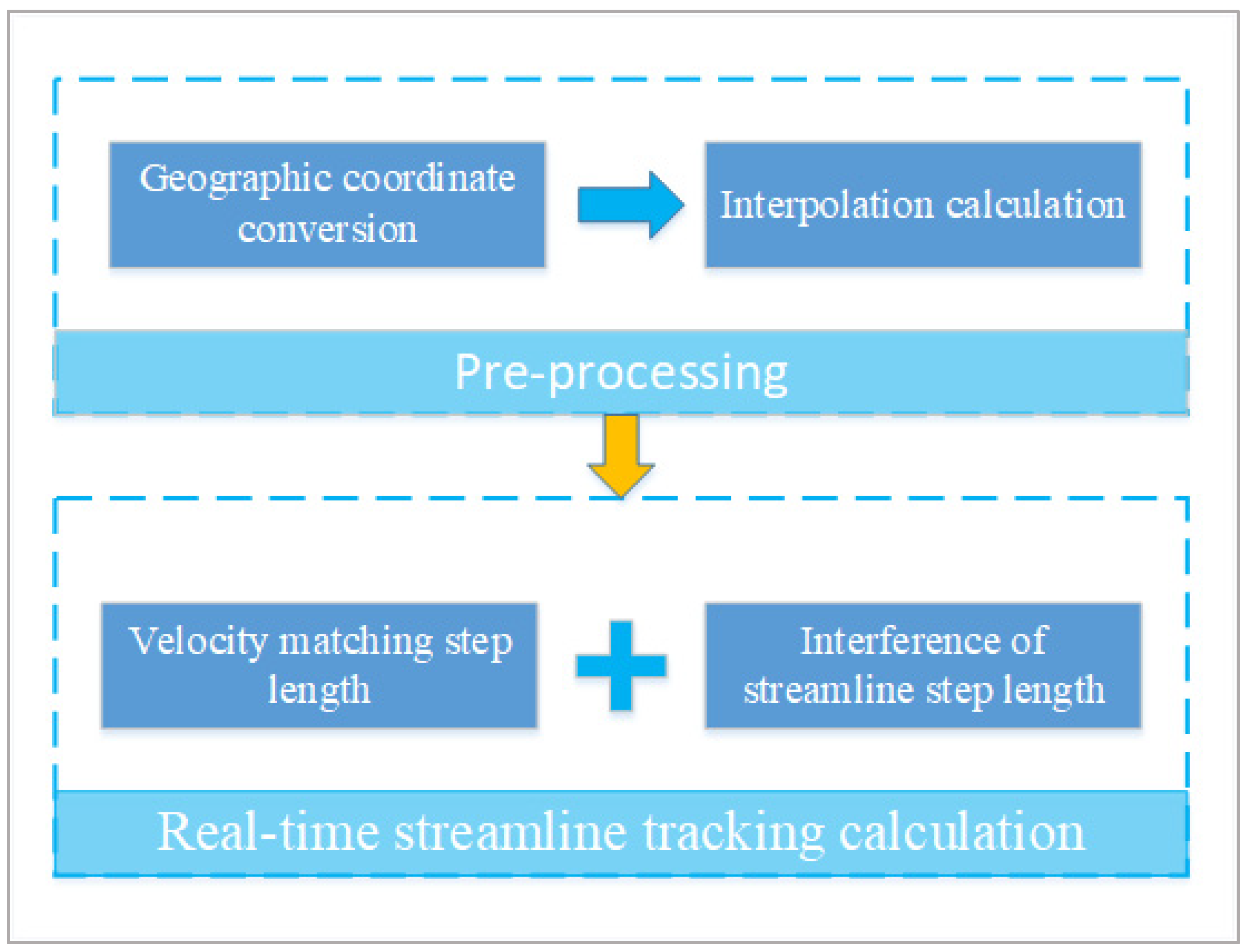
As shown in Figure 1, this algorithm is organized as follows. First, corresponding geographic coordinate points in ocean current data to the screen coordinate system, and then, performing interpolation calculations to ensure that all pixels within the screen area corresponding to the geographical extent of the data have values. Finally, using the integration algorithm that combines velocity matching and step length intervention to calculate streamline trajectories.

2.1.1. Geographic Coordinate Conversion and Interpolation Calculation

Unlike traditional drawing methods that work in the geographic coordinate system, this algorithm draws streamlines by operating with screen pixel units. Therefore, it is necessary to convert geographic coordinates to screen coordinates in this process. Besides, due to data sampling precision, some pixels within the screen area corresponding to the geographical extent of the data will be left with null values after the geographic coordinate system is converted to the screen coordinate system. Thus, an interpolation algorithm is also required.

• Geographic coordinate conversion

Common projection conversion algorithms include the transverse Mercator projection (UTM), Albers equal product Conic projection (Albers), Lambert Conformal Conic projection (Lambert Conic), Mercator projection (Mercator) and so on [11,12]. The Mercator projection is the most widely used projection algorithm in web two-dimensional visualization, but there is a problem that the more closer to the polar region, the more regional deformation it gets [13], which means the latitude lines are not evenly spaced on the map. Therefore, according to the reference [14], the inverse Gudermannian function [14] should be used to calculate the latitude line displacement from the equator on this projection, and then the coordinate range in the y direction can be figured out. Then with the help of radians, geographic coordinates can be easily converted to screen coordinates. The conversion formula is shown as follows.

$$project\left(lat,lon\right)=\{\begin{array}{l}mercY\left(\alpha \right)=\ln \left(\tan \left(\frac{\pi }{4}+\frac{\alpha }{2}\right)\right)\\ ymin=mercY\left(south\right)\\ ymax=mercY\left(north\right)\\ x=\left(rad\left(lon\right)-west\right)\ast \frac{Width}{\left(east-west\right)}\\ y=\left(ymax-rad\left(lat\right)\right)\ast \frac{Height}{\left(ymax-ymin\right)}\end{array}$$

(1)

In this formula $mercY$ is the y-coordinate calculation method in the inverse Gudermannian function, and $\alpha$ is the radian value of latitude in the geographic coordinate system, while $south$ and $north$ are the latitude radian values in the upper and lower boundaries of the visible map area. The screen coordinate range $ymin$, $ymax$ in the y direction can be calculated out according to the above conditions. Besides, $east$ and $west$ are the longitude radian values in the left and right boundaries of the visible map area, $Width$ and $Height$ respectively are the number of pixels in the screen width and height, $lat$ and $lon$ are respectively the longitude and latitude of the geographic point, while $rad$ is the latitude and longitude radian calculation function and $x$, $y$ are the conversion results.

2.

Interpolation algorithm

Commonly used interpolation algorithms include nearest neighbor interpolation, bilinear interpolation, bicubic interpolation and so on [15,16]. According to the literature [15], nearest neighbor interpolation has the advantages of simple implementation and fast computing, but the interpolation results are poor in data continuity. Bilinear interpolation guarantees the continuity and the overall effect of interpolation results. However, this algorithm is more complex than nearest neighbor interpolation, which decreases the calculation speed somehow. Bicubic interpolations are much better than bilinear interpolation in interpolation results, which makes it more time-consuming. Taking into consideration both the computing time and interpolation results comprehensively, the interpolation algorithm adopted in this paper is bilinear interpolation.

2.1.2. Real-Time Streamline Tracking Calculation

Commonly used streamline tracking algorithms include the Euler method, second-order Runge-Kutta method, and fourth-order Runge-Kutta method [17,18]. Generally, as the order of integral algorithm increases, the precision of calculation results and the computational requirements of the algorithm will also increase, which means as the visualization becomes better, the calculation speed will decrease. A practical online map system must be the unity of precision and speed [19]. So taking into consideration both the visualization and efficiency of streamline calculating, this paper chooses the first-order Euler method as the integral algorithm to perform these calculations, and the formula is as follows.

$$\mathrm{y}\left(\mathrm{t}+{\Delta }_t\right)=y\left(t\right)+{{\displaystyle \int }}_t^{t+{\Delta }_t}V\left(P\left(H\right),t\right)dt$$

(2)

In the formula, $V\left(P\left(H\right),t\right)$ represents the integrand of streamline integral algorithm, and $P\left(H\right)$ is streamline step length intervention function. H is the intervention intensity coefficient of streamline step length, and $y\left(t\right)$ stands for the position of streamline at the time t.

In the same scale level, streamline step length can be controlled by flow field velocity, the larger the velocity is, in unit time, the longer the streamline step length is, while in multi-scale levels, problems such as feature retention of the flow field and adaptive step length still need to be dealt with separately. Therefore, the step length intervention calculation function $P\left(H\right)$ and step length intervention intensity $H$ are introduced into the streamline integral function.

When the user scales an online map at different levels, the geographic extent displayed on the device will change accordingly, which will cause the line segment distance in the screen coordinate system corresponding to the two geographic coordinate points to change. For example, in Figure 2 there are three geographical coordinate points, A, B, and C, and when scaling the map from the large scale view to the small, the pixel intervals of line segments AB and AC will get shorter. Based on this phenomenon, a kind of multi-scale streamline step size intervention measure can be taken to optimize the multi-scale streamline expression effect.

In order to intervene the multi-scale streamline step length scientifically, the step length intervention coefficient must be calculated. Before this operation, the longitude and latitude of the tracking point should be offset by the step length intervention intensity coefficient $H$. Then, the difference in the line segment distances between the tracking point and the offset points can be figured out using Formula (3) to calculate the step length intervention coefficient. And the final data of the size and direction of the flow field can be calculated by using Formula (4).

$$P(H)=\{\begin{array}{l}\mathrm{h}\mathsf{\lambda }=\mathrm{lon}<0?\mathrm{H}:-\mathrm{H}\\ \mathrm{h}\mathsf{\phi }=\mathrm{lat}<0?\mathrm{H}:-\mathrm{H}\\ \mathrm{p}\mathsf{\lambda }=\mathrm{project}\left(\mathrm{lat},\mathrm{lon}+\mathrm{h}\mathsf{\lambda }\right)\\ \mathrm{p}\mathsf{\phi }=\mathrm{project}\left(\mathrm{lat}+\mathrm{h}\mathsf{\phi },\mathrm{lon}\right)\\ k=\cos \left(\frac{\mathrm{lat}}{360}\ast 2\ast \mathsf{\pi }\right)\\ d0=\frac{\left(p\lambda \left[0\right]-x\right)}{h\lambda }\frac{1}{k}\\ d1=\frac{\left(p\lambda \left[1\right]-y\right)}{h\lambda }\frac{1}{k}\\ d2=\frac{\left(p\phi \left[0\right]-x\right)}{h\phi }\\ d3=\frac{\left(p\phi \left[1\right]-y\right)}{h\phi }\end{array}$$

(3)

$$\{\begin{array}{c}U=d0\ast u+d2\ast v\\ V=d1<\ast u+d3\ast v\end{array},$$

(4)

In above formulas, $lon$ and $lat$ are respectively the longitude and latitude of the tracking point, while $h\lambda$, $h\phi$ are respectively the longitude and latitude after the increment. $p\lambda$ and $p\phi$ are respectively the screen coordinates of $h\lambda$ and $h\phi$. $project$ is the geographic coordinate conversion function, $k$ is the radian value of the latitude, and $x$, $y$ are the screen coordinates of the trace point. $d0$, $d1$, $d2$ and $d3$ are the streamline interference coefficients.

2.2. Grid + Feature Seed Point Placement Method

The visualization effect of geometric flow visualization method relies heavily on the location of seed points [1]. In order to solve the problem of uneven distribution of seed points, this paper proposes a double seed point placement strategy which contains a global regular grid distribution algorithm and a feature area random distribution algorithm.

• Global regular grid distribution algorithm: a method that achieve uniform layout by sampling screen pixels at equal intervals which means seed points are evenly distributed on a regular grid [20].
• Feature area random distribution algorithm: using the direct generation algorithm [2] to distribute seed points in the feature region which is extracted by using the flow field feature extraction method which proposed from literature [21].

2.3. Collision Detection Algorithm Based on Attribute Information Judgment

After the symbolization of geographical objects, instances of unreasonable covering between the symbols are referred to as conflicts [22]. Traditional collision detection methods generally adopt the operation flow of “symbolization first (see expression effect), and post-processing” [23]. When using this kind of method, the symbol graphs should be rasterized first, and some information such the raster numbers, raster occupiers, and occupation times, should be recorded to complete the rough collision detection. Then, geographic semantic analysis should be used to eliminate false conflicts. Finally, a complete list of conflicts between the symbols can be found [22]. Although this kind of method can accurately detect graph collisions, it has data redundancy in data storage, which affects the efficiency of online mapping.

In order to improve the drawing efficiency, this paper proposes a collision detection algorithm based on attribute information judgment which can detect and correct the conflicts before the streamlines are drawn [24]. By using this method, an operation flow of “processing first, then symbolization” [23], which performs well in terms of the efficiency of online mapping, can be realized. And this algorithm contains two parts.

2.3.1. Rough Detection of the Conflicts

Before detecting the conflicts, it is necessary to store the first drawing streamline into the non-conflict group. Then, the streamlines in the group are compared with others by looking at whether their encasing rectangles overlap, and updating the non-conflict group to include streamlines whose rectangles do not create new conflicts. Finally, the result of rough detection can be worked out. However, this result excludes two kinds of situations that are shown in Figure 3, so some measures should be taken to correct this.

The process of rough detection can be defined with Formula (5).

$$\mathrm{Conflict}=\{\begin{array}{l}{\left(\mathrm{line}1\mathrm{left},\mathrm{line}2\mathrm{left}\right)}_{\max }<{\left(\mathrm{line}1\mathrm{right},\mathrm{line}2\mathrm{right}\right)}_{\min }\\ {\left(\mathrm{line}1\mathrm{bottom},\mathrm{line}2\mathrm{bottom}\right)}_{\max }<{\left(\mathrm{line}1\mathrm{top},\mathrm{line}2\mathrm{top}\right)}_{\min }\end{array},$$

(5)

In this formula, $line1left$, $line2left$, $line1right$ and $line2right$ respectively represent the minimum and maximum x-coordinates of the starting point in streamline 1 and streamline 2, and, $line1bottom$, $line2bottom$, $line1top$ and $line2top,$ respectively, are the minimum and maximum y coordinate of the starting point in streamline 1 and streamline 2.

2.3.2. The Correction of the Rough Detection Result

During the correction process, the line segments based on the starting and ending points of each streamline in the non-conflict group need to be constructed, and then the Euclidean distance from starting and ending points of excluded streamlines to the line segments in the group are calculated. The minimum distance is compared to the given threshold value M, and the group is updated to include streamlines with a minimum distance greater than or equal to M. Finally, the result of non-conflicting streamlines can be found. This process can be defined with Formula (6).

$$\mathrm{Correction}={\left(\mathrm{distanceLeft},\mathrm{distanceRight}\right)}_{\min }>\mathrm{M},$$

(6)

In this formula, $distanceLeft,distanceRight$ respectively are the Euclidean distance from starting and ending points of streamline 1 to streamline 2, and M is the given distance threshold which values a quarter of the combined length of the longest and shortest streamlines.

3. Experiments

In this section, a series of experiments are carried out to evaluate the relevant algorithms used in this paper and to compare different mapping algorithms. Besides, the flow field data is provided by ECMWF (European Centre for Medium—Range Weather Forecasts).

3.1. Experiments About Seed Point Placement Methods

3.1.1. The Uniformity of Global Regular Grid Distribution Algorithm

The uniformity of a finite point set is an evaluation criterion for the equilibrium degree of points in a parameter space [2]. In order to evaluate the uniformity of the global regular grid distribution algorithm, this paper does some experiments using the improved uniformity deviation measurement method proposed in the literature [25]. This measurement method can be defined as follows.

Definition 1.

Suppose there is an m-dimension cube $C^m={\left[0,1\right]}^m$, and point set $\mathrm{A}=\left\{x_1,x_2,\dots ,x_n\right\}$ belongs to m.

Then

$$\overline{\mathrm{x}}=\frac{1}{n}{\displaystyle {\displaystyle \sum }_{i=1}^n}{x}_i$$

(7)

$$R^2=\frac{1}{n}{\displaystyle {\displaystyle \sum }_{i=1}^n}{\left(x_i-\overline{x}\right)}^{’}\left(x_i-\overline{x}\right)=\frac{1}{n-1}{\displaystyle {\displaystyle \sum }_{i=1}^n}d\left(x_i,\overline{x}\right)$$

(8)

$$\mathrm{E}\left(\mathrm{A}\right)=\frac{\underset{y\in C^m,1\le k\le n}{\sup min}d\left(y,X_k\right)}{R}$$

(9)

In the above formulas, $d\left(y,X_k\right)$ denotes the Euclidean distance between $y$ and $X_k$, and $y\in C^m,1\le k\le n$. Additionally, $\sup mind\left(y,X_k\right)$ represents the maximum value of the minimum Euclidean distance in finite point set A, while $E\left(A\right)$ stands for the uniformity of finite point set A. For this latter measure, smaller values are better [2,26].

For the convenience of calculation, in this experiment, global regular grid distribution algorithm and two commonly used seed point placement algorithms which include the direct generation algorithm and Sobol sequence algorithm [2,27,28] are used to generate 2500 points in two-dimensional space $C^2={\left[0,1\right]}^2$.

3.1.2. Efficiency Comparison of Seed Point Placement Algorithms

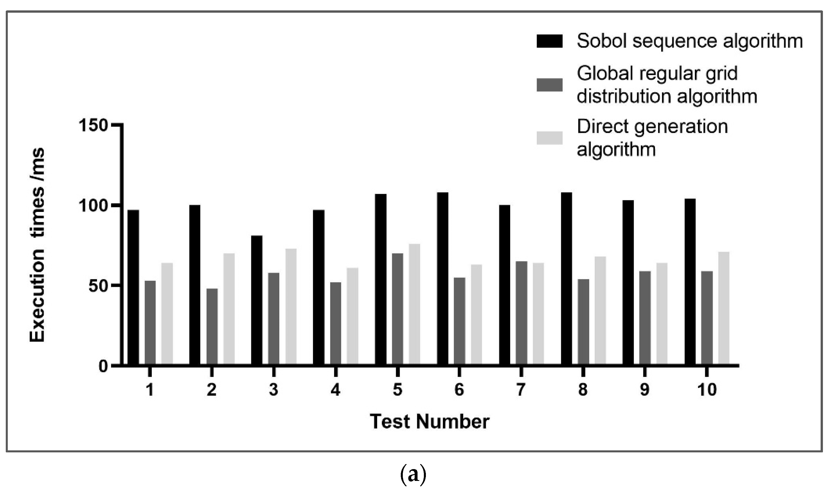
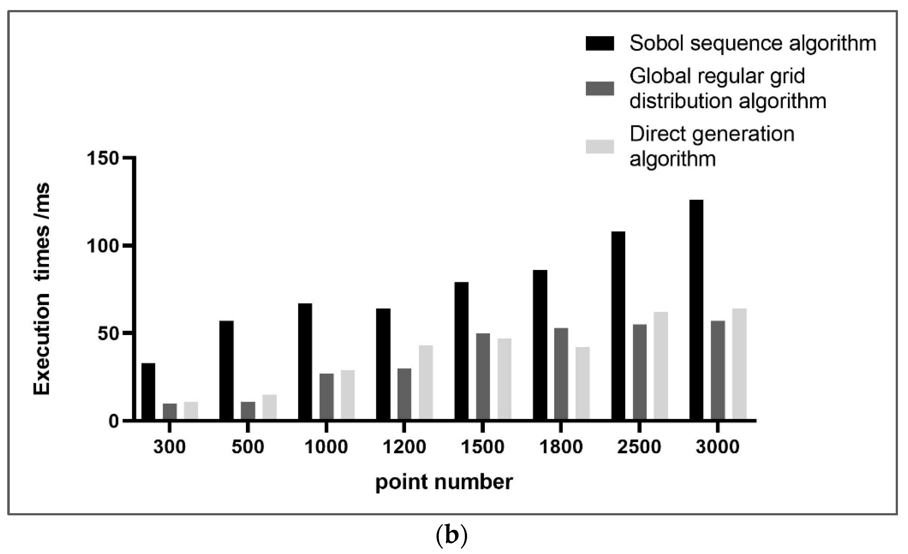
Algorithm efficiency is generally used to describe the execution time of the algorithm. In this section, this paper compares the algorithm efficiency of direct generation algorithm, Sobol sequence algorithm and global regular grid algorithm. To make the experimental data more convincing, this section carries out two groups of algorithm efficiency comparison experiments on the basis of Section 3.1.1. The two groups’ experiments are both generate points in two-dimensional space $C^2={\left[0,1\right]}^2$. But, the difference is that in one set of experiments, the three algorithms are respectively generate 2500 points in space $C^2$, while in another, the three algorithms are respectively generate eight groups’ different numbers of points in space $C^2$.

3.1.3. Rendering Effect Comparison of Seed Point Placement Algorithms

In this section, direct generation algorithm, Sobol sequence algorithm, global regular grid distribution algorithm, and double seed point placement method are used to compare their rendering effects. Before this operation, the feature regions should be extracted to meet the calculation requirements of double seed point placement method.

According to flow field feature extraction algorithms which have been proposed in literature [21], steps such as the eddy current feature region analysis, spatial autocorrelation analysis of flow velocity, velocity classification processing, spatial autocorrelation analysis of flow direction rate, and flow direction rate classification processing should be carried out first when extracting the features, and then the weight assignment results of the above steps should be sequentially calculated. Finally, the feature weight of the flow field data can be determined by using the attribute weighting method based on rough set theory and the extraction result can be obtained.

By using these theories and algorithms, this paper extracts the flow field features from the ocean current data and visualizes the data with above seed point placement algorithms. Besides, in this experiment, the sampling interval is set to 20 for both global regular grid distribution algorithm and double seed point placement method.

3.2. Experiments About Mapping Method Proposed Herein

To perform those experiments, first, Leaflet is chosen as the map rendering engine for its simplicity, performance, and usability [29]. Then, feature streamlines should be calculated by using those theories proposed herein, and next, Canvas visualization technology is selected to draw streamlines for its fast render speed and less consumption of memory [11]. Then this prototype system [30] can realize flow field dynamic real-time drawing [31].

Based on the above techniques, this paper visualizes the experimental flow field data and mapping the same ocean current vortex at four scales to compare the situation of feature retention at each scale. Meanwhile, to compare this mapping method better, this paper utilizes the direct flow visualization method, geometric flow visualization method, and multi-scale flow field mapping method based on real-time feature streamlines to visualize the same flow field data. Besides, in this experiment, the sampling interval used in double seed point placement method and the direct flow visualization method is 20.

3.3. Experiments About Map Load

Map load is an important indicator for evaluating a map [32,33,34]. In order to maintain balance at different scales, this paper proposed a formula to calculate the sampling interval of the global regular grid distribution algorithm.

$$\mathrm{I}=\mathrm{c}+\mathrm{level}\ast \mathrm{scale},$$

(10)

In this formula, $c$ is a constant of basic sampling interval, $level$ is the difference between the current map zoom level and the minimum map zoom level, and $scale$ is an equilibrium parameter for multi-scale sampling.

In order to identify the map load balance condition, this paper needed to find out the relationship between the map scale level and the radian value of geographical range area. Formula (11) is proposed to calculate the radian value of geographical range area.

$$\mathrm{Area}=\left(\mathrm{West}-\mathrm{East}\right)\ast \left(\mathrm{North}-\mathrm{South}\right),$$

(11)

In the formula, $West$ is the radian value of the longitude to the left of the visible region, $East$ is the radian value of longitude to the right of the visible region, $Nort\mathrm{h}$ is the radian value of latitude to the top of visible region, and $South$ is the radian value of latitude to the bottom of visible region.

To determine the appropriate value of basic sampling interval and equilibrium parameter for multi-scale sampling used in Formula (10) and balance the map load, the following experiments are required. First, by using Formula (11), the radian values of geographical range area from zoom level 3 to 10 can be calculated, and then the area ratio between adjacent scaling levels can be obtained by operating those data. Next, an approximate value of the equilibrium parameter for multi-scale sampling can be found by using the relationship between the map scale level and the radian value of geographical range area. And then, another experiment should be carried out to verify the correctness of this approximate value. Finally, with the experimental results for different basic sampling interval and map load, the basic sampling interval can be determined by using the theories in literature [21] and literature [35].

4. Results

4.1. Results for Uniformity Evaluation

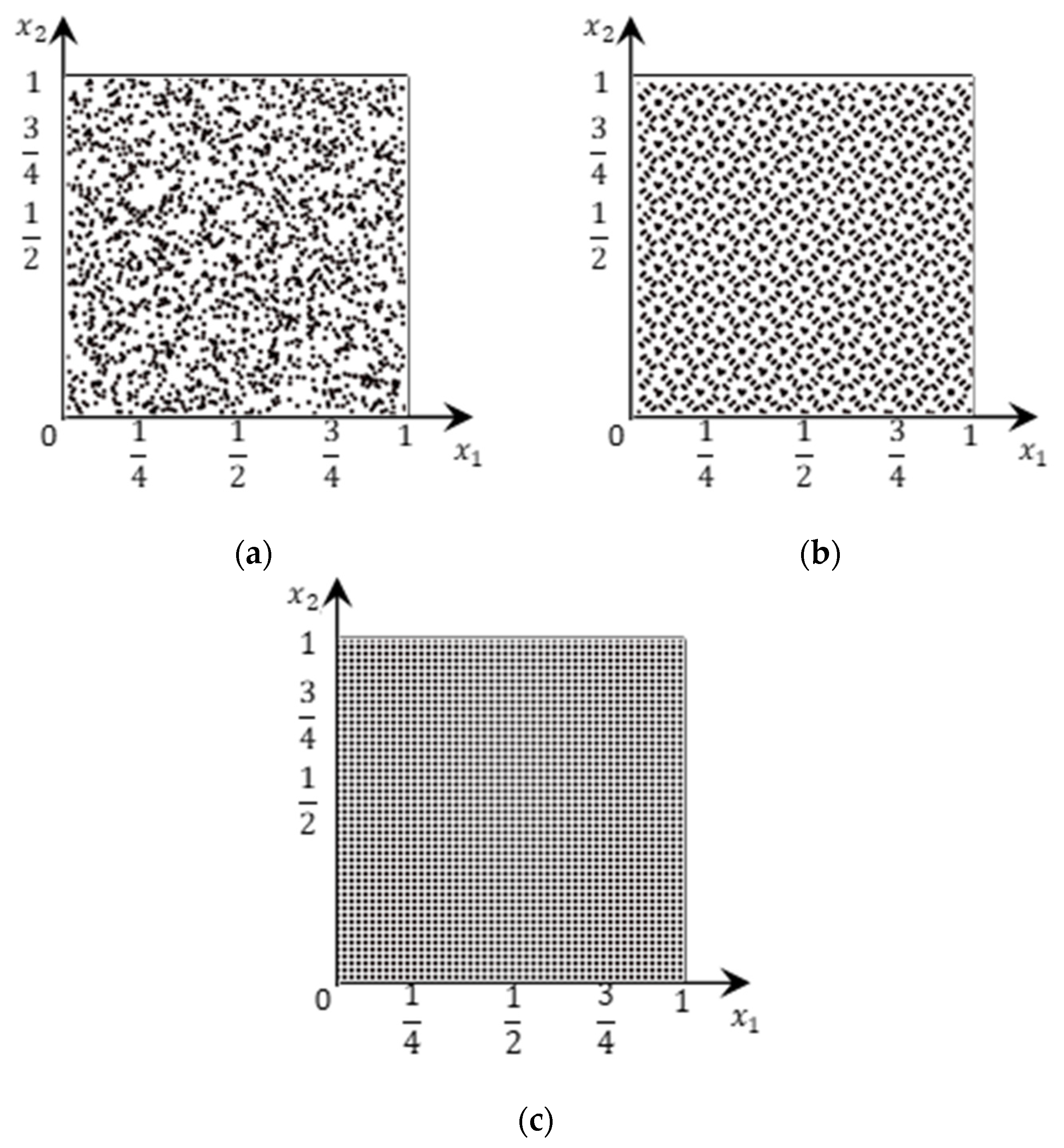
Figure 4 shows the distribution maps of the three kinds of seed point placement algorithms in two-dimensional space $C^2={\left[0,1\right]}^2$. By using Formulas (7)–(9), the uniformities of the direct generation algorithm, Sobol sequence algorithm, and global regular grid distribution algorithm respectively are $\mathrm{E}\left(\mathrm{a}\right)=$ 0.0835, $\mathrm{E}\left(\mathrm{b}\right)=$ 0.0536 and $\mathrm{E}\left(\mathrm{c}\right)=$ 0.0457.

4.2. Results for Algorithm Efficiency Comparison

In this section, the efficiency of three algorithms is compared from two aspects, And Figure 5 shows the schematic diagrams of three algorithms’ efficiency comparison results.

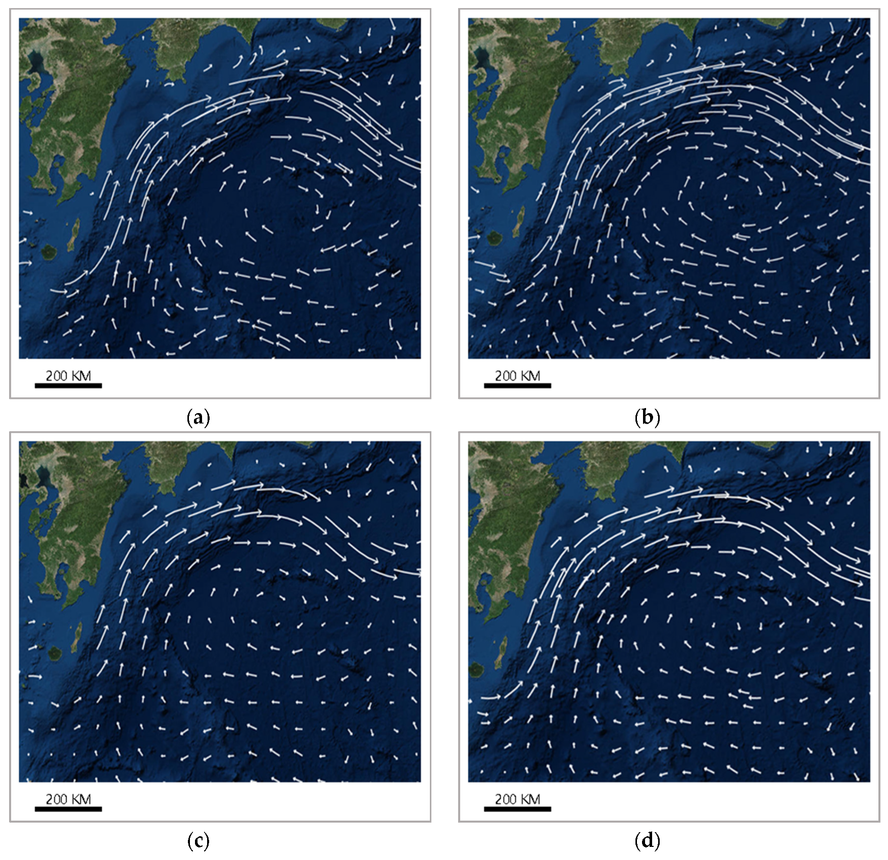
4.3. Results for Rendering Effect Comparison

Figure 6 is the schematic diagram of feature extraction result. In the figure, different color represents different kind of feature area. And Figure 7 is the cartographic renderings of four point placement methods.

4.4. Results for Multi-Scale Mapping Expression Effect

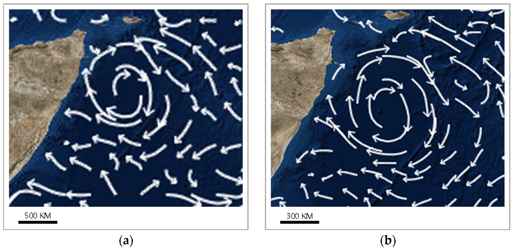
Figure 8 shows the expression renderings of flow field eddy currents at different scales by using multi-scale flow field mapping method based on real-time feature streamlines.

4.5. Results for Different Mapping Method Expression Effect

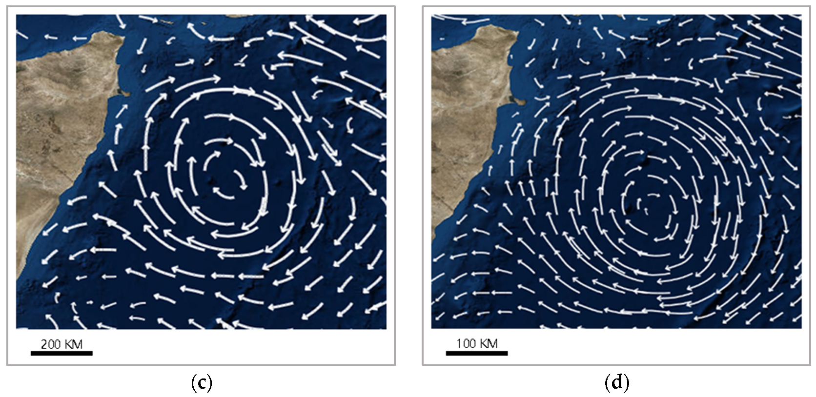
Figure 9 is the flow field eddy current effect diagrams for direct flow visualization method, geometric flow visualization method, and multi-scale flow field mapping method based on real-time feature streamlines.

4.6. Results for Map Load Experiments

Table 1. Corresponding table of zoom level and the radian values of geographical range area.

Zoom Level	Radian Value of Geographical Range Area
3	13.166
4	3.961
5	1.049
6	0.266
7	0.067
8	0.017
9	0.004
10	0.001

is the experimental results about radian values of geographical range area from zoom level 3 to 10 which calculated by Formula (11).

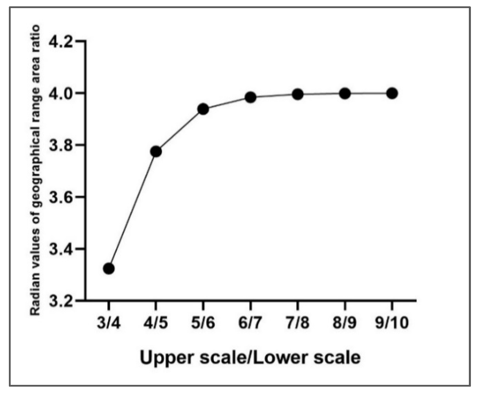
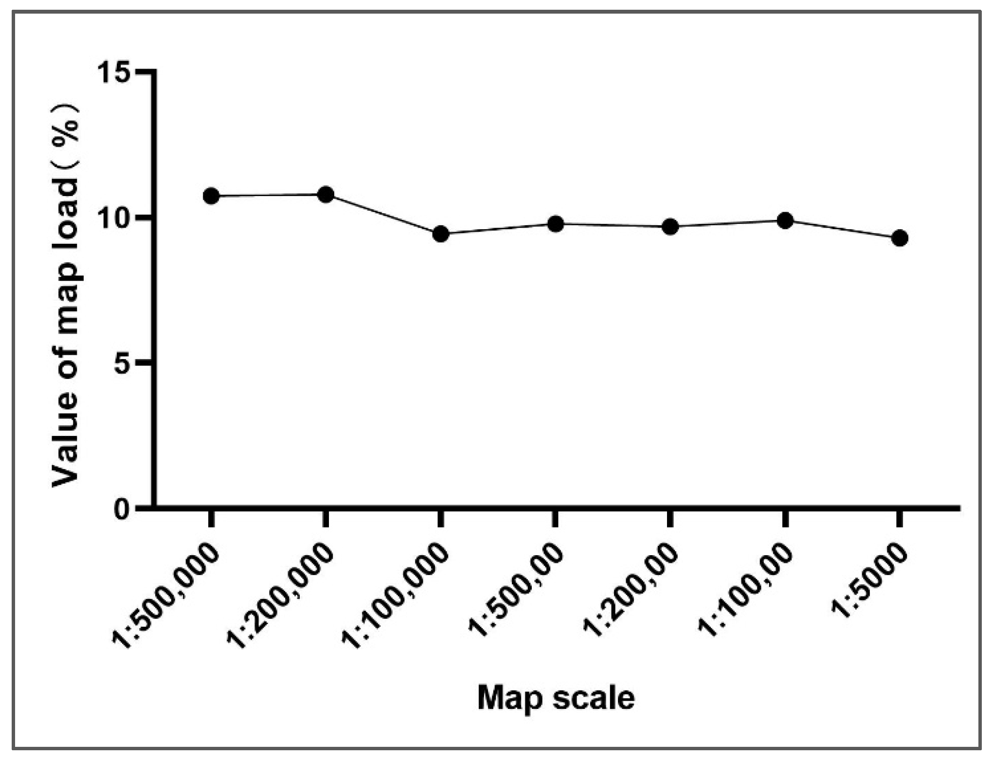
The results in

Table 2. Table of radian values of geographical range area ratio.

Upper Scale/Lower Scale 1	Radian Values of Geographical Range Area Ratio
3/4	3.324
4/5	3.775
5/6	3.939
6/7	3.984
7/8	3.996
8/9	3.999
9/10	4.000

¹ Upper scale/Lower scale means Upper scale divided by Lower scale.

is calculated from Table 1. And Figure 10 is the line chart of radian values of geographical range area ratio that drawn according to Table 2. With this corresponding relationship table, the approximate value of equilibrium parameter for multi-scale sampling can be determined to be 4. Meanwhile,

Table 3. Corresponding table of map scale and value of map load.

Map Scale	Value of Map Load (%)
1:500,000	10.743
1:200,000	10.790
1:100,000	9.435
1:500,00	9.779
1:200,00	9.688
1:100,00	9.896
1:5000	9.295

is the experimental data for verify the correctness of this equilibrium parameter value for multi-scale sampling, and Figure 11 is line chart of map scale and value of map load.

Table 4. Corresponding table of basic sampling interval and map load.

Basic Sampling Interval	Value of Map Load (%)
5	74.472
10	71.213
12	40.428
13	32.245
14	26.202
15	21.721
16	18.609
17	16.118
20	10.743
25	6.297

shows the results of corresponding relationship between the value of map load and different basic sampling intervals at the map scale of 1:500,000.

5. Discussions and Conclusions

According to the results in Section 4.1 and theories in the literature [25], the global regular grid distribution algorithm is better than the direct generation algorithm and the Sobol sequence algorithm in the mathematical evaluation of uniformity.

According to Figure 5, it can be concluded that the algorithm efficiency of global regular grid distribution algorithm is the highest one among the three. Sobol sequence algorithm is the least efficient of the three, and the algorithm efficiency of direct generation algorithm is second only to global regular grid distribution algorithm.

By comparing the renderings in Figure 7, it can be concluded that the distribution uniformity of Sobol sequence algorithm is better than direct generation algorithm, but both of them display the phenomenon of streamline vacancy in the mapping region. Besides, the seed point placement algorithms used in Figure 7c,d are more uniform in visual effect than those used in Figure 7a,b, Moreover, by comparing Figure 7c,d, it can be concluded that the distribution density in the feature regions that are drawn by the double seed point placement method is higher than when the global regular grid algorithm is used.

Analysis of those algorithms can reveal that the direct generation algorithm belongs to the class of pseudo-random generation algorithms [36] and that, because of the randomness, it is easy to end up with local clustering phenomena in the cartographic area [37]. Meanwhile, the Sobol sequence algorithm uses quasi-random sequences [38] which sacrifice randomness to retain the uniformity of distribution [39], so it is easy to end up with overly-prominent regularity in streamline drawing. Though the global regular grid distribution algorithm is better in distribution uniformity, it still has many problems. For example, sampling screen pixels at equal intervals not only improves the distribution uniformity, but also weakens the expression of feature areas, which will cause the illusion of uniform velocity in the whole flow field for users [40]. Besides, this method also causes overly prominent regularity in streamline drawing. Therefore, it is needed to combine two different seed point placement algorithms to express the flow field.

Taking into consideration algorithm efficiency of those methods, this paper uses global regular grid distribution algorithm to ensure the uniformity of seed point placement and generates random points in feature areas with direct generation algorithm. Since the seed points have been evenly distributed by using global regular grid distribution algorithm and the direct generation algorithm is only used in the feature areas, the defects of the two algorithms are compensated for each other. Therefore, the double seed point placement method can express the flow field features better.

According to the results in Section 4.4, it can be concluded that the mapping method proposed herein is helpful for multi-scale cartography. Moreover, according to Figure 9, it can be seen that the direct flow visualization method can roughly express the structure of the flow field eddy current with arrows and colors. However, a single arrow and color can only represent the information of one location in the flow field, which ignores the continuity of the vector field. Additionally, it is easy to produce an illusion of uniform velocity in the whole flow field by using the same sampling interval in the whole vector field. The geometric flow visualization method can express the flow field by using long streamlines, which can show the global continuity of the flow field easily. However, the flow direction information is hard to determined [3], and unreasonable covering between long streamlines, which results in a messy drawing, is obvious. The method presented in this paper retains the arrow pointing and color coding used in the direct flow visualization method, which makes it easier to identify the flow direction in the flow field. Additionally, by using the collision detection algorithm, visual confusion in the drawing results is avoided.

With the data in Table 1 and Table 2, it can be seen that the radian value of the geographical range area ratio is infinite close to 4. And according to this relationship, when set 4 as the equilibrium parameter for multi-scale sampling and set 20 as the basic sampling interval, the data in Table 3 shows that the value of the map load at around 10% at different scales, which indicates that the map load reaches equilibrium. Meanwhile, with the data in Table 4 and the theories in literature [21], it can be concluded that to reach the appropriate value of map load, the basic sampling interval which used in Formula (10) should be controlled between 14 and 16.

In conclusion, the mapping method proposed in this paper, which primarily includes a real-time streamline tracking algorithm based on a screen coordinate system, a stable double seed point placement method that contains a global regular grid distribution algorithm and a feature area random distribution algorithm, and a collision detection algorithm based on attribute information judgment, is more uniform in terms of seed point distribution and expresses the feature areas of flow field more obviously. In addition, the collision detection algorithm based on attribute information judgment can help to detect and handle the conflicts before symbolization which will improve the efficiency of online drawing and avoid messy visualization. However, there are still some unsolved problems in this paper which need to be researched. For example, the relationship between the sea and land is ignored when using the global regular grid distribution algorithm. So, in future research, more schemes should be used to solve these known problems. Besides, the described algorithm and online demo can be fetched from the website http://onlinemap.xyz/, and it would be useful for users to evaluate and compare them with other flow field visualization methods.

References

- Li, C.X.; Peng, R.C.; Gao, Z.S. An Improved Legible Method for Visualizing 3D Flow Field. Geomat. Inf. Sci. Wuhan Univ. 2017, 42, 744–748. [Google Scholar]
- Fang, J.; Ai, B.; Xin, W.P.; Shang, H.S. Dynamic flow field expression optimization method based on particle system. Sci. Surv. Mapp. 2018, 43, 72–76. [Google Scholar]
- Wang, S.B.; Pan, Z.G. Comparison, Analysis and Review of 2D Flow Visualization. J. Syst. Simul. 2014, 26, 1875–1881. [Google Scholar]
- Zheng, L.T. Research and Implementation of Feature-Based Streamline Selection Method for Flow Field. Master’s Thesis, National University of Defense Technology, Changsha, China, 2015. [Google Scholar]
- Ba, Z.Y.; Shan, G.H.; Liu, J. A Feature-Based Seeding Method for Multi-Level Flow Visualization. J. Comput. Aid Desig. Comput. Graph. 2016, 28, 32–40. [Google Scholar]
- Shen, W.H.; Wang, S.B.; Pan, Z.G. New 2D Flow Visualization Method Based on Mutual Information and Image Fusion. J. Syst. Simul. 2015, 8, 1796–1800. [Google Scholar]
- Liao, Z.Y. The Research of Spatio-Temporal Feature Analysis and Visualization on Marine Flow Field Based on Topological Theory. Master’s Thesis, Shandong University of Science and Technology, Shandong, China, 2017. [Google Scholar]
- Liao, Z.Y.; Ji, M. Comparison, Analysis of 3D Marine Flow Visualization. Geomat. Spat. Inf. Technol. 2016, 113, 107–109. [Google Scholar]
- Huang, D.M.; Du, Y.L.; Zhang, L.W. Two information entropy based seeding methods for 3D flow visualization. Comput. Eng. Sci. 2018, 40, 411–417. [Google Scholar]
- Tian, D.; Chi, X.B.; Wang, T.Q. Flow field visualization method based on weighted random sampling. Comput. Eng. Des. 2018, 1, 12. [Google Scholar]
- Ma, Z.J. Research and Implementation of Atmospheric Data Visualization system Based on Web. Master’s Thesis, Hangzhou Dianzi University, Hangzhou, China, 2017. [Google Scholar]
- Sun, L.D. Gauss-Kruger Projection and Universal Transverse Mercator projection of the Similarities and Differences. Port Eng. Technol. 2008, 5, 51–53. [Google Scholar]
- Wang, H.B.; Zhang, H.W.; Zhang, P.P. A Transverse Mercator Chart Suitable for Polar Regions. Chin. J. Polar Res. (Chin. Ed.) 2017, 29, 454–460. [Google Scholar]
- Gudermannian Function. Available online: https://en.wikipedia.org/w/index.php?title=Gudermannian_function&oldid=856643283 (accessed on 7 June 2019).
- Deng, C. Research of Image Interpolation Algorithm. Master’s Thesis, Chongqing University, Chongqing, China, 2010. [Google Scholar]
- Ding, X.J. Research and comparison of Matlab interpolation algorithm for image scaling function. J. Hubei Univ. (Nat. Sci.) 2018, 40, 396–400. [Google Scholar]
- Ji, M.; Chen, L.; Yan, F.X. The Adaptive-Step-based Marine Fluid Flow Streamline Constructing Algorithm. Geomat. Inf. Sci. Wuhan Univ. 2014, 39, 1052–1056. [Google Scholar]
- Wang, J.G.; Lian, R.M.; Xing, B. Streamline visualization method based on runge kutta fourth order integral. Wirel. Internet Technol. 2015, 13, 130. [Google Scholar]
- Yu, Z.Y.; Wang, Y.J.; Chen, X.G. The Model Design for Linear Dynamic Annotation Visualization in Digital Map. Acta Geogr. Sin. 2001, 56, 73–77. [Google Scholar]
- Jobard, B.; Lefer, W. Unsteady flow visualization by animating evenly-spaced streamlines. Comput. Graph. Forum 2000, 19, 31–39. [Google Scholar] [CrossRef]
- Ai, B.; Liu, Y.; Wang, Z.; Sun, D.C. Evaluation of multi-scale representation of ocean flow fields using the Euler method based on map load. J. Spat. Sci. 2019, 64, 1–13. [Google Scholar] [CrossRef]
- Yang, Y.; Li, L.; Wang, H. Method for improving precision of building subsidence observation. J. Geomatics. 2007, 32, 46–48. [Google Scholar]
- Li, L.; Yu, Z.H.; Zhu, H.H. Handling Graphic Conflicts between Cartographic Features: Exemplifying Geo-linear Features (Road, River and Boundary). Acta Geod. Cartogr. Sin. 2015, 44, 563–569. [Google Scholar]
- Li, S.Y.; Wang, L.J.; Cao, Y.N. Review of Automatic Identification Methods of Vector Map Data Defects. Surv. Mapp. Geol. Miner. Resour. 2015, 31, 1–4. [Google Scholar]
- Liu, Y.; Zhang, Z.; Ma, E.L. Some Methods of Measuring the Uniform Character of Finite Point Sets. J. Cap. Norm. Univ. (Nat. Sci. Ed.) 1997, 1997, 10–14. [Google Scholar]
- Zhu, Y.C. The Accurate Calculation Formula of Low-Dimensional Finite Point Set Deviation (III). Chin. Sci. Bull. 1994, 39, 1724–1725. [Google Scholar]
- Pan, J.J.; Li, Z.M. An improved algorithm of fast line integral convolution with Sobol sequence. J. China Univ. Pet. (Nat. Sci. Ed. 2007, 31, 162–166. [Google Scholar]
- Gu, D.W.; Ling, J. Improved novel Particle Swarm Optimization algorithm. Comput. Eng. Appl. 2011, 47, 49–51. [Google Scholar]
- Leaflet. Available online: http://leafletjs.com/ (accessed on 15 February 2019).
- Jiang, W.; Liu, L.K. Application of Prototype System in Software Development. Comput. Technol. Dev. 2019, 29, 110–115. [Google Scholar]
- Wu, F.Y. Application of Drawing Technology based on HTML5 Canvas. Electron. Test 2018, 4, 57. [Google Scholar]
- Sun, Q.H.; Jiang, N. Research on Electronic Map Load Calculation Model and Its Application. Bull. Surv. Map. 2014, 9, 54–57. [Google Scholar]
- Jiang, N.; Cao, Y.N.; Sun, Q.H. Exploration of two-peak changing law of basic electronic map load. Acta Geod. Cartogr. Sin. 2014, 43, 306G313. [Google Scholar]
- Wang, H.F.; Hua, Y.X.; Zhang, X.N. Research on the Method of Electronic Map Load Computing Based on Sense of Vision. Geomat. Spat. Inf. Technol. 2017, 40, 25–29. [Google Scholar]
- Jiang, N.; Zhang, W.; Cao, Y.N. A computational method of information load on electronic map based on RGB feature extraction. Surv. Mapp. Eng. 2013, 22, 39–42. [Google Scholar]
- Jin, B.D. Thinking about one type random number generation in JAVA. Inf. Technol. 2012, 2012, 181–183. [Google Scholar]
- Deng, Q.L.; Jiang, Z.G.; Han, S. Reliability Analysis of dustproof Water Supply Network System Based on Sobol. J. Tianjin Univ. (Sci. Technol.) 2018, 9, 005. [Google Scholar]
- Xu, L. A Simulation Study on Economic Dispatch of Electrical Power Systems Based on the A Quantum Behaved Particle Swarm Optimization. Master’s Thesis, Xi’an University of Science and Technology, Xi’an, China, 2013. [Google Scholar]
- Wang, S.H.; Zhang, Y.D.; Wu, L.N. Comparison of Pseudo-random Numbers and Quasi-random Numbers. Comput. Inf. Technol. 2010, 2010, 32–36. [Google Scholar]
- Yan, T.H.; Feng, C. Research and Implement for Flow Field based on streamline technique. Inf. Technol. Informatiz. 2018, 2008, 51–53. [Google Scholar]
Figure 1.
Workflow of real-time streamline tracking algorithm based on screen coordinate system. The real-time streamline tracking algorithm combines velocity matching and step length intervention to adaptive the streamline step length in multi-scale.
Figure 2.
Schematic diagram of multi-scale streamline step length intervention. Point A is a streamline tracking point, point B is generated by point A after latitude increment, and point C is generated by point A after longitude increment, besides, the increment values are both equal step length intervention intensity coefficient .
Figure 3.
Schematic diagram of two kinds of streamline encased rectangular covering situation. The left image represents a case where the streamlines do not conflict, and it should not be excluded. The right-hand image is one that represents conflict, and it should be excluded.
Figure 4.
(a) is the distribution map for the direct generation algorithm, (b) is the distribution map for the Sobol sequence algorithm, and (c) is the distribution map for the global regular grid distribution algorithm.
Figure 5.
Schematic diagrams of three algorithms’ efficiency comparison results. The two groups’ experiments are both generate points in two-dimensional space . In (a), the three algorithms are respectively generate 2500 points in space , while in (b), the three algorithms are respectively generate eight groups’ different numbers of points in space .
Figure 6.
The areas where the color is red or orange are the feature areas of the flow field data. While the blue areas indicate the land parts, and the yellow areas stand for the place where the flow field features are not obvious. Besides, the red frame selected area is the place where the rendering effects are compared in Section 3.1.3.
Figure 7.
(a) is the rendering of the direct generation algorithm. (b) is the rendering of Sobol sequence algorithm. While (c) is the rendering of the global regular grid distribution algorithm, and (d) is the rendering of double seed point placement method.
Figure 8.
(a) is an eddy current representation at 1:500,000 scale, and (b) is an eddy current representation at 1:300,000 scale, (c) is an eddy current representation at 1:200,000 scale, and (d) is an eddy current representation at 1:100,000 scale.
Figure 9.
Flow field eddy current effect diagrams generated by three different mapping methods at the map scale of 1:100,000. (a) is the rendering for the direct flow visualization method and the different color represents different ranges of velocity, (b) is the rendering for the geometric flow visualization method, and (c) is the rendering for the multi-scale flow field mapping method based on real-time feature streamlines, the different color stands for different ranges of velocity.
Figure 10.
The horizontal axis represents Upper scale divided by Lower scale, and the vertical axis represents the radian values of geographical range area ratio.
Figure 11.
Line chart of map scale and value of map load. The horizontal axis represents map scale, and the vertical axis represents the value of map load.