GEOBIA Achievements and Spatial Opportunities in the Era of Big Earth Observation Data

Abstract

The primary goal of collecting Earth observation (EO) imagery is to map, analyze, and contribute to an understanding of the status and dynamics of geographic phenomena. In geographic information science (GIScience), the term object-based image analysis (OBIA) was tentatively introduced in 2006. When it was re-formulated in 2008 as geographic object-based image analysis (GEOBIA), the primary focus was on integrating multiscale EO data with GIScience and computer vision (CV) solutions to cope with the increasing spatial and temporal resolution of EO imagery. Building on recent trends in the context of big EO data analytics as well as major achievements in CV, the objective of this article is to review the role of spatial concepts in the understanding of image objects as the primary analytical units in semantic EO image analysis, and to identify opportunities where GEOBIA may support multi-source remote sensing analysis in the era of big EO data analytics. We (re-)emphasize the spatial paradigm as a key requisite for an image understanding system capable to deal with and exploit the massive data streams we are currently facing; a system which encompasses a combined physical and statistical model-based inference engine, a well-structured CV system design based on a convergence of spatial and colour evidence, semantic content-based image retrieval capacities, and the full integration of spatio-temporal aspects of the studied geographical phenomena.

1. Spatial Image Analysis

1.1. Space First … or Never?

“Space matters …” is the condensed opening statement of the European Space Policy [1], highlighting the strategic importance of space infrastructure, also referred to as space capacity, with its three sub-systems: satellite-based (i) communication, (ii) navigation, and (iii) Earth observation (EO). When focusing on EO imaging systems, we suggest that ‘space matters’ also refers to the importance of geographic space as an underlying principle of the phenomena observed and monitored by EO satellites and related remote sensing (RS) techniques. By building on both aspects—space technology and spatial concepts—this article aims to place classic geographic object-based image analysis (GEOBIA) ideas within the viewpoint of big EO data. It has been written with the ambition to unify merits from the computer vision (CV) and the GIScience/GEOBIA communities, believing that the successful exploitation of the massive big Earth data requires communities and perspectives to converge. Only then, may we be able to fully understand, how such complex information and insight can be revealed and extracted from EO imagery. To learn from the requirements of big data analytics in general means to recognize their challenges and to scale up from case-based solutions to the ubiquitous. To achieve this, we follow an inter-disciplinary approach under the umbrella of cognitive science as a meta-discipline including philosophical and epistemological aspects. We also include CV as machine-based scene-from-image reconstruction, that builds on its past/current implementations of convolutional neural networks and deep learning, as well as its evolution within the sub-field EO satellite image understanding—see Section 1.2. In a complementary manner, GIScience provides methods and strategies on how to move from numeric, sub-symbolic raster data to discrete spatial units with symbolic meaning in several scaled representations. We suggest that both disciplines, CV and GIScience, need to respect the ultimate benchmark [2] and currently the only measure [3], namely human cognition, be it human/biological vision or the conceptual understanding [4] of our multidimensional world in simplified planimetric image representations.

As we initiate this dialogue, we deliberately use the term spatial image analysis [5]—even if it sounds somewhat tautological (as image analysis never happens space-less)—to emphasize the need to explicitly consider spatial concepts in image analysis. The term ‘spatial’ encompasses context-sensitive aspects, i.e., neighbourhood analysis, geometric aspects of spatially defined image primitives [6], such as size and form, as well as topological and non-topological aspects. Traditionally, spatial concepts have been incorporated in image pre-processing routines by using the mathematical operation of convolution (filtering, see also Section 2.3). Filters are neighbourhood operators, which in GIScience are referred to as focal operators in the domain of map algebra [7]. As the term ‘focal’ indicates, a filter’s kernel defines the spatial context in the immediate neighbourhood of a pixel. Today, filters are prominently employed by deep learning approaches for image analysis, in particular convolutional neural networks (CNN), where an interconnected network of hierarchical filters are used to represent and detect geographical features through machine learning techniques. Filter-based operators are well defined according to neighbourhood type (e.g., 4- or 8-neighbors), kernel size, and pixel resolution. On the other hand, they remain per-pixel operators in the sense of a moving window, acting independently of the scene content and the type of geographic features represented in an image.

Owing, however, to the fact that digital imagery is not just organised in pixel arrays, but at the same time we observe the strong prevailing effect of image-related spatial autocorrelation (see Section 3.2), pixel grouping (i.e., multiscale regionalization) and, more specifically, image segmentation techniques have gained popularity, especially when dealing with very high (spatial) resolution (VHR) EO image data. Segmentation, preferably in several nested scales, is a key concept in the GEOBIA paradigm (Section 3) [8,9]. Singular pixels (i.e., picture elements) are individual Earth-surface observations at a specific location with relative or absolute, real-world coordinate-tuples. Still, as 0D representations [10] they do not carry any spatial property in addition to their relative or absolute location, and brightness and/or colour value. Conversely, human vision behaves diametrically different: that is, we can only interpret and understand images once individual pixels are ignored and spatially aggregated into perceived meaningful wholes [2]. According to the principles of vision, a well-known fact is that panchromatic or chromatic human vision, works nearly as well, meaning that spatial information dominates colour information in visual perception [6]. For example, in visual interpretation of panchromatic vs. colour EO imagery, agricultural fields are typically detected based on shape and size properties, while identifying the specific type of crop or rotational status of a field may depend on colour. As another example, switching between interpreting ‘false-colours’, rather than ‘true-colours’ in a typical RGB image, allows us to re-code what we perceive, to what it means (see Figure 1a,b, and others).

Conclusively, the rationale for not treating pixels in isolation [11], but rather in contextual neighbourhood(s) has created the foundation of image convolution strategies based on 2D spatial filter banks. Spatial image analysis claims an even more consequent and realistic ‘space-first’ practice as a viable alternative to traditional ‘colour-first’ (i.e., pixel-based) image analysis. In other words, ‘spatial’ image analysis requires dominant spatial topological and spatial non-topological information analysis together with secondary brightness or colour analysis. Its extension to image time-series analysis then becomes a ‘space-first time-later’, alternative to the paradigms ‘time-first (in a spatial context-insensitive per-pixel framework) space-later’ or ‘time-first space-never’ that currently dominates big EO image-through-time analytics [12,13].

In the following sub-section, we briefly discuss the dawning of the era of big EO data, before providing a summary on CV achievements (Section 2) and then return to the spatial paradigm in image analysis in more specific context (Section 3). We then present a brief outlook on new opportunities from integrating spatial image analysis within big EO data analytics (Section 4) and then conclude in Section 5.

1.2. From Case-Based to Big EO Data Solutions

Since the first delivery of VHR satellite data from IKONOS in 1999 [14], the related commercial space infrastructure sector has gradually expanded, providing choice of multi-sensor platforms with multi-resolution (i.e., spatial/spectral) levels and well-defined image quality parameters at adequate pricing models for a greatly expanded user community. However, a real disruptive change—implying a boost of societal benefits that EO serves to the community—was triggered by the release of the NASA/USGS Landsat archive(s) in 2008 [15], which recently peaked with the implementation of the European Copernicus programme [16], resulting in a significant increase of satellite data delivered at an unprecedented pace and volume. In particular, the conjoint initiative from the European Commission (EC) and the European Space Agency (ESA) with its Sentinel missions provides satellite data free-of-cost, at high temporal-resolution and medium spatial-resolution, that is georeferenced with reasonable accuracy and is radiometrically calibrated—compliant with the implementation plan 2005–2015 of the Global Earth Observation System of Systems (GEOSS) [17]. The GEOSS implementation plan is aimed at systematically transforming multi-source EO big data into timely, comprehensive, and operational EO value-adding products and services [17], “to allow the access to the right information, in the right format, at the right time, to the right people, to make the right decisions” [18]. The term big EO data or big Earth data and other synonyms [19], denotes recent changes of data acquisition and provision into streams rather than single scenes that are organised differently, in so-called data cubes, with consequences to data handling, processing, and analysis, typically summarized as the ‘five Vs’, i.e. volume, variety, velocity, veracity, and value [20].

While downloading and processing of single scenes used to be an individual, user-driven task, typically following image processing workflows that involved a lot of manual data interaction, the massive amount of data in the big EO data era poses new challenges on automated, standardized image analysis techniques. To consider an EO image-understanding system in operating mode, meaning it is truly adapted to big EO data analytics, it needs to score very ‘high’ in outcome and process quantitative indicators, as proposed by the quality assurance framework for EO calibration/validation guidelines [18]. A proposed set of such quality indicators includes [21]: (i) degree of automation, (ii) effectiveness regarding accuracy and reliability (iii) efficiency in computation time and in run-time memory occupation, (iv) robustness and sensitivity with respect to changes in input data and user-defined input parameters, (v) scalability to changes in user requirements and in sensor specifications, (vi) timeliness from data acquisition to information product generation, (vii) costs in both human- and computer-power, (viii) value, e.g., semantic value of output products and economic value of output services, etc.

Now, more than a decade after the first international OBIA conference [22] and related compendium on spatial concepts for knowledge-driven remote sensing applications [23], the need to incorporate spatially-explicit information in EO image analysis has dramatically increased. We suggest that specifically for EO image potential to be fully exploited and valued, the full notion of spatial concepts (e.g., geometry, topology, and hierarchy) need to be an integral part of any (automated) image understanding system. Though related research has been initiated [21], to the best of our knowledge, this capacity does not currently exist within a fully automated operational EO framework.

2. Summary of Computer Vision Achievements

Many early computer vision (CV) achievements are feasible to be implemented today, as technical constraints have vanished. For example, convolutional neural networks (CNNs) or scale-space analysis [24,25] required technological advances in computational (e.g., graphics processing unit, GPU) power to be applied in real case scenarios. Nevertheless, we suggest that even today’s technically powerful operational CV solutions deserve a deeper integration with vision and geographical space.

2.1. The Vision Aspect in CV

CV, a synonym to (digital) image analysis, image analytics or image understanding, accomplishes scene-from-image reconstruction and understanding. In other words, CV aims to convert sub-symbolic EO big data in the (2D) image-domain into quantitative or qualitative information and knowledge in the 4D (3D + time) scene-time domain. Vision is a cognitive (information-as-data-interpretation) problem [26] requiring a priori knowledge in addition to sensor data to become better posed for numerical solutions [27]. CV is inherently ill-posed, i.e., suffering from a non-uniqueness of solutions, for the following reasons: (i) data dimensionality is reduced from the 4D spatio-temporal scene-domain to the (2D) image-domain and, (ii) there is a semantic information gap from ever-varying representations in the (2D) image-domain to stable precepts in the mental model of the 4D scene-domain [28]. On the one hand, these representations are observables, i.e., numeric/quantitative variables provided with a physical unit of measure, such as top-of-atmosphere reflectance, or surface reflectance values, but featuring no semantics corresponding to abstract concepts, like perceptual categories. On the other hand, in a modelled world (also known as ontology or “world model” [28]), stable precepts are nominal/categorical/qualitative variables of symbolic value, i.e., provided with semantics. Examples of the latter include land cover class names belonging to a hierarchical land cover class taxonomy, such as the increasingly popular Food and Agriculture Organization Land Cover Classification System (LCCS) (FAO-LCCS) taxonomy of the world [29].

The fact that in vision, spatial information dominates colour information (see Figure 1a–e) is foundational for the GEOBIA paradigm [8], which was proposed as a spatial context-sensitive CV solution alternative to traditional spatial context-insensitive (pixel-based) 1D image analysis, because in the latter, spatial topological, and/or spatial non-topological information components are widely ignored [30]. When single pixels (‘picture elements’) are input into an inductive data learning classifier, e.g., support vector machine (SVM) or random forest (RF), the spatial topological information is ignored, because each pixel is treated individually and irrespective of its spatial context (Figure 2a).

Local variance, local contrast and local first-order derivatives are well-known visual features widely adopted in the RS and CV literature to cope with the dual problems of image-contour detection [31] and image segmentation [32,33]. As an appeal to the GIScience community, familiar with the concept of spatial scale in geographic maps and representations, the software eCognition adopts a (heuristic) global variance threshold parameter and identifies it with a unitless “(spatial) scale parameter” [34]. Intuitively, when the global variance threshold is relaxed, image-regions become spectrally more heterogeneous and grow larger, as if they were detected at coarser spatial scale(s). Figure 2b shows an example where the eCognition implemented multi-resolution segmentation has successfully delineated the features of interest that are all within a certain scale domain and clearly distinguished. In common practice, the eCognition inductive image segmentation first stage is inherently semi-automatic, site-specific, and inconsistent with human visual perception phenomena [6,21], which instead uses a dynamic varying sized local fit, blending local with global features, depending on the object of interest. It is also inconsistent with the well-known Mach bands visual illusion (Figure 1f) affecting ramp-edge detection [35].

Similar to 1D image analysis as previously discussed, many GEOBIA solutions currently fail to exploit their full potential when image segmentation at a first stage is followed by a per-segment shape and colour feature extraction, then input as a 1D vector data sequence to classifiers. As shown in Figure 2, this non-topological approach may succeed in singular feature extraction tasks (2b), but falls short when modelling complex composite objects (2c) [36].

2.2. Perceptual Evidence and Algorithmic Solution

Perceptual evidence rests upon the convergence of compartmental evidence, like in a Naive Bayesian classifier where information sources are independent, yet combined. For example: (i) pixel colour; (ii) image-texture, which represents visual effects generated by the spatial distribution of texture elements (texels); (iii) geometric (shape) and size properties of image-objects; (iv) inter-object spatial relationships comprising topological and non-topological attributes; (v) non-spatial semantic relationships (e.g., part-of, subset-of, etc.).

CV developments are often considered quite separate from research into the functioning of human vision. With limited knowledge about cognitive science encompassing biological vision [37] and primate visual perception [35], the CV systems typically rely on heuristics rather than complying with human visual perception phenomena to become better conditioned for numerical solution. However, an automated EO-image-understanding subsystem has recently been proposed by Baraldi [21] and others that runs parameter-free on simpler test cases of EO images in agreement with human visual perception.

2.3. Spatial Sensitive CNNs

Flanked by recent trends in big data analytics deep learning routines, CNNs capable of sophisticated 2D pattern matching are increasingly spreading to the RS community to identify the content in EO images [38]. Here they are applied on different levels of spatial and semantic detail, from either labelling whole images according to their prevailing content, to marking image-objects, to dense semantic segmentation [39]. Deep CNNs, being sensitive to changes in the order of presentation of the input sequence, provide a superior degree of biological plausibility in modelling 2D spatial topological and spatial non-topological information [40], as well as distributed processing systems capable of 2D image analysis. Their limitations lie in the heuristic-based user-defined CNN design (meta-) parameters (i.e., no. layers, no. features per layer, spatial filter size, spatial stride, spatial pooling size/stride). Thus, prior knowledge is required to be encoded by design. Also, it is an end-to-end supervised or unsupervised data learning system, thus challenges arise when addressing more complex target classes or scene contents. For example, to identify specific agricultural space-time patterns, or the functional composition of mixed-arable-land patches, CNNs would have to learn and represent such structural visual features over a series of multi-scale filters [41]. This differs from the patch concept of the scene-domain as discussed in Section 3.1. Here, patches are used in deep learning for training the network, typically arbitrarily defined as a rectangle or other regular shape of a given constant size, and therefore are much like the pixel—a pure technical unit [23,42] (see Figure 3).

In an ideal situation, the definition of the filter kernel needs to be attuned to the true, multi-scale, discontinuous spatial variability of the underlying phenomenon of interest [43,44]. Thus, the challenge of CV is not so much a problem in statistics, but more (i) to (automatically) find the proper patch size(s) composing a scene [45] and (ii) for the defined feature(s) to capture the multiscale nature of geographic phenomena. At the moment, even if pre-trained networks exist, their transferability highly depends on their quality of samples [46] as well as on the sensor being used and the prevailing atmospheric conditions. Consequently, this makes it non-trivial to realize and operationally implement.

On the contrary (or better: complementary), knowledge-based methods are challenged by the huge variety of potential arrangements of spatial-structural descriptors, making their translation into a rule-based production system [36] also non-trivial to achieve. In fact, the translation of structural knowledge on its appearance and characteristics into machine-readable code first needs to consider the 2D representation of such features including the semantic gap (see Section 2.1), and second, it needs to rely on a solid base of procedural knowledge regarding how this conversion is achieved. Here, Fuzzy logic may help to cope with soft transitions and ambiguous decisions.

Ideally, machine-intelligence may be built by a combination of inductive learning-from-examples and deductive learning-by-rule(s). For example, when collecting samples for a random forest classifier [47] at an initial stage of image understanding, when a low level of structural knowledge prevails, we want the machine to learn from the data. At the same time, we enrich our structural knowledge about the critical and class-descriptive features, and thus incrementally improve the knowledge organising system.

Modularity, regularity and hierarchy are the well-known engineering principles required by scalable systems [48] to ease the procedural implementation, while transparency and transferability are the assets of rule-based classification schemes that overcome the “black box” character of learning-based approaches [49]. When both are implemented, the ability to build a world model of geographic classes of interest, no longer seem to be an impossible task.

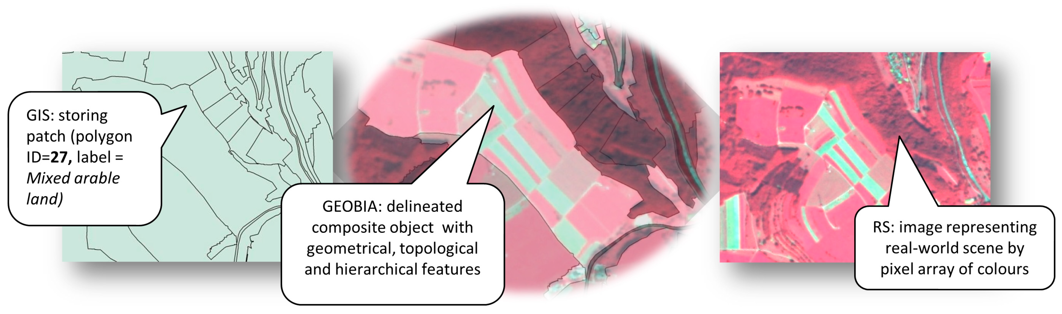
3. GEOBIA: Bridging Remote Sensing and GIS

Geographic information science (GIScience) [50] has emerged as a meta-discipline, serving many application domains in a multidisciplinary manner. In GIScience, the term object-based image analysis (OBIA) was tentatively introduced in 2006 [22,51]. In 2008, it was re-formulated as GEOBIA [9] emphasizing a primary focus on EO data-derived applications and the interdisciplinary integration of (geo-)spatial-temporal reasoning to cope with the massive volume of EO imagery and related information extraction challenges [2]. By 2010, a plethora of published papers focused on the (GE)OBIA approach [52] with increasing more GIScience scholars proposing GEOBIA as a shift in paradigm [8], capable of bridging the semantic information gap from big data in the image-domain, such as EO image time-series (i.e., EO data cubes), to information primitives of the 4D real-world (scene-)domain, to be handled by geographic information systems (GIS).

Imagery as a 2D gridded array of pixels solely stores per-pixel brightness or colour values, but no descriptive content such as object boundaries or semantic information. Instead, any descriptive content needs to be documented in the metadata, detached from the actual sensor data. At present, image content per se cannot be queried, but merely viewed; however attempts towards this vision exist [53]. Similarly, GIS polygon data sets [10] are discrete and finite vector data sets representing discrete categorical or nominal variables rather than numeric variables. Each polygon features a fixed boundary, one identifier, one semantic label, and several spatial and non-spatial attributes. They contain interpreted information or discretized measurements that are statistically aggregated in space. We suggest that the success of GEOBIA as measured by bibliometric measures [8,52] also roots in its mediating power between these two principle data models, which broadly resemble the GIS and RS communities (Figure 4). To prevent image data from being a pure ‘backdrop’ or only serving for orientation, but instead, to turn them into a fully integrated geospatial data source, requires image understanding systems that exploit their contents and contexts at multiple levels.

In particular, image-understanding related to automatically defining the ‘appropriate’ (global) scale(s) to evaluate complex scene components (i.e., image-objects) of varying size, shape, and spatial arrangements still remains a challenge—through progress has been made. For example, the year 2000, saw the public release of eCognition software [34], built upon a semi-automatic image segmentation approach [54] that calculated a global segmentation threshold from local analysis. Hay, Marceau, Dubé, and Buchard [43] also proposed the use of varying sized and shaped spatial filters optimized to the local perceptual image-objects composing a scene; while more recent (open source) multiscale tools also claim an ability to generate both local and global segmentations that are data-driven vs. user driven (though opportunities exist for both) see [55,56,57]. Now, such multiscale segmentation software can be found in many commercial and open source remote sensing and GIS packages.

3.1. Horizontal and Vertical Properties

Conceptually, we may differentiate between two main generic spatial aspects of a real-world scene represented by images: (i) ‘horizontal’ spatial properties of real-world objects at a given spatial scale of analysis, such as size, shape (geometric) properties, and inter-object spatial topological relationships (e.g., inclusion, adjacency) as well as spatial non-topological relationships (e.g., spatial distance, angle measures), and (ii) ‘vertical’ or hierarchical spatial properties and relationships of real-world objects across multiple spatial scales of analysis. From an epistemological viewpoint, the patch model and related concepts within landscape ecology [58,59] offer an intuitive explanation of geographical patterns, depicted on air- or space-borne images. “Patch context matters” [60] (p.47) is another comprehensive statement that highlights the role of space, namely the patch concept in the scene-domain, as a “non-linear portion of a territory, the aspect and/or the substance of which differs from the surrounding environment and which is relatively homogenous” [61] (p.83). Others include (i) the arrangement of patches in terms of their horizontal composition [36,62] and vertical embeddedness [43,63]; (ii) the specific processes attached to them; and (iii) the relevance of describing, measuring, and quantifying both. Though complimentary, it needs to be stated that conceptually there is a difference between the patch concept as described above in the scene-domain, in which homogeneity in function (semantics) or its appearance properties plays a key role, and the patch concept in the image-domain adopted by machine learning-from-data algorithms, in particular CNN.

3.2. Spatial Autocorrelation vs. the Ignorance of Space

Reflectance as a continuous spatially varying phenomenon is represented as a pseudo-continuum within the (regular) grid data model that depending on resolution can be a well-suited approximation of the ‘real-world’. However, whenever we study spatial continua, we seek for gradients, boundaries, regions, and ultimately objects. In other words, we try to translate (pseudo-continuous) geo-fields into (discrete) geo-objects [64] (or vice versa [65]). Regions (or more specifically, image-objects) can be considered as 2D representations of geographic (‘real-world’) objects [66], which are characterised by internal homogeneity and difference to neighbouring regions. How internal homogeneity is defined and which criteria are used to describe it, depends on the complexity and the nature of the objects, as well as the measurements available to be assessed i.e., 5 cm vs. 50 m. In the simplest case, an image region is a set of neighbouring equal intensity pixels, which in the CV literature is sometimes called an aura [67]. In B&W images, or images of high contrast, pixels with equal grey-tones may be readily detected. However, in an 8-bit (or higher) colour image, chances of finding pixels with exactly the same reflectance value are significantly reduced. Homogeneity may then be considered as ‘similarity’ in spectral reflectance, grouping neighbouring pixels of like reflectance. However, it may also extend to textural homogeneity, or even uniformity in pattern or structure. Structural homogeneity may be the most difficult to automate, as it includes ramps, or irregular, yet self-similar arrangements of sub-objects, or interruptions, occlusions, and other effects being introduced by planar projection—all of which can change over spatio-temporal scales (see for example the road displayed in Figure 1c, interrupted by trees/shadows). Human vision can cope with such irregularities according to the gestalt principles [68], but bottom-up strategies of image segmentation (e.g., region growing algorithms) reach their limitations depending on scene complexity.

To delineate and identify image-objects we utilize a core geographic principle, some refer to as the first law of geography [69]. Spatial autocorrelation, the tendency of neighbouring spatial entities (“things” sensu Tobler) to be similar in value, greatly helps in delineating homogenous units (Figure 2b, or Figure 5b). For the typical high (H-)resolution situation [70] in VHR data, i.e., when target features are well resolved by a series of adjacent pixels, autocorrelation is generally high (Figure 5e, f). According to Strahler’s scene model [71], H-resolution (and its pendant L-resolution) depends on the ontological (and scale) domain of the classes of interest. Recently, with the advent of hyperspatial [72] data from RPAS, platforms, the level-of-detail has greatly increased with smaller and smaller targets being resolvable. Still, in particular in combination with the often-limited spectral capacities of many VHR and RPAS platforms, the spatial association of pixels becomes even more relevant. Image segmentation reduces complexity and allows for an ontologically aware analysis [73], which is sensitive to spatial, in addition to spectral, properties. We observe [43] that for images with high spatial autocorrelation, the complexity is lowered (Figure 5b,d as opposed to Figure 5a,c), and interpretation is facilitated. Segmentation and the related GEOBIA approach ably exploit spatial autocorrelation in H-resolution scenes. For describing scene contents by higher order interpretation elements, such as geometric properties of objects (e.g., shape) or context (e.g., topological relations), geospatial concepts are used, including spatial relationship types [74] such as neighbourhood, distance, and hierarchical organisation (Figure 5a–d). Figure 5c illustrates a case where traditional region-growing segmentation would fail due to the heterogeneity of the composed object. In such cases, class modelling has been suggested [36] as a strategy to cope with complex composite classes [62,75], and to use object relationships to build such arrangements based on (heterogeneous, but functionally matching) building blocks.

3.3. From Image to Information Infrastrucuture

The primary aim of collecting EO imagery, from any sensor system is to extract image information and turn scene content into knowledge in a 4D Earth space-time domain. This is done implicitly in our daily visual experiences, but explicitly in scientific geo-applications, by converting scene content into geographical units with nominal (categorical) labels, (typically) stored in vector-based geospatial representations, usually as polygons representing areal features. Whether as a pre-attentive life function, or trained professionally, vision plays a key role as a synonym of scene-from-image reconstruction and understanding. As previously noted, the fact that in vision, spatial information typically dominates colour information [28] (see Figure 1), was—and still is—the foundation of GEOBIA as an alternative paradigm to traditional pixel-based image analysis. In CV (see Section 2.1), spatial concepts in the scene- and image-domain, such as local shape, texture, inter-object spatial topological and spatial non-topological relationships, have been investigated since the late 1970s [76].

Another aspect of the information extraction workflow is interoperability [77]. Ideally, EO data are fully integrated in existing spatial data infrastructures (SDI), and not just as independent image layers, but rather used to automatically update and/or validate existing geospatial information. Using polygon layers from an SDI (e.g., digital cadastre, landscape units, agricultural field boundaries, etc.) can be used to constrain segmentation results, as predefined boundaries [78]. Figure 6a,b show the combination of a parcel-based (the cadastre boundary serves as an outline) and a region-based segmentation (inner boundaries based on internal variance). In Figure 6c, an ATKIS (the German Authoritative Topographic-Cartographic Information System) vegetation layer has been compared for updates using a recent Sentinel-2 scene from April 2018. Next to this, arbitrary tessellations can be linked into existing reference grids, such as the European Terrestrial Reference system, which is based on the respective frame (ETRF) in a given resolution, spatially congruent over all European member states. Figure 6d–f show how the ETRS grid can be used while generating a gridded scene classification map, e.g., for phenological comparative studies (6d), or applying superpixel segmentation [79] which is conditioned by a well-defined set of seed points [80] (Figure 6e).

4. Outlook: GEOBIA Opportunities in the Era of Big Earth Data

In the previous sections—in particular Section 1.1, Section 2.1, Section 2.3 and Section 3—we discussed a number of the broad characteristics of spatial image analysis, none of which are meant as a complete inventory of existing problems, nor as a recipe to any single open problem, but rather as an account of the type of questions we attempt to tackle with spatial image analysis. To improve the productivity of existing GEOBIA systems [82], we draw on recent achievements from neighbouring disciplines, but also tackle open issues of concern to the GEOBIA community based on our combined experience as pioneers in this field. In the following condensed form, we highlight key aspects in multi-source EO image analysis [21], which by examples, provide technology development opportunities to synergistically support GEOBIA, CV, and big EO data analysis.

▪

EO image enhancement: The harmonization of image data values is required at the radiometric and semantic levels of analysis. For example, ESA defines as EO Level 2 information product a single-date multi-spectral (MS) image corrected for atmospheric, adjacency and topographic effects, stacked with its data-derived scene classification map (SCM), whose legend includes quality layers, cloud, and cloud-shadow [83]. Thus far, except for an initial Level-2A pilot production for Sentinel-2 imagery, EO Level 2 products have not been systematically generated at the ground level (i.e., from the image distributor).

▪

EO image storage/analytics: EO big raster data storage and analytics are affected by ongoing limitations to tackle spatio-temporal information in vector format. Novel database management systems (i.e., data cubes), adopted from data warehouse technologies, allow for a more efficient storage and querying of multi-temporal data stacks and time series. By comparison, typical EO data cubes store data in a multi-dimensional data array with two or three spatial dimensions and one non-spatial dimension [84]. The data cube model, for example implemented by the Open Data Cube (ODC) Initiative or the EarthServer project using the (commercial) Rasdaman array database system [85], allows for new data retrieval and management solutions.

▪

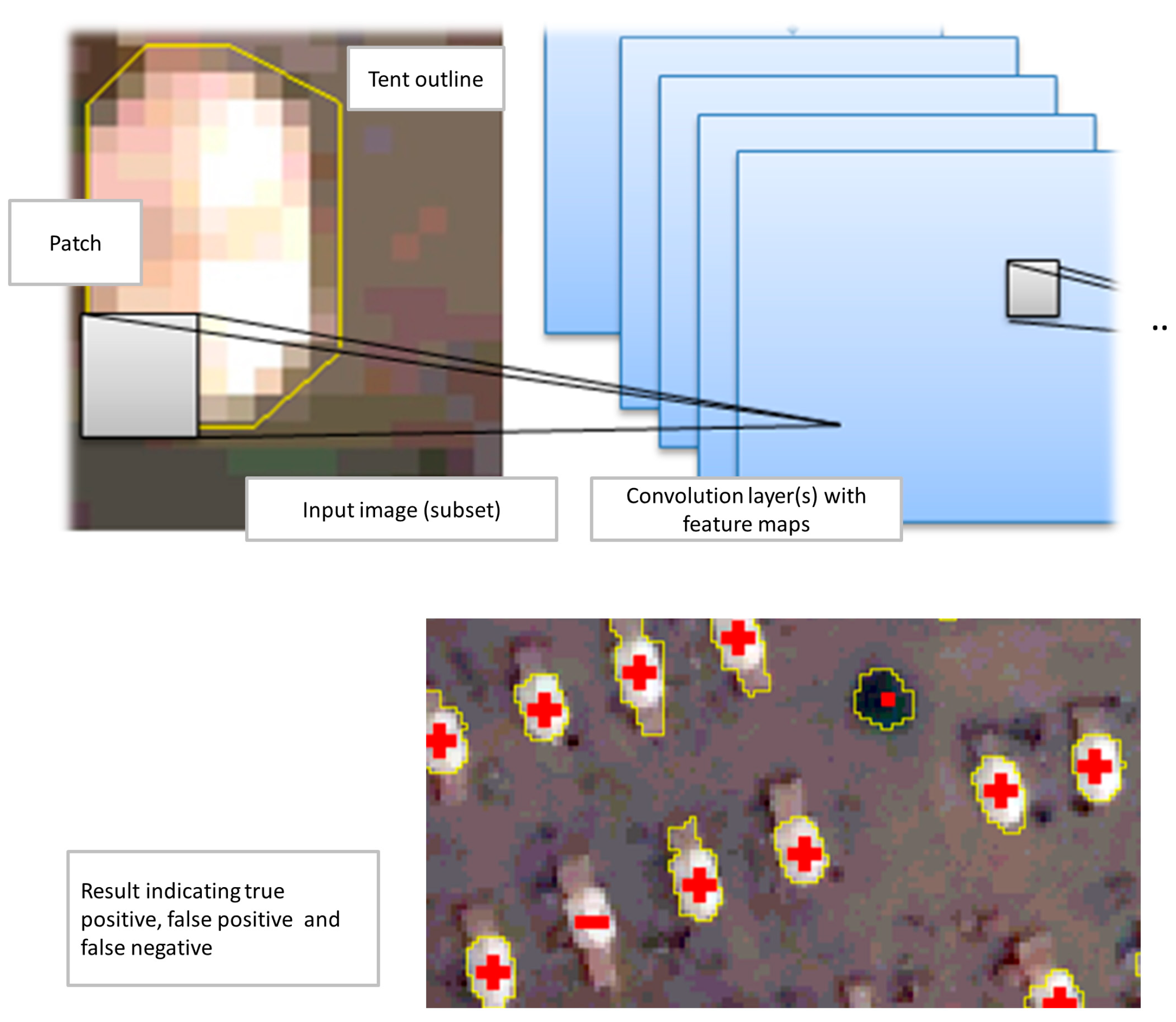
Deep CV systems: To overcome existing limitations, deep (multi-scale) distributed CV systems (i.e., CNNs) are required that allow 2D topology-preserving and context-sensitive image-feature mapping with feedback loops, as an alternative to feedforward 1D image analysis, either pixel- or local window-based.

▪

Hybrid inference: Hybrid (i.e., combined deductive/top-down and inductive/bottom-up) inference is poised to fully exploit scene content. All biological cognitive systems are hybrid inference systems where inductive/bottom-up/phenotypic learning-from-example mechanisms explore the neighbourhood of deductive/top-down/genotypic initial conditions in a solution space. On the contrary, inductive inference currently dominates CV solutions, such as CNNs where a priori knowledge is encoded by a static design.

▪

Convergence of evidence: Structured CV system-of-systems design needs to be implemented based on a convergence of spatial and colour evidence. The well-known engineering principles of modularity, regularity, and hierarchy, typical of scalable systems [48] in agreement with the popular divide-and-conquer problem solving principle [86], are not satisfied by the relative opacity of ‘black box’ artificial neural networks (ANNs)—including CNNs.

▪

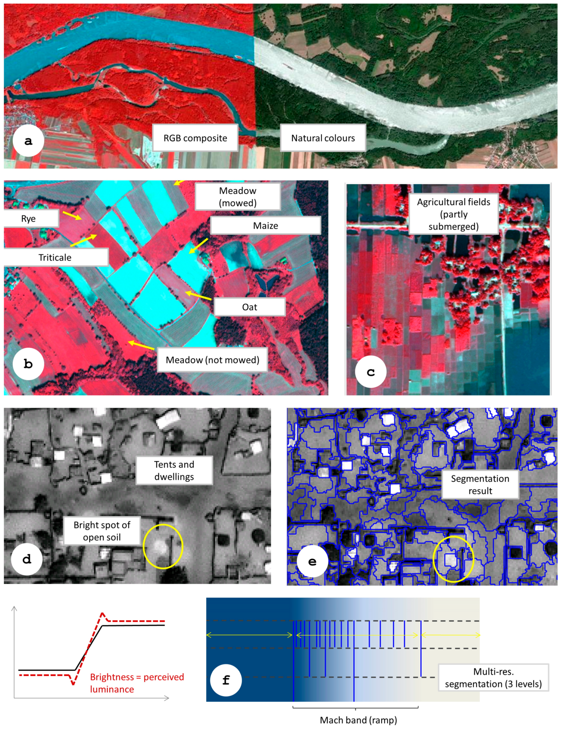
Consistency with human perception: CV (including GEOBIA) needs to be fully consistent with human visual perception. This applies to the issue of perceived (conceptual) boundaries [2] along a gradient of changing patterns according to the principles of Gestalt theory [68], and extends, when benchmarking a CV system on (human) perceptual effects, such as the well-known Mach bands illusion where bright and dark bands are seen at small ramp edges.

▪

Semantic content-based image retrieval (SCBIR): Semantic enrichments of databases or data cubes needed to extend and enhance the current search and query capabilities of large data archives, by content rather than (global) image statistics, e.g., “find all Sentinel-2 scenes, cloud free over flooded areas in the past three years” [87]. While text-based image retrieval is supported by CBIR prototypes, no SCBIR system currently exists in operational mode. Known as query by image content (QBIC) [88], prototypical implementations of CBIR systems take an image, image-object or multi-object examples as query and return from the image database a ranked set of images similar in content to the query. CBIR system prototypes support no semantic querying because they lack CV capabilities in operating mode. A necessary but not sufficient pre-condition to SCBIR is image understanding in operating mode; which is currently still just a concept.

5. Conclusions

In the two decades since its initial development, GEOBIA has reached across many applications, and is a basis for transferring concepts and ideas. In this paper, we have reviewed significant GEOBIA contributions to the EO and the wider AI community and summarized a number of technology development opportunities which if implemented, could synergistically support operational big EO data analysis. GEOBIA concepts are generally ready to be integrated in larger AI solutions manifested in EO cloud processing environments, such as the European Copernicus DIAS (Data and Information Access Service). An operational AI4EO system, in particular for big EO data, cannot neglect spatial concepts, and in order to have the latter fully exploited in operating mode, GEOBIA has to become an integral part of AI; the GEOBIA 2020 conference will explicitly focus on this endeavour. We may argue that whenever greater tasks need to be taken over by AI, then knowledge-based solutions based spatio-temporal properties may be a small, yet critical element in them. For example, the provision of a (low-level) semantic data cube, where for each observation (pixel) at least one nominal (i.e., categorical) interpretation is available and can be queried in the same instance [89] has an enormous potential to be further enriched by spatial concepts. If implemented and upscaled, we may then move from image-specific solutions and case-by-case optimisations of algorithms towards more adaptive learning systems, in other words starting from a “seed AI” [90] and move towards more holistic image-based decision systems. Regardless of how this process evolves, we suggest that the integration of geographic space will remain an integral component necessary to fully exploit EO content and context.

References

1. European Commission. COM(2016) 705 Final. Space Strategy for Europe; European Commission: Brussels, Belgium, 2016. [Google Scholar]
2. Lang, S. Object-based image analysis for remote sensing applications: Modeling reality—dealing with complexity. In Object-Based Image Analysis—Spatial Concepts for Knowledge-Driven Remote Sensing Applications; Blaschke, T., Lang, S., Hay, G.J., Eds.; Springer: Berlin, Germany, 2008; pp. 3–28. [Google Scholar]
3. Iqbal, Q.; Aggarwal, J.K. Image retrieval via isotropic and anisotropic mappings. Pattern Recognit. 2002, 35, 2673–2686. [Google Scholar] [CrossRef]
4. Murphy, G. Categories and Concepts. In Psychology; Biswas-Diener, R., Diener, E., Eds.; DEF Publishers: Champaign, IL, USA, 2014. [Google Scholar]
5. Lang, S.; Tiede, D. Geospatial data integration in OBIA—implications of accuracy and validity. In Remote Sensing Handbook, Volume I—Land Resources: Monitoring, Modeling, and Mapping; Thenkabail, P., Ed.; Taylor & Francis: New York, NY, USA, 2015; Volume I, pp. 295–316. [Google Scholar]
6. Marr, D. Vision; W.H. Freeman: New York, NY, USA, 1982. [Google Scholar]
7. Tomlin, D.C. GIS and Cartographic Modeling; Prentice Hall: Upper Saddle River, NJ, USA, 1990. [Google Scholar]
8. Blaschke, T.; Hay, G.J.; Kelly, M.; Lang, S.; Hofmann, P.; Addink, E.; Feitosa, R.Q.; Van der Meer, F.; Van der Werff, H.; Van Coillie, F.; et al. Geographic Object-based Image Analysis: A new paradigm in Remote Sensing and Geographic Information Science. J. Photogramm. Remote Sens. 2014, 87, 180–191. [Google Scholar] [CrossRef] [PubMed]
9. Hay, G.J.; Castilla, G. Geographic object-based image analysis (GEOBIA): A new name for a new discipline. In Object-Based Image Analysis: Spatial Concepts for Knowledge-Driven Remote Sensing Applications; Blaschke, T., Lang, S., Hay, G.J., Eds.; Springer: Berlin/Heidelberg, Germany, 2008. [Google Scholar]
10. Open Geospatial Consortium (OGC). OpenGIS® Implementation Standard for Geographic Information—Simple Feature Access—Part 1: Common Architecture. Available online: http://www.opengeospatial.org/standards/is (accessed on 5 May 2019).
11. Hay, G.; Niemann, K.O. Visualizing 3-D Texture: A Three-Dimensional Structural Approach to Model Forest Texture. Can. J. Remote Sens. 1994, 20, 90–101. [Google Scholar]
12. Cian, F.; Marconcini, M.; Ceccato, P. Normalized difference flood Index for rapid flood mapping: Taking advantage of EO big data. Remote Sens. Environ. 2018, 209, 712–730. [Google Scholar] [CrossRef]
13. Camara, G.; Queiroz, G.; Vinhas, L.; Ferreira, K.; Cartaxo, R.; Simoes, R.; Llapa, E.; Assis, L.; Sanchez, A. The e-sensing architecture for big Earth observation data analysis. In Proceedings of the Conference on Big Data from Space (BIDS), Toulouse, France, 28–30 November 2017; pp. 48–51. [Google Scholar]
14. Blaschke, T.; Lang, S.; Lorup, E.; Strobl, J.; Zeil, P. Object-oriented image processing in an integrated GIS/remote sensing environment and perspectives for environmental applications. Environ. Inf. Plan. Politics Public 2000, 2, 555–570. [Google Scholar]
15. Wulder, M.A.; Coops, N.C. Make Earth observations open access: Freely available satellite imagery will improve science and environmental-monitoring products. Nature 2014, 513, 30. [Google Scholar] [CrossRef]
16. Zeil, P.; Ourevitch, S.; Debien, A.; Pico, U. The Copernicus User Uptake—Copernicus Relays and Copernicus Academy. GI Forum J. Geogr. Inf. Sci. 2017, 253–259. [Google Scholar] [CrossRef]
17. GEO. The Global Earth Observation System of Systems (GEOSS) 10-Year Implementation Plan, Adopted 16 February 2005; GEO: Brussels, Belgium, 2005. [Google Scholar]
18. GEO-CEOS. A Quality Assurance Framework for Earth Observation, Version 4.0 [Group on Earth Observations/Committee on Earth Observation Satellites]; GEO: Brussels, Belgium, 2010. [Google Scholar]
19. Guo, H. Big Earth data. A new frontier in Earth and information science. Big Earth Data 2017, 1, 4–20. [Google Scholar] [CrossRef]
20. Yang, C.; Huang, Q.; Li, Z.; Liu, K.; Hu, F. Big data and cloud computing: Innovation opportunities and challenges. Int. J. Dig. Earth 2017, 10, 13–53. [Google Scholar] [CrossRef]
21. Baraldi, A. Pre-processing, Classification and Semantic Querying of Large-Scale Earth Observation Spaceborne/Airborne/Terrestrial Image Databases: Process and Product Innovations; University of Naples Federico II: Naples, Italy, 2017. [Google Scholar]
22. Lang, S.; Blaschke, T. Bridging remote sensing and GIS–What are the main supportive pillars? Int. Arch. Photogram. Remote Sens. Spat. Inf. Sci. 2006, XXXVIII-4/C42, 4–5. [Google Scholar]
23. Object-Based Image Analysis: Spatial Concepts for Knowledge-Driven Remote Sensing Applications; Blaschke, T.; Lang, S.; Hay, G. (Eds.) Springer: Berlin/Heidelberg, Germany, 2008. [Google Scholar]
24. Hay, G. Visualizing scale-domain manifolds: A multiscale geo-object-based approach. In Scale Issues in Remote Sensing; Weng, Q., Ed.; John Wiley & Sons, Inc.: Hoboken, NJ, USA, 2014. [Google Scholar]
25. Hay, G.; Blaschke, T.; Marceau, D.J.; Bouchard, A. A comparison of three image-object methods for the multiscale analysis of landscape structure. J. Photogramm. Remote Sens. 2003, 1253, 1–19. [Google Scholar] [CrossRef]
26. Capurro, R.; Hjørland, B. The concept of information. In Annual Review of Information Science and Technology; Cronin, B., Ed.; Information Today, Inc.: Medford, NJ, USA, 2003; Volume 37, pp. 343–411. [Google Scholar]
27. Cherkassky, V.F.M. Learning from Data: Concepts, Theory, and Methods; Wiley: Hoboken, NJ, USA, 1998. [Google Scholar]
28. Matsuyama, T.; Hwang, V.S. SIGMA—A Knowledge-Based Aerial Image Understanding System; Plenum Press: New York, NY, USA, 1990. [Google Scholar]
29. Di Gregorio, A.; Jansen, L.J.M. Land Cover Classification System (LCCS): Classification Concepts and User Manual; Food and Agriculture Organization of the United Nations: Rome, Italy, 2005. [Google Scholar]
30. Baraldi, A.; Lang, S.; Tiede, D.; Blaschke, T. Earth observation big data analytics in operating mode for GIScience applications—The (GE)OBIA acronym(s) reconsidered. In Proceedings of the GEOBIA 2018, Montpellier, France, 18–22 June 2018. [Google Scholar]
31. Canny, J. A computational approach to edge detection. IEEE Trans. Pattern Anal. Mach. Intell. 1986, 8, 679–698. [Google Scholar] [CrossRef] [PubMed]
32. Haralick, R.M.; Shapiro, L. Image segmentation techniques. Comput. Graph. Image Process. 1985, 29, 100–132. [Google Scholar] [CrossRef]
33. Horowitz, S.; Pavlidis, T. Picture segmentation by a directed split and merge procedure. In Proceedings of the 2nd International Joint Conference on Pattern Recognition, Prague, Czech Republic, 22–24 November 2019; pp. 424–433. [Google Scholar]
34. Benz, U.; Hofmann, P.; Willhauck, G.; Lingenfelder, I.; Heynen, M. Multi-resolution, object-oriented fuzzy analysis of remote sensing data for GIS-ready information. J. Photogramm. Remote Sens. 2004, 58, 239–258. [Google Scholar] [CrossRef]
35. Pessoa, L. Mach bands: How many models are possible? Recent experimental findings and modeling attempts. Vis. Res. 1996, 36, 3205–3227. [Google Scholar] [CrossRef]
36. Tiede, D.; Lang, S.; Albrecht, F.; Hölbling, D. Object-based class modeling for cadastre constrained delineation of geo-objects. Photogram. Eng. Remote Sens. 2010, 76, 193–202. [Google Scholar] [CrossRef]
37. Principles of Neural Science; Kandel, E.; Schwartz, J.; Jessell, T.M.; Siegelbaum, S.A.; Hudspeth, A.J. (Eds.) Appleton and Lange: Norwalk, CT, USA, 1991; p. 1710. [Google Scholar]
38. Long, J.; Shelhamer, E.; Darrell, T. Fully convolutional networks for semantic segmentation. In Proceedings of the IEEE Conference on Computer Vision and Pattern Recognition, Boston, MA, USA, 7–12 June 2015; pp. 3431–3440. [Google Scholar]
39. Wang, H.; Wang, Y.; Zhang, Q.; Xiang, S.; Pan, C. Gated convolutional neural network for semantic segmentation in high-resolution images. Remote Sens. 2017, 9, 446. [Google Scholar] [CrossRef]
40. Tsotsos, J.K. Analyzing vision at the complexity level. Behav. Brain Sci. 1990, 13, 423–469. [Google Scholar] [CrossRef]
41. Zhu, X.X.; Tuia, D.; Mou, L.; Xia, G.S.; Zhang, L.; Xu, F.; Fraundorfer, F. Deep learning in remote sensing—A review. IEEE Geoscie. Remote Sens. Mag. 2017, 5, 8–36. [Google Scholar] [CrossRef]
42. Blaschke, T.; Strobl, J. What’s wrong with pixels? Some recent developments interfacing remote sensing and GIS. Z. Geoinf. 2001, 14, 12–17. [Google Scholar]
43. Hay, G.J.; Marceau, D.J.; Dubé, P.; Buchard, A. A multiscale framework for landscape analysis: Object-specific analysis and upscaling. Landsc. Ecol. 2001, 16, 471–490. [Google Scholar] [CrossRef]
44. Hay, G.J.; Marceau, D.J. Multiscale Object-Specific Analysis (MOSA): An integrative approach for multiscale landscape analysis. In Remote Sensing and Digital Image Analysis: Including the Spatial Domain; De Jong, S., Van der Meer, F., Eds.; Kluwer Academic Publishers: Dordrecht, The Netherlands, 2004; Volume 5, pp. 71–92. [Google Scholar]
45. Ghorbanzadeh, O.; Tiede, D.; Dabiri, Z.; Sudmanns, M.; Lang, S. Dwelling extraction in refugee camps using CNN—first experiences and lessons learnt. Int. Arch. Photogram. Remote Sens. Spat. Inf. Sci. 2018, XLII, 161–168. [Google Scholar] [CrossRef]
46. LeCun, Y.; Bengio, Y.; Hinton, G. Deep learning. Nature 2015, 521, 435–444. [Google Scholar] [CrossRef] [PubMed]
47. Belgiu, M.; Dragut, L. Random forest in remote sensing: A review of applications and future directions. J. Photogramm. Remote Sens. 2016, 114, 24–31. [Google Scholar] [CrossRef]
48. Lipson, H. Principles of modularity, regularity, and hierarchy for scalable systems. J. Biol. Phys. Chem. 2007, 7, 125–128. [Google Scholar] [CrossRef] [Green Version]
49. Marcus, G. Deep Learning. A Critical Appraisal. arXiv 2018, arXiv:1801.00631. [Google Scholar]
50. Goodchild, M.J. Geographical information science. Int. J. Geogr. Inf. Sci. 1992, 6, 31–45. [Google Scholar] [CrossRef]
51. Blaschke, T.; Lang, S. Object based image analysis for automated information extraction-a synthesis. In Proceedings of the Measuring the Earth II ASPRS Fall Conference, San Antonio, TX, USA, 6–10 November 2006; pp. 6–10. [Google Scholar]
52. Blaschke, T. Object based image analysis for remote sensing. J. Photogramm. Remote Sens. 2010, 65, 2–16. [Google Scholar] [CrossRef] [Green Version]
53. Marshall, W. Proceedings of the The Mission to Create a Searchable Database of Earth’s Surface. Ted Talk. 11 April 2018. Available online: https://archive.org/details/WillMarshall_2018U (accessed on 11 October 2019).
54. Baatz, M.; Schäpe, A. Multiresolution Segmentation: An Optimization Approach for High Quality Multi-Scale Image Segmentation; Strobl, J., Blaschke, T., Griesebner, G., Eds.; Wichmann Verlag: Salzburg, Austria, 2000. [Google Scholar]
55. Grippa, T.; Lennert, M.; Beaumont, B.; Vanhuysse, S.; Stephenne, N.; Wolff, E. An open-source semi-automated processing chain for urban object-based classification. Remote Sens. 2017, 9, 358. [Google Scholar] [CrossRef]
56. Georganos, S.; Grippa, T.; Lennert, M.; Vanhuysse, S.; Johnson, B.A.; Wolff, E. Scale matters: Spatially partitioned unsupervised segmentation parameter optimization for 62 large and heterogeneous satellite images. Remote Sens. 2018, 10, 1440. [Google Scholar] [CrossRef]
57. Momsen, E.; Metz, M. Manual: I.segment. Available online: https://grass.osgeo.org/grass74/manuals/i.segment.html (accessed on 5 May 2019).
58. Wiens, J. Spatial scaling in ecology. Funct. Ecol. 1989, 3, 385–397. [Google Scholar] [CrossRef]
59. Turner, M.; Gardner, R.; O’Neill, R. Landscape Ecology in Theory and Practice. Pattern and Processes; Springer: New York, NY, USA, 2001. [Google Scholar]
60. Wiens, J. The emerging role of patchiness in conservation biology. In The Ecological Basis of Conservation. Heterogeneity, Ecosystems and Biodiversity; Pickett, S., Ostfeld, R.S., Shachak, M., Likens, G.E., Eds.; Springer: New York, NY, USA, 1997; pp. 93–106. [Google Scholar]
61. Forman, R.T.T.; Godron, M. Landscape Ecology; Wiley: New York, NY, USA, 1986. [Google Scholar]
62. Wang, X.; Su, C.; Feng, C.; Zhang, X. Land use mapping based on composite regions in aerial images. Int. J. Remote Sens. 2018, 1–20. [Google Scholar] [CrossRef]
63. Strasser, T.; Lang, S. Object-based class modelling for multi-scale riparian forest habitat mapping. Int. J. Appl. Earth Obs. Geoinf. 2015, 37, 29–37. [Google Scholar] [CrossRef]
64. Goodchild, M.J.; May, Y.; Cova, T.J. Towards a general theory of geographic representation in GIS. Int. J. Geogr. Inf. Sci. 2007, 21, 239–260. [Google Scholar] [CrossRef] [Green Version]
65. Rahman, M.M.; Hay, G.J.; Isabelle, C.; Hemachandaran, B. Transforming image-objects into multiscale fields: A GEOBIA approach to mitigate urban microclimatic variability within h-res thermal infrared airborne flight-lines. Remote Sens. 2014, 6, 9435–9457. [Google Scholar] [CrossRef]
66. Castilla, G.; Hay, G.J. Image-objects and geo-objects. In Object-Based Image Analysis—Spatial Concepts for Knowledge-Driven Remote Sensing Applications; Blaschke, T., Lang, S., Hay, G.J., Eds.; Springer: Berlin/Heidelberg, Germany, 2008; pp. 91–110. [Google Scholar]
67. Snyder, W.E.; Qi, H. Fundamentals of Computer Vision; Cambridge University Press: Cambridge, UK, 2017; p. 390. [Google Scholar]
68. Wertheimer, M. Drei Abhandlungen zur Gestalttheorie; Palm & Enke: Erlangen, Germany, 1925; p. 184. (In German) [Google Scholar]
69. Tobler, W. A computer movie simulating urban growth in the Detroit region. Econ. Geogr. 1970, 46, 234–240. [Google Scholar] [CrossRef]
70. Woodcock, C.E.; Strahler, A.H. The factor of scale in remote sensing. Remote Sens. Environ. 1987, 21, 311–332. [Google Scholar] [CrossRef]
71. Strahler, A.H.; Woodcock, C.E.; Smith, J.A. On the nature of models in remote sensing. Remote Sens. Environ. 1986, 20, 19. [Google Scholar] [CrossRef]
72. Lippitt, C.D. Remote sensing from small unmanned platforms: A paradigm shift. Environ. Pract. 2015, 17, 2. [Google Scholar] [CrossRef]
73. Lippitt, C.D.; Zhang, S. The impact of small unmanned airborne platforms on passive optical remote sensing: A conceptual perspective. Int. J. Remote Sens. 2018, 39, 15. [Google Scholar] [CrossRef]
74. Tiede, D. A new geospatial overlay method for the analysis and visualization of spatial change patterns using object-oriented data modeling concept. Cartogr. Geogr. Inf. Sci. 2014, 41, 227–234. [Google Scholar] [CrossRef] [PubMed]
75. Lang, S.; Kienberger, S.; Tiede, D.; Hagenlocher, M.; Pernkopf, L. Geons—domain-specific regionalization of space. Cartogr. Geogr. Inf. Sci. 2014, 41, 214–226. [Google Scholar] [CrossRef]
76. Nagao, M.; Matsuyama, T. A Structural Analysis of Complex Aerial Photographs; Plenum Press: New York, NY, USA, 1980. [Google Scholar]
77. IEEE. IEEE Standard Computer Dictionary: A Compilation of IEEE Standard Computer Glossaries; IEEE: New York, NY, USA, 1990. [Google Scholar]
78. Griffith, D.; Hay, G.J. Integrating GEOBIA, machine learning, and volunteered geographiciInformation to map vegetation over rooftops. ISPRS Int. J. Geo-Inf. 2018, 7, 462. [Google Scholar] [CrossRef]
79. Achanta, R.; Shaji, A.; Smith, K.; Lucchi, A.; Fua, P.; Süsstrunk, S. SLIC superpixels compared to state-of-the-art superpixel methods. IEEE Trans. Pattern Anal. Mach. Intell. 2012, 34, 2274–2282. [Google Scholar] [CrossRef] [PubMed]
80. Lang, S.; Csillik, O. ETRF grid-constrained superpixels generation in urban areas using multi-sensor very high resolution imagery. GI Forum—J. Geogr. Inf. Sci. 2017, 5, 244–252. [Google Scholar]
81. Baraldi, A. Satellite Image Automatic Mapper™ (SIAM™). A turnkey software button for automatic near-real-time multi-sensor multi-resolution spectral rule-based preliminary classification of spaceborne multi-spectral images. In Recent Patents on Space Technology; NASA Langley Research Center: Hampton, VA, USA, 2011; pp. 81–106. [Google Scholar]
82. Baraldi, A.; Boschetti, L. Operational automatic remote sensing image understanding systems: Beyond Geographic Object-Based and Object-Oriented Image Analysis (GEOBIA/GEOOIA). Part 1: Introduction. Remote Sens. 2012, 4, 2694–2735. [Google Scholar] [CrossRef]
83. Deutsches Zentrum für Luft- und Raumfahrt e.V. (DLR) and VEGA Technologies. Sentinel-2 MSI—Level 2A Products Algorithm Theoretical Basis Document; European Space Agency: Paris, France, 2011. [Google Scholar]
84. Sudmanns, M.; Lang, S.; Tiede, D. Big Earth data: From data to information. GI Forum J. Geog. Inf. Sci. 2018, 2018, 184–193. [Google Scholar] [CrossRef]
85. Baumann, P.; Mazzetti, P.; Ungar, J.; Barbera, R.; Barboni, D.; Beccati, A.; Bigagli, L.; Boldrini, E.; Bruno, R.; Calanducci, A.; et al. Big data analytics for earth sciences. The EarthServer approach. Int. J. Dig. Earth 2016, 1, 3–29. [Google Scholar] [CrossRef]
86. Bishop, C.M. Neural Networks for Pattern Recognition; Clarendon: Oxford, UK, 1995. [Google Scholar]
87. Tiede, D.; Baraldi, A.; Sudmanns, M.; Belgiu, M.; Lang, S. Architecture and prototypical implementation of a semantic querying system for big Earth observation image bases. Eur. J. Remote Sens. 2017, 50, 452–463. [Google Scholar] [CrossRef]
88. Tyagi, V. Content-Based Image Retrieval: Ideas, Influences, and Current Trends; Springer: Singapore, 2017. [Google Scholar]
89. Augustin, H.; Sudmanns, M.; Tiede, D.; Lang, S.; Baraldi, A. Semantic Earth observation data cubes. Data 2019, 4, 102. [Google Scholar] [CrossRef]
90. Bostrom, N. Superintelligence—Paths, Dangers, Strategies; Oxford University Press: Oxford, UK, 2014. [Google Scholar]
Figure 1. Capacities of human vision: (a) WorldView-2 scene of the Danube riparian flood plain near Vienna, Austria showing a continuation of the scene content (from left to right), even if the colour scheme changes from NIR (‘false colour’) to RGB (‘true-colour’); (b) Quickbird image of a rural area in Austria; and (c) Assam, India: agricultural scenes, recognized by field arrangements, while the primary cue is shape and regularity, colour in both cases provides significant additional cues for interpretation. (d) Geoeye-1 panchromatic imagery of a refugee camp in Sudan: brightness helps distinguish tents as small, compact features, while the decisive visual cue is the shadow cast by tents, and when missing (yellow circle), the hypothesis of a white spot representing a tent no longer holds, even if (e) segmented in the same way as others; (f) psychophysical phenomenon of the Mach bands visual illusion—where a luminance (radiance, intensity) ramp meets a plateau, there are spikes of brightness, although there is no discontinuity in the luminance profile; consequently human vision detects two luminance boundaries, one at the beginning and one at the end of the ramp.
Ijgi 08 00474 g001
Figure 2. From 1D to 2D image analysis, a recognizable (pixelated) 2D image (a) of Abraham Lincon (at left) is transformed into the 1D vector data stream shown on the right. This 1D vector data stream, either pixel-based or local window-based, means nothing to a human photointerpreter. This (out-of-context) 1D vector data stream is what the inductive classifier actually ‘sees’ when analysing the (2D) image at left. (b) Similarly, the linear sequence of segmentation and classification—often applied in standard GEOBIA workflows—may suffice for singular feature extraction tasks such as classifying dwellings in a refugee camp, but falls short (c) when modelling ‘composite objects’ such as ecologically relevant complexes, e.g. a mixed-arable land as shown (bottom-right).
Ijgi 08 00474 g002
Figure 3. An image patch with a series of filters for CNN training to extract tents and other dwellings in a refugee camp scene (a); a small subset showing true positives (+), false positive (.), and false negative (-) (b), modified from [45].
Ijgi 08 00474 g003
Figure 4. GEOBIA emerged as a paradigm to mediate between the domain of geospatial entities (in particular, crisp areal features such as those in a vector representation) and continuous field representations, such as those in images.
Ijgi 08 00474 g004
Figure 5. Scene complexity and spatial autocorrelation: two image pairs with different levels of complexity, despite pair-wise similar semantic content, scale and being captured by the same sensor (Worldview-2). (a,b) Two refugee camps in sub-Saharan Africa; two rural landscapes—(c) southern Spain and (d) northern Germany; (e) gradients between homogenous image regions exhibiting high spatial auto-correlation are perceived as boundaries (f) corresponding with the key geographic principle of regionalization.
Ijgi 08 00474 g005
Figure 6. Spatial constraints, SDI integration and information update. (a) Cadastre boundaries mark the outlines of an agricultural property, which consists of several fields, whose boundaries are added by region-based segmentation, (b) outlines are constrained by the digital cadastre. (c) Overlay of ATKIS vegetation layer with recent Sentinel 2 scene from eastern Germany close to the Polish boundary. (d) Scene classification map of a Sentinel-2 image of the Austrian alps (left), as derived by the SIAM® pre-classification software [81], calculated and overlaid on a 100m ETRS grid (right). (e) The Europe-wide ETRS grid (50 m) provides grid spacing centroids for SLICO superpixel generation based on QuickBird imagery of the old town of Salzburg, Austria.
Ijgi 08 00474 g006