A Spatio-Temporal Bayesian Model for Estimating the Effects of Land Use Change on Urban Heat Island


Chongqing Key Laboratory of GIS Application, School of Geography and Tourism, Chongqing Normal University, Chongqing 401331, China
*
Author to whom correspondence should be addressed.
ISPRS Int. J. Geo-Inf. 2019, 8(12), 522; https://0-doi-org.brum.beds.ac.uk/10.3390/ijgi8120522
Submission received: 21 August 2019
/
Revised: 28 October 2019
/
Accepted: 18 November 2019
/
Published: 20 November 2019
Abstract
:The urban heat island (UHI) phenomenon has been identified and studied for over two centuries. As one of the most important factors, land use, in terms of both composition and configuration, strongly influences the UHI. As a result of the availability of detailed data, the modeling of the residual spatio-temporal autocorrelation of UHI, which remains after the land use effects have been removed, becomes possible. In this study, this key statistical problem is tackled by a spatio-temporal Bayesian hierarchical model (BHM). As one of the hottest areas in China, southwest China is chosen as our study area. Results from this study show that the difference of UHI levels between different cities in southwest China becomes large from 2000 to 2015. The variation of the UHI level is dominantly driven by temporal autocorrelation, rather than spatial autocorrelation. Compared with the composition of land use, the configuration has relatively minor influence upon UHI, due to the terrain in the study area. Furthermore, among all land use types, the water body is the most important UHI mitigation factor at the regional scale.
1. Introduction
The process of urbanization has significant impact on the climatic change by influencing the water balance, energy process and air movement [1], which can potentially lead to a warmer thermal climate in urban areas. Previous studies have identified an increasing trend of heat waves, in terms of duration, intensity and frequency, especially in the city [2,3,4]. Most cities in the world show a higher temperature in the city center than in its rural area, which is called the urban heat island (UHI) phenomenon. This phenomenon has caused an increasing number of premature deaths and heat-related diseases [5,6,7]. In addition, the level of energy consumption [8], air quality [9] and biodiversity [10] can also be attributed to the UHI effect.
Studies on UHI investigation started about 200 years ago, when Luke Howard (1772–1864) [11] found that there is a higher temperature in the urban core area than the surrounding rural area of London. Similar studies have been continually conducted. Generally, when calculating the Heat Island Intensity, there are two different ways to distinguish “rural” and “urban” areas: UHI-driven and land-cover driven approaches [4,12]. The former approach separates rural from urban by the temperature pattern, e.g., range and magnitude, while the latter defines the urban and rural areas by different land uses, e.g., urban-green space and urban-rural [4]. Although comparison between the two has been conducted [4,12], the choice of the definition is mainly determined by the data availability and the nature of the study.
Both air temperature and land surface temperature (LST) were used to calculate the UHI: atmospheric UHI and surface UHI, respectively; however, both indicators have specific advantages and disadvantages [12]. LST can normally be measured at a large spatial area from airborne or satellite-borne sensors [13], but it is not a direct measurement of UHI. On the other hand, air temperature directly estimates the UHI, but it is only available at discrete stations through a city. Therefore, although air temperature has more meaning on people’s thermal feeling, it has limitation to calculate the UHI-driven hot island area and land-cover driven micro-urban heat island [12]. Thus, a better knowledge of the continuous distribution of air temperature is crucial, especially to health-related studies.
It has been estimated that air temperature and LST have a significantly positive correlation [12,14]; however, Sheng, Tang, You, Gu and Hu [4] pointed out that these two indicators are not numerically equal, which can lead to the variation of the UHI estimation. Researchers from the urban climate community argued that LST and air temperature should be distinguished, because both the data content and the nature of the data acquisition are different in the two data types [13,15].
UHI tends to increase in terms of both frequency and intensity, due to the joint impact from both the increase of extreme climatic events and the process of climate change [16]. To improve the development of resilient cities, it is necessary to have a better understanding on the relationship between land use and the climatic effects, especially air temperature, to support the decision-making process.
Researchers determined a complex and multi-fold relationship between UHI and the urban environment [17,18]. Jusuf, et al. [19] and Alonso and Renard [20] analyzed the impact of land use change on the variation of UHI using air temperature (meteorological ground measurements) from both the quantitative and qualitative perspective of views. Recently, due to the development of remote sensing technology, land surface temperature (LST) can be easily and widely captured, even at regional and global scales. The temporal resolution of this monitoring can vary from hourly to yearly, depending upon the revisit time frequency. Most previous studies confirmed the positive relationship between LST and the developed built-up area [21], and the negative relationship between LST and vegetation area [22,23,24]. The cooling effect from green spaces is named as the park cool island (PCI) [25,26]. It has been widely accepted that vegetation offers the most important of climatic regulation at different spatial scales [27]. The UHI mitigation effect from any water body has also been widely recognized [28,29,30], although studies on it are not as many as for those to do with green space. However, most studies on water bodies are from a purely spatial context, and a spatio-temporal perspective of view is missing. In addition to the land composition, land configuration, such as the structural characteristics of land use patches and the spatial arrangement, was also determined as an important factor contributing to the UHI [31,32]. However, there is a lack of knowledge concerning the impact of land use change, in terms of both composition and configuration [33], on the variation of UHI at different spatial scales.
A number of analysis methods were applied to estimate this relationship. Examples of studies considering only the spatial context include [31,34,35], while spatial and temporal designs include [21,24,36]. The Pearson’s correlation coefficients and multiple linear regression are two commonly used methods to analyze the covariate effects [37]. However, the UHI contains residual spatio-temporal autocorrelation after the covariate effects have been separated, which disregards the assumption of statistical independence that often substantiates the models [35,38]. The spatial autocorrelation [34,39] and temporal autocorrelation [40] of the UHI pattern were separately discussed by many previous studies. This autocorrelation may be introduced by unmeasured confounding, close neighborhood influence or grouping effects [41]. Therefore, it is important to account for covariant effects and both spatial and temporal structure in one model by including a set of autocorrelated random effects.
This paper pursues two goals: First, to uncover the spatial and temporal autocorrelation of the UHI pattern at regional scale; second, to evaluate the impact of land use change, in terms of both composition and configuration on the spatial and temporal variation of UHI distribution.
2. Study Area, Data and Methods
2.1. Study Area
Southwest China comprises three provinces and one municipality: Sichuan, Guizhou, Yunnan and Chongqing, with latitude and longitude ranging from 21–34° N and 97–110° E, which is one of the most densely populated areas in China [42]. Among them, Sichuan and Chongqing are the top two dense regions, even in their rural areas [43]. Regarding the temperature, the increase trend is more significant in urban area than that in the rural, especially in Yunnan [43]. The three provinces and one municipality comprise 47 cities. The area has complex landform and topography, which includes part of the Tibetan Plateau, the Chengdu Plain, the Sichuan Basin and the Yunnan-Guizhou Plateau [44], which causes unevenly distributed temperature. The average annual temperature is between 14 and 24 °C in most areas, with the highest record 43.5 °C being found in Chongqing in August 2006 [45]. Normally, August is the hottest month, and this, together with the adjacent four months (June, July, September and October), comprises the hot season in Southwest China.
2.2. Data Used
The land use data in 2000, 2005, 2010 and 2015 were developed by Data Center for Resources and Environmental Sciences (DCRES), Chinese Academy of Sciences [46]. Landsat thematic mapper (TM) and enhanced thematic mapper (ETM) data were used as the major sources to derive the land use information through the processes of image fusion, geometric correction, image enhancement, etc. The average classification accuracy is over 0.85. All datasets have the same level one land use classification (farm, water, grassland, forest, barren land and urban land), and have same spatial resolution (~30 m).
The digital elevation model (DEM) used in this study has a spatial resolution of 1 km, which was aggregated from DEM with 90 m resolution. This dataset was captured as the outcome of the Shuttle Radar Topography Mission (SRTM) project in 2000, and the data used in this study was accessed through International Scientific and Technical Data Mirror Site, Computer Network Information Center, Chinese Academy of Sciences [47]. The vertical accuracy requirement for SRTM data is 16 m [48]. The aggregated DEM was applied to the calculation process for solar radiation and air temperature, respectively.
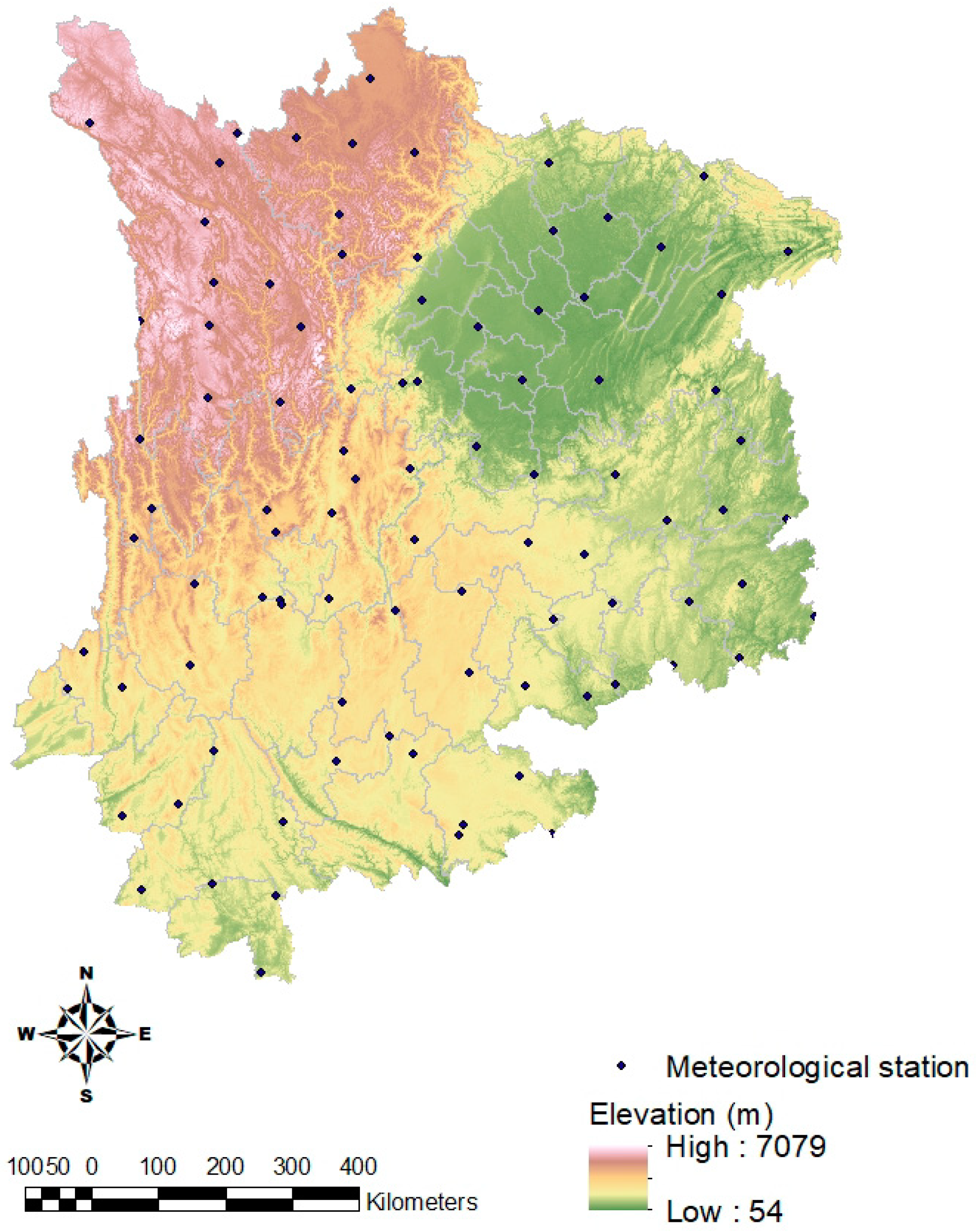
The meteorological data used in this study were collected and managed by the Climate Data Center of the National Meteorological Information Center, China Meteorological Administration [49]. Stations with continuous missing values for over a month were excluded in the analysis. After the filtering process, there are 92 spatially representative stations to monitor air temperature in southwest China (Figure 1). The mean monthly temperature value was interpolated across our whole study area based on the information from these 92 stations, using the method as described in Section 2.3.
2.3. Spatial Interpolation of Air Temperature
Compared with land surface temperature, air temperature is more directly related and important to the biogeochemical processes [50]. Although it can be monitored at discrete locations, there is a need of temperature information for the entire area or specific location. It is possible to interpolate a continuous temperature information using isoline interpolator or expert knowledge; however, Ninyerola, Pons and Roure [50] argued that it is more appropriate to combine a mathematic model and expert knowledge to produce accurate results.
Among all interpolation methods, a multiple regression analysis with Inverse Distance Weighted (IDW) interpolation of the residual errors of ground meteorological information was identified as most accurate method to estimate monthly air temperature with a root-mean-square error (RMSE) of less than 1 °C for all months [50,51]. Specifically, altitude, longitude, latitude and monthly average solar radiation were used as independent variables in the regression, while the residual error was included in the regression to adjust the result, which was interpolated by the IDW method. Therefore, this method was applied in this study to interpolate the four year (2000, 2005, 2010 and 2015) monthly air temperature in southwest China. Altitude is represented by DEM data, and solar radiation was derived from DEM by a solar radiation model [52]. Based on the number of available meteorological stations and the nature of this study, a spatial continuous temperature map with a spatial resolution of 1 km is developed.
2.4. Land Use Mix Indices
Land use mix indices were used in this study to represent the land configuration, which is commonly quantified via the Entropy Index (EI) by many previous studies [53,54]. EI can be traced to the work of Shannon [55,56] to measure the redundancy in data. After the introduction of this index, it has been widely applied in many different research areas outside the information theory, such as communication, ecology, urban planning and land use studies.
The EI can be defined as:
where indicates the percentage of total area of land use i in city j, and represents the total number of land uses in city j. The value of EI ranges from 0 to 1, where 0 stands for homogenous land use, and 1 indicates a prefect mix in a city [53].
2.5. Bayesian Hierarchical Modelling (BHM)
The study region covers 47 cities, which are indexed by . The data was observed for each of these cities for time periods: year 2000, year 2005, year 2010 and year 2015. A spatial and temporal Bayesian hierarchical modeling (BHM) is developed for these data, with inference based on Markov chain Monte Carlo (MCMC) simulation. The first level of this model is as follows:
where , and represent the observed level, expected level and risk of an urban heat island (UHI) in city j during the hot season in year t. is a vector of covariates relating to city j in year t. While stands for the regression parameters. Next, denotes a vector of offsets and represents the random effects for city j and year t, encompassing one or more sets of residual spatio-temporal autocorrelation. This random effect is allowed for any residual spatio-temporal autocorrelation in the observed dataset after the effects are assessed and removed. A number of Gaussian Markov Random Field (GMRF) models were proposed to represent this effect. In this study, this spatio-temporal random autocorrelation was calculated by a model proposed by Napier, et al. [57], and the inference part was developed Markov Chain Monte Carlo (MCMC) in a Bayesian setting. This is because the residual spatial structure cannot be consistent for all time periods. Therefore, the random effect contains two components: an overall temporal trend and a separate spatial structure for each time period, which can be represented by [58]:
where the overall temporal trend is consistent to all areal units, which is interacted with a separate spatial surface at each time period t. These two effects were modeled by the conditional autoregressive (CAR) prior proposed by Leroux, et al. [59]. The latter shares a common spatial dependence value , but a temporally changed parameter . controls the spatial autocorrelation structure, with corresponding for a strong spatial autocorrelation (the intrinsic CAR prior), while represents independent random effects. Similarly, controls the temporal dependence. The set () was designed to examine the magnitude of the spatial variation in the data over time. In the adjacency matrix , stands for the spatial connection between spatial areal units (Sk, Sj). For example, in this study, means that areal units share a common border, and is zero otherwise. Similarly, measures the distance between two time periods.
To estimate the posterior values for the model parameters , different size of samples, ranging from 200 to 1,000,000, were drawn from the posterior distributions using MCMC simulation, based on the Gibbs sampling method and Metropolis-Hastings steps. Both Pearson residual and RMSE were applied to evaluate the performance and fitness of model development.
3. Results and Discussions
3.1. Spatio-Temporal Pattern of UHI
Prior to the estimation of the UHI, air temperature in the hot season (June, July, August, September and October) in 2000, 2005, 2010 and 2015 was interpolated based on the monitoring data at separated stations. Figure 2 gives examples of the interpolated outcomes using the method proposed in this paper. Generally, the temperature distribution shows an unbalanced spatial trend, which decreases from southeast to northwest, with a localized spatio-temporal variation.
In this paper, the UHI was defined by the temperature pattern. Specifically, the range between the highest temperature and lowest temperature across the study area in all five months were calculated as the UHI. This value is different from the overall yearly temperature range, average hot season temperature range and monthly temperature range. Therefore, it takes into account both the heterogeneity and the stratification of spatial and temporal temperature distribution, which balances the local and overall temperature pattern.
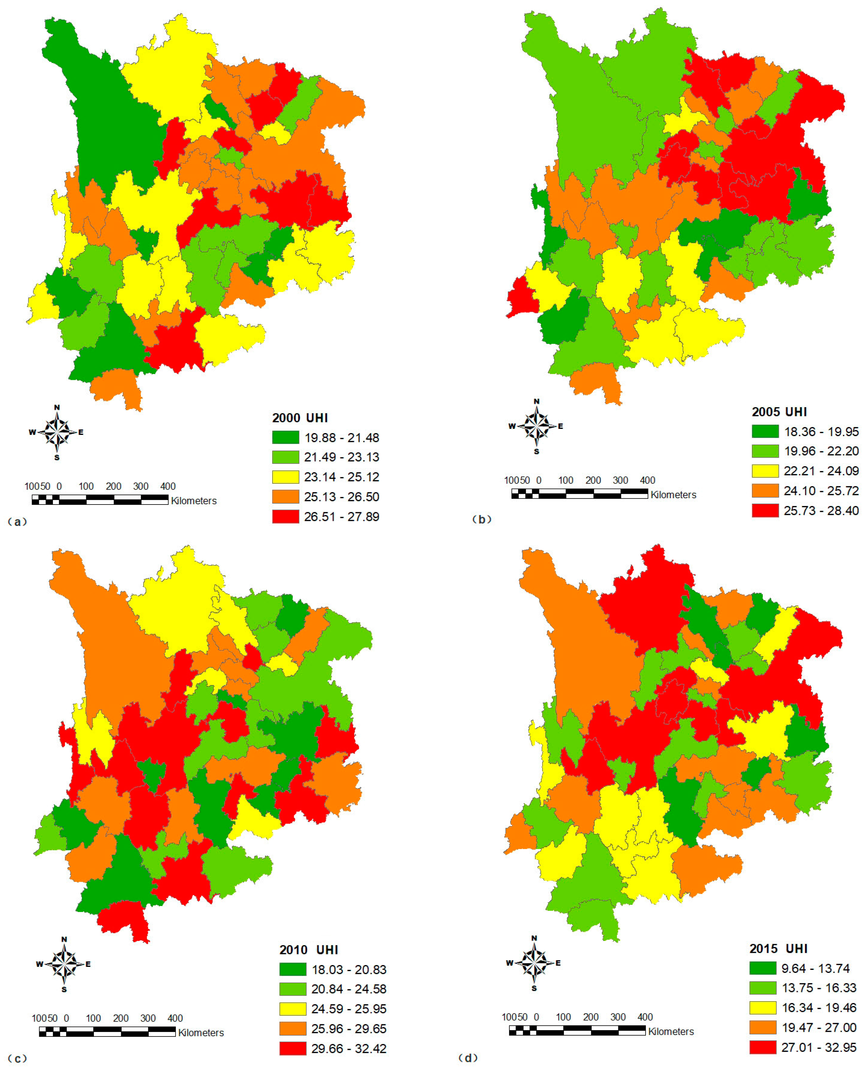
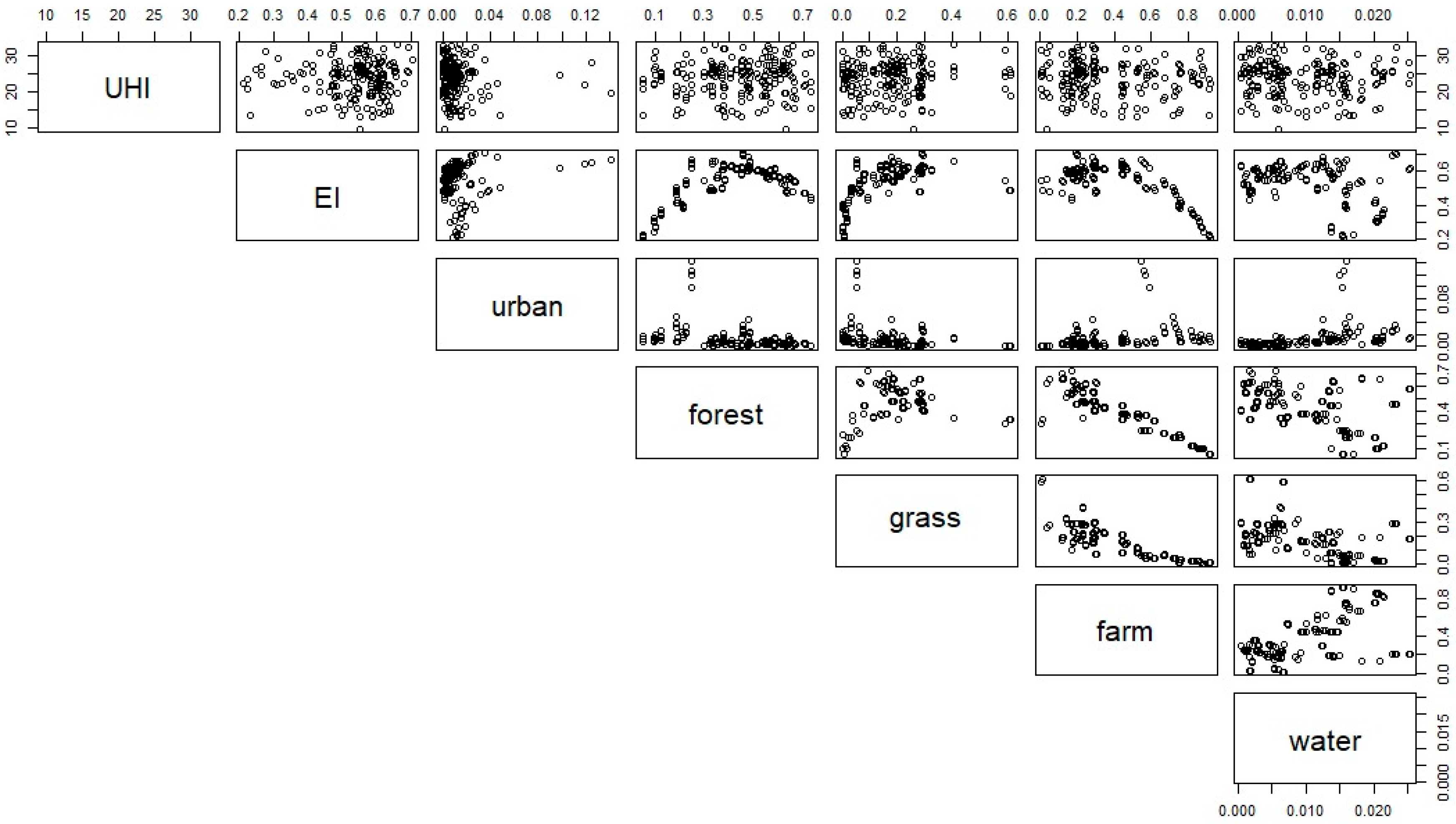
The temperature range in the hot season (five months) of 2000, 2005, 2010 and 2015 in 47 cities was calculated separately (Figure 3). There are two different ways of map presentation, where one is to try to emphasize the temporal variation and the other is to emphasize the spatial variation. This study used Jenks Natural Breaks Classification to optimize the class range for better visual effect and ensure the spatial variation. The level of the UHI increased gradually between 2000 and 2015; however, no clear spatial pattern can be identified. This is because a spatial process normally contains not only the covariate effects, but also spatial or even spatio-temporal autocorrelated random effects, which normally can lead to an incorrect interpretation of the covariate effects. For example, as indicated by Figure 4, no clear correlation pattern can be identified from the scatterplots between UHI and land cover based on the information collected in the 47 cities between 2000 and 2015. This can be partly attributed to the mixed, residual autocorrelated spatio-temporal structure and the covariate effects. Therefore, to accurately estimate the impact of land use change on UHI, the residual autocorrelated spatio-temporal structure needs to be determined first.
3.2. The Land Use Mix
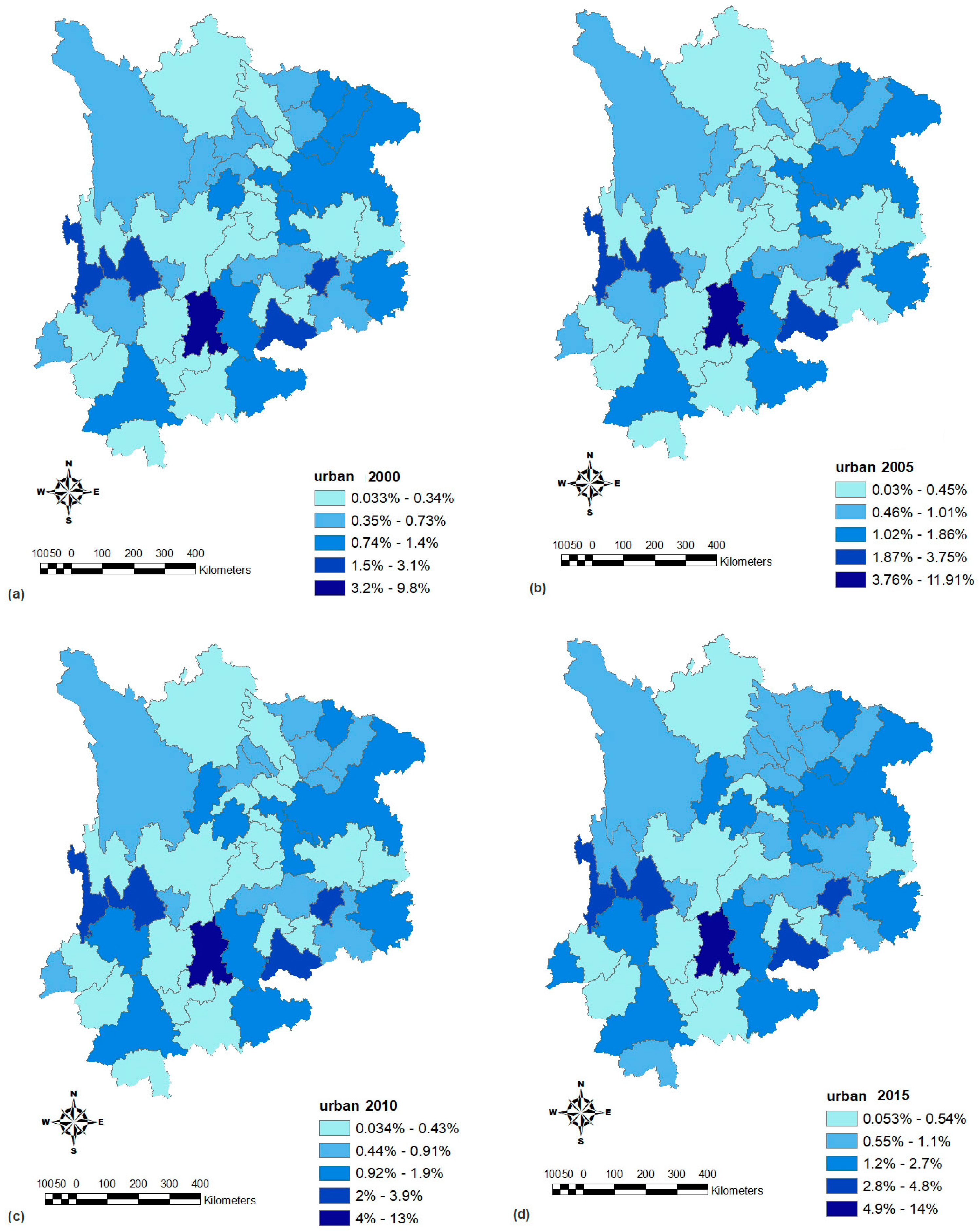
The proportions of different land use (farm, forest, grass, water, urban and others) in each city were calculated for each city in 2000, 2005, 2010 and 2015, separately. Figure 5 demonstrates the example of the urban land variation in 47 cities from 2000 to 2015. Generally, the proportion of urban land use increased in the 15 years, in terms of both the highest level and the lowest level. The overall spatial pattern did not change significantly, and only local variations can be observed.
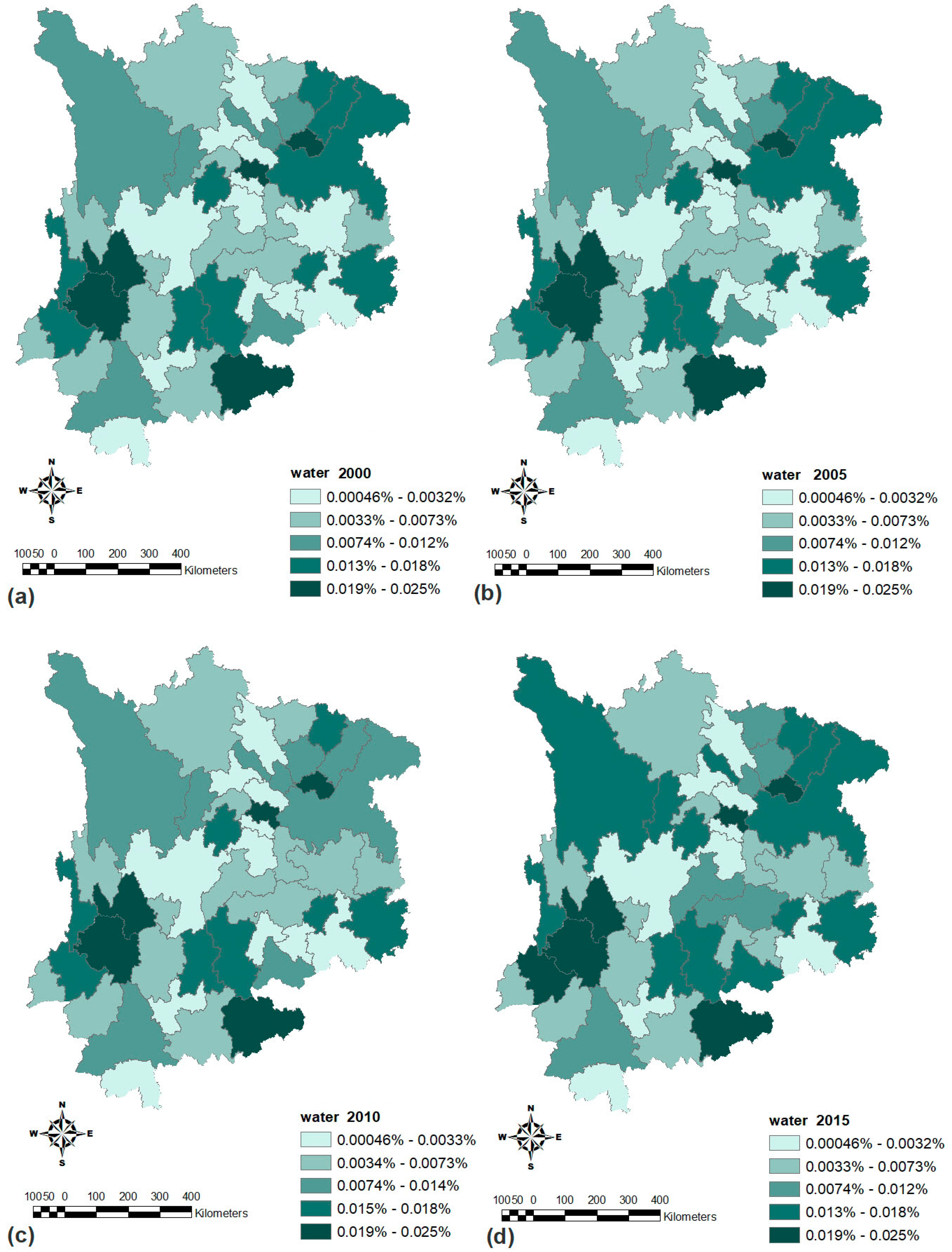
Figure 6 shows the spatio-temporal pattern of water bodies in the study area, which was calculated from the small/big patches (presenting both rivers and lakes) in the land use data, and which was distributed in both in cities or the countryside. The overall proportions did not change significantly between 2000 and 2015, and the largest variation comes from 2015, in which the proportion of water bodies increases in some cities.
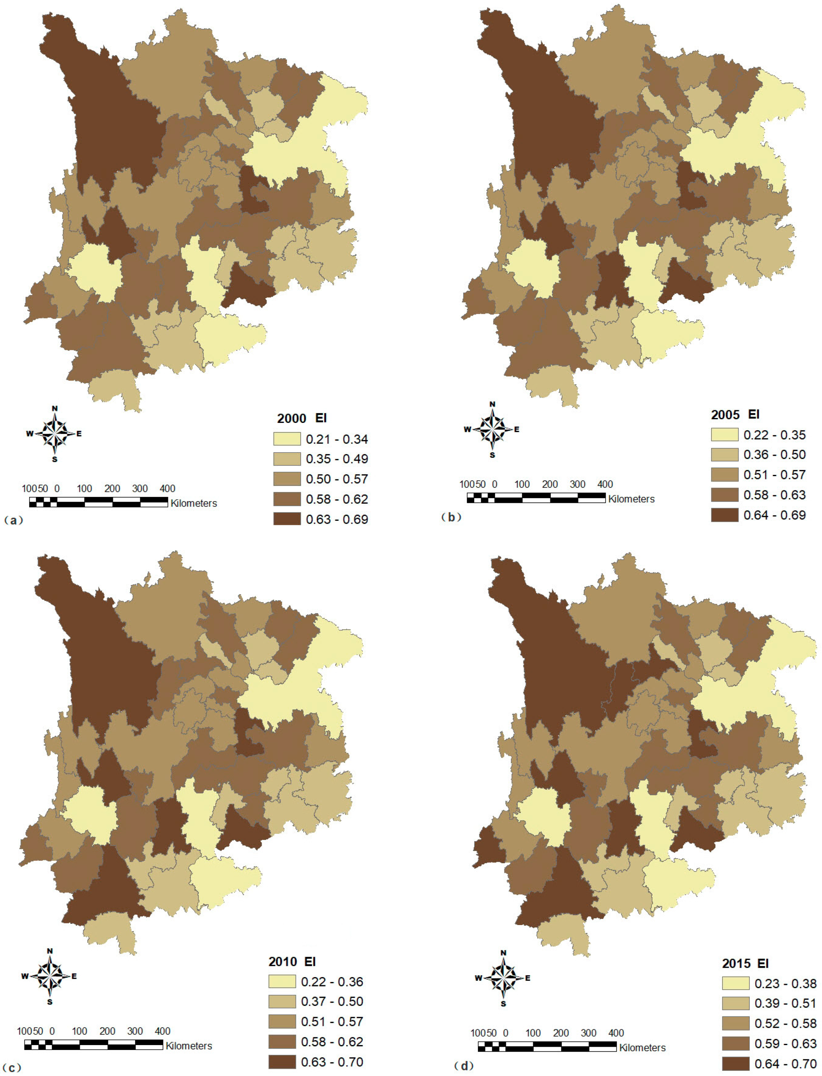
Although the proportion of urban land increased between 2000 and 2015, the level of land use mix did not change correspondingly, as shown in Figure 7. The increase of EI was minor, and only a local variation of land use mix was observed. Therefore, it is necessary to further investigate how much the composition and configuration of land use impacts upon the spatial and temporal variations of the UHI.
3.3. Estimation of Land Use Pattern’s Impact on UHI Distribution
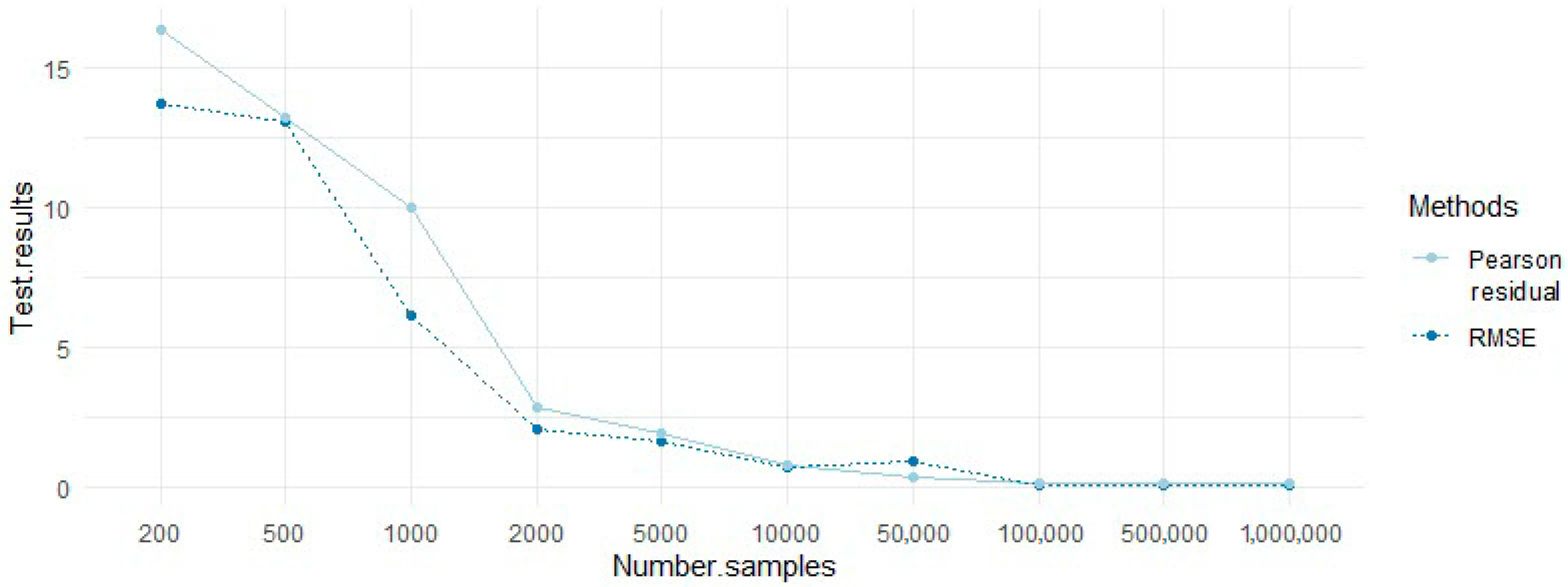
The main aim of this study is to estimate the UHI impacts of different types of land use, and to investigate the strength of spatial and temporal dependences. To ensure the accuracy of the estimation of the posterior values for the model parameters, different sizes of samples were drawn from the posterior distributions using MCMC simulation. Each sample can be viewed as a new simulated dataset. Figure 8 shows that the accuracy of the estimation becomes better as the number of samples increases, in terms of both Pearson residual and RMSE.
The quantified errors are down to near zero, when the number of samples increases to 100,000 and the increase of accuracy is very minor beyond sample size 100,000. Therefore, in this paper, sample size 100,000 was used to estimate the posterior values for the model parameters to balance computing cost and model accuracy.
After the estimation of posterior values, UHI in four different years was fitted based on the Formulas (2) and (3). Figure 9 confirms the accuracy of the model built in this study, as the range and median of ground trues and fitted values are very similar, which gives confidence of the estimation of the parameters we need in this study. This figure also shows that the most serious UHI risk was in 2010, and the overall level of UHI risk decreased in 2015. However, this does not mean that all of the cities experienced low UHI risk in 2015; the UHI levels in different cities distributed sparsely in a very large range in 2015.
The hierarchical model developed in this study purely allows the comparison of spatial autocorrelation and temporal autocorrelation by separating the effects from the covariates. The spatial (rho.S) and temporal (rho.T) dependence parameters exhibit different levels of values in the unit interval (Table 1). Although both spatial and temporal autocorrelation are present in the UHI data, our results suggest that after adjusting for the covariate effects, stronger temporal autocorrelation is present in the UHI data, while spatial autocorrelation is relatively weak in the UHI. In other words, the level of UHI could be more accurately predicted by a time-series analysis, rather than spatial analysis, such as the Kriging method or inverse distance weighting (IDW). This can be partly explained by the terrain in the study area that impedes the application of Tobler’s first law of geography [60].
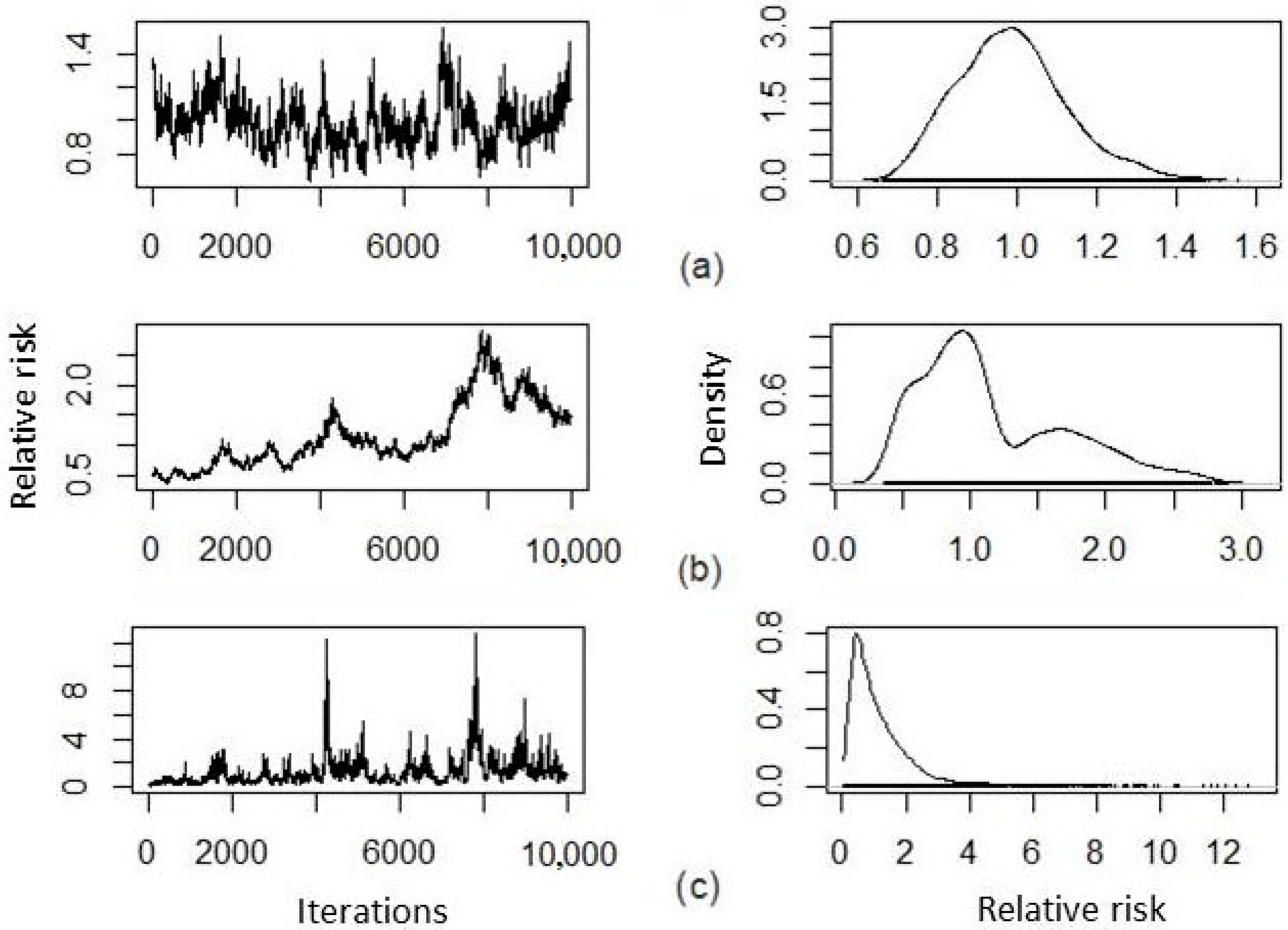
Poisson models are typically presented as relative risks. In this study, the relative risk for a unit increase from a covariate with parameter is presented by the transformation exp(). Therefore, a 5% increased risk can be shown by a relative risk of 1.05. The left side of Figure 10 shows the trace-plots and the right demonstrates the posterior relative risk distributions of a one unit increase for some chosen variables. As demonstrated from the sub-figures, the relative risk from all three different factors shows a different pattern. The trace-plots show that the relative risk from EI is very consistent within a narrow range around one (no impact) during the iteration process, while the relative risk from forest fluctuates significantly, but most values are close to zero, which is also reflected by the density estimates.
As a simplified summary of density estimates, Table 2 shows that five covariates exhibit different relationships with UHI. Different from traditional regression, the impacts from covariates in this study are represented as a posterior median and 95% credible intervals. The table shows that the relative risk of a one percentage increase of urban area is 1.062, suggesting that such an increase corresponds to 6.2% additional UHI risk. While, for one percentage increase in the area of forest, grass and farm, the risk is 0.863, 0.965 and 0.975, respectively, which indicates the mitigation effect of forest on UHI is slightly better than grass and farm. However, as indicated in Table 2, the most significant impact factor is water, which was less compared with other land covers in one study. This study shows at a regional scale, e.g., a group of cities or province, that the size of the water body has an impact on the mitigation of UHI. Although the spatio-temporal variation of water bodies is not significant, its change pattern is very similar as the UHI, especially in 2015. Compared with the composition of land use, the relative risk from the configuration of land use is very minor. The posterior median for the relative risk of a percentage increase in EI is nearly equal to 1, and the 95% credible interval is also very narrow and close to 1 (Figure 10 and Table 2).
There are three points which need to be further explained. First, the comparison of the composition and configuration has been widely discussed and different conclusions were drawn [61,62,63]. This can be attributed to the design of the research and the data used, but most importantly, the inconsistent definition of land configuration is another factor. Second, due to the limitation of data availability, a longer term of analysis should be conducted to evaluate the results of this study. Similarly, different outcomes may be generated in different study areas, due to the variation of geomorphology, climate zones, etc. Finally, the design of the BHM is based upon the assumption of spatial correlation; however, the effect of spatial heterogeneity also exists in the UHI. In the future studies, the combination of the two should be considered in the new designed model.
4. Conclusions
The correlation between land use and UHI has been studied intensively within previous studies. However, due to the limitation of data availability and modeling skill, the residual spatio-temporal autocorrelation of UHI cannot be separated from the covariate effects, which violates the constraint of statistical independence underpinning the correlation models. Therefore, a spatio-temporal BHM model is developed to solve this problem.
The results from this study show that the UHI can be accurately predicted using land use data based on the spatio-temporal BHM model. Different from previous models, the model built in this study can not only estimate the effects of land use on UHI, but also allows for residual spatio-temporal autocorrelation.
The results reveal that an increased proportion of urban area is related to the increased UHI risk, while a decreased proportion of nature environmental space, as measured by both green area and water body, is related to the decreased risks of UHI. Although the mitigation effect of a water body has been discussed before, this study shows that compared with other factors, it is the most significant mitigation factor at the regional scale. Also, compared with the composition of land use, the relative risk from the configuration of land use is much less significant.
One of the key motivations of this study was to separate the residual spatio-temporal autocorrelation from the covariate effects. The outcome from this process shows a stronger temporal autocorrelation in the UHI data, while spatial autocorrelation is relatively weak in the UHI. In other words, the prediction of UHI risk can be more accurate from a temporal dimension. This can be partly explained by the terrain in the study area that is impeding the application of Tobler’s first law of geography. Another finding from this study is that the differentiation of UHI risk in different cities becomes large from 2000 to 2015. The key factors that underpin this trend should be further investigated by future studies.
Author Contributions
Conceptualization, Xin Liu, Zuolin Xiao, Rui Liu; Methodology, Xin Liu, Rui Liu; Formal Analysis, Xin Liu, Zuolin Xiao; Data Curation, Xin Liu, Zuolin Xiao; Writing—Original Draft Preparation, Xin Liu, Zuolin Xiao, Rui Liu; Writing—Review & Editing, Xin Liu, Zuolin Xiao, Rui Liu.
Funding
This research was funded by National Natural Science Foundation of China, grant number 41801063; and Chongqing Postdoctoral Science Fund, grant number XmT2018042.
Acknowledgments
We thank the journal’s editors and anonymous reviewers for their kind comments and valuable suggestions to improve the quality of this paper.
Conflicts of Interest
The authors declare no conflict of interest.
References
- Richards, K.; Oke, T.R. Validation and results of a scale model of dew deposition in urban environments. Int. J. Climatol. 2002, 22, 1915–1933. [Google Scholar] [CrossRef]
- Meehl, G.A.; Tebaldi, C. More intense, more frequent, and longer lasting heat waves in the 21st century. Science 2004, 305, 994–997. [Google Scholar] [CrossRef] [PubMed]
- Isoard, S.; Winograd, M. Adaptation in Europe: Addressing Risks and Opportunities from Climate Change in the Context of Socio-Economic Developments; European Environment Agency (EEA): Luxembourg, 2013; p. 136. [Google Scholar]
- Sheng, L.; Tang, X.; You, H.; Gu, Q.; Hu, H. Comparison of the urban heat island intensity quantified by using air temperature and Landsat land surface temperature in Hangzhou, China. Ecol. Indic. 2017, 72, 738–746. [Google Scholar] [CrossRef]
- Basu, R.; Samet, J.M. Relation between elevated ambient temperature and mortality: A review of the epidemiologic evidence. Epidemiol. Rev. 2002, 24, 190–202. [Google Scholar] [CrossRef] [PubMed]
- Doyon, B.; Bélanger, D.; Gosselin, P. The potential impact of climate change on annual and seasonal mortality for three cities in Quebec, Canada. Int. J. Health Geogr. 2008, 7, 23. [Google Scholar] [CrossRef] [PubMed]
- Méndez-Lázaro, P.A.; Pérez-Cardona, C.M.; Rodríguez, E.; Martínez, O.; Taboas, M.; Bocanegra, A.; Méndez-Tejeda, R. Climate change, heat, and mortality in the tropical urban area of San Juan, Puerto Rico. Int. J. Biometeorol. 2018, 62, 699–707. [Google Scholar] [CrossRef]
- Lowe, S.A. An energy and mortality impact assessment of the urban heat island in the US. Environ. Impact Assess. Rev. 2016, 56, 139–144. [Google Scholar] [CrossRef]
- Grimm, N.B.; Faeth, S.H.; Golubiewski, N.E.; Redman, C.L.; Wu, J.; Bai, X.; Briggs, J.M. Global change and the ecology of cities. Science 2008, 319, 756–760. [Google Scholar] [CrossRef]
- Li, X.-X.; Norford, L.K. Evaluation of cool roof and vegetations in mitigating urban heat island in a tropical city, Singapore. Urban Clim. 2016, 16, 59–74. [Google Scholar] [CrossRef]
- Howard, L. The Climate of London: Deduced from Meteorological Observations, Made at Different Places in the Neighbourhood of the Metropolis; Phillips, W: Lodon, UK, 1818. [Google Scholar]
- Schwarz, N.; Schlink, U.; Franck, U.; Großmann, K. Relationship of land surface and air temperatures and its implications for quantifying urban heat island indicators—An application for the city of Leipzig (Germany). Ecol. Indic. 2012, 18, 693–704. [Google Scholar] [CrossRef]
- Voogt, J.A.; Oke, T.R. Thermal remote sensing of urban climates. Remote Sens. Environ. 2003, 86, 370–384. [Google Scholar] [CrossRef]
- Chen, X.; Su, Y.; Li, D.; Huang, G.; Chen, W.; Chen, S. Study on the cooling effects of urban parks on surrounding environments using Landsat TM data: A case study in Guangzhou, southern China. Int. J. Remote Sens. 2012, 33, 5889–5914. [Google Scholar] [CrossRef]
- Arnfield, A.J. Two decades of urban climate research: A review of turbulence, exchanges of energy and water, and the urban heat island. Int. J. Climatol. 2003, 23, 1–26. [Google Scholar] [CrossRef]
- Gabriel, K.M.; Endlicher, W.R. Urban and rural mortality rates during heat waves in Berlin and Brandenburg, Germany. Environ. Pollut. 2011, 159, 2044–2050. [Google Scholar] [CrossRef] [PubMed]
- Stone, B.; Vargo, J.; Habeeb, D. Managing climate change in cities: Will climate action plans work? Landsc. Urban Plan. 2012, 107, 263–271. [Google Scholar] [CrossRef]
- Kamal-Chaoui, L.; Robert, A. Competitive Cities and Climate Change; OECD Regional Development Working Paper No 2; OECD Publishing: Paris, France, 2009. [Google Scholar]
- Jusuf, S.K.; Wong, N.H.; Hagen, E.; Anggoro, R.; Hong, Y. The influence of land use on the urban heat island in Singapore. Habitat Int. 2007, 31, 232–242. [Google Scholar] [CrossRef]
- Alonso, L.; Renard, F. Integrating Satellite-Derived Data as Spatial Predictors in Multiple Regression Models to Enhance the Knowledge of Air Temperature Patterns. Urban Sci. 2019, 3, 101. [Google Scholar] [CrossRef]
- Song, B.; Park, K. Analysis of Spatiotemporal Urban Temperature Characteristics by Urban Spatial Patterns in Changwon City, South Korea. Sustainability 2019, 11, 3777. [Google Scholar] [CrossRef]
- Zhang, Y.; Odeh, I.O.; Han, C. Bi-temporal characterization of land surface temperature in relation to impervious surface area, NDVI and NDBI, using a sub-pixel image analysis. Int. J. Appl. Earth Obs. Geoinf. 2009, 11, 256–264. [Google Scholar] [CrossRef]
- Li, J.; Song, C.; Cao, L.; Zhu, F.; Meng, X.; Wu, J. Impacts of landscape structure on surface urban heat islands: A case study of Shanghai, China. Remote Sens. Environ. 2011, 115, 3249–3263. [Google Scholar] [CrossRef]
- Amiri, R.; Weng, Q.; Alimohammadi, A.; Alavipanah, S.K. Spatial–temporal dynamics of land surface temperature in relation to fractional vegetation cover and land use/cover in the Tabriz urban area, Iran. Remote Sens. Environ. 2009, 113, 2606–2617. [Google Scholar] [CrossRef]
- Spronken-Smith, R.; Oke, T. Scale modelling of nocturnal cooling in urban parks. Bound. Layer Meteorol. 1999, 93, 287–312. [Google Scholar] [CrossRef]
- Spronken-Smith, R.; Oke, T. The thermal regime of urban parks in two cities with different summer climates. Int. J. Remote Sens. 1998, 19, 2085–2104. [Google Scholar] [CrossRef]
- Lauf, S.; Haase, D.; Kleinschmit, B. Linkages between ecosystem services provisioning, urban growth and shrinkage–A modeling approach assessing ecosystem service trade-offs. Ecol. Indic. 2014, 42, 73–94. [Google Scholar] [CrossRef]
- Du, H.; Song, X.; Jiang, H.; Kan, Z.; Wang, Z.; Cai, Y. Research on the cooling island effects of water body: A case study of Shanghai, China. Ecol. Indic. 2016, 67, 31–38. [Google Scholar] [CrossRef]
- Steeneveld, G.J.; Koopmans, S.; Heusinkveld, B.G.; Theeuwes, N.E. Refreshing the role of open water surfaces on mitigating the maximum urban heat island effect. Landsc. Urban Plan. 2014, 121, 92–96. [Google Scholar] [CrossRef]
- Sun, R.; Chen, L. How can urban water bodies be designed for climate adaptation? Landsc. Urban Plan. 2012, 105, 27–33. [Google Scholar] [CrossRef]
- Rotem-Mindali, O.; Michael, Y.; Helman, D.; Lensky, I.M. The role of local land-use on the urban heat island effect of Tel Aviv as assessed from satellite remote sensing. Appl. Geogr. 2015, 56, 145–153. [Google Scholar] [CrossRef]
- Li, X.; Li, W.; Middel, A.; Harlan, S.; Brazel, A.; Turner, B. Remote sensing of the surface urban heat island and land architecture in Phoenix, Arizona: Combined effects of land composition and configuration and cadastral–demographic–economic factors. Remote Sens. Environ. 2016, 174, 233–243. [Google Scholar] [CrossRef]
- Gustafson, E.J. Quantifying landscape spatial pattern: What is the state of the art? Ecosystems 1998, 1, 143–156. [Google Scholar] [CrossRef]
- Li, X.; Zhou, W.; Ouyang, Z.; Xu, W.; Zheng, H. Spatial pattern of greenspace affects land surface temperature: Evidence from the heavily urbanized Beijing metropolitan area, China. Landsc. Ecol. 2012, 27, 887–898. [Google Scholar] [CrossRef]
- Chun, B.; Guldmann, J.M. Spatial statistical analysis and simulation of the urban heat island in high-density central cities. Landsc. Urban Plan. 2014, 125, 76–88. [Google Scholar] [CrossRef]
- Dissanayake, D.; Morimoto, T.; Ranagalage, M.; Murayama, Y. Land-Use/Land-Cover Changes and Their Impact on Surface Urban Heat Islands: Case Study of Kandy City, Sri Lanka. Climate 2019, 7, 99. [Google Scholar] [CrossRef] [Green Version]
- Connors, J.P.; Galletti, C.S.; Chow, W.T. Landscape configuration and urban heat island effects: Assessing the relationship between landscape characteristics and land surface temperature in Phoenix, Arizona. Landsc. Ecol. 2013, 28, 271–283. [Google Scholar] [CrossRef]
- Foster, G.; Rahmstorf, S. Global temperature evolution 1979–2010. Environ. Res. Lett. 2011, 6, 044022. [Google Scholar] [CrossRef]
- Li, J.-J.; Wang, X.-R.; Wang, X.-J.; Ma, W.-C.; Zhang, H. Remote sensing evaluation of urban heat island and its spatial pattern of the Shanghai metropolitan area, China. Ecol. Complex. 2009, 6, 413–420. [Google Scholar] [CrossRef]
- Mitchell, B.C.; Chakraborty, J. Urban heat and climate justice: A landscape of thermal inequity in Pinellas County, Florida. Geogr. Rev. 2014, 104, 459–480. [Google Scholar] [CrossRef]
- Rushworth, A.; Lee, D.; Mitchell, R. A spatio-temporal model for estimating the long-term effects of air pollution on respiratory hospital admissions in Greater London. Spat. Spatio Temporal Epidemiol. 2014, 10, 29–38. [Google Scholar] [CrossRef] [Green Version]
- Lin, W.; Wen, C.; Wen, Z.; Gang, H. Drought in Southwest China: A Review. Atmos. Ocean. Sci. Lett. 2015, 8, 339–344. [Google Scholar] [CrossRef]
- Jiangxing, T.G.R.G.Z. Change of Urban Heat Island Intensity and Its Effect on Surface Mean Air Temperature Records in Southwest China. J. Appl. Meteorol. Sci. 2008, 6, 722–730. [Google Scholar]
- Zeng, Z.; Wu, W.; Li, Z.; Zhou, Y.; Guo, Y.; Huang, H. Agricultural Drought Risk Assessment in Southwest China. Water 2019, 11, 1064. [Google Scholar] [CrossRef] [Green Version]
- Qin, N.; Chen, X.; Fu, G.; Zhai, J.; Xue, X. Precipitation and temperature trends for the Southwest China: 1960–2007. Hydrol. Process. 2010, 24, 3733–3744. [Google Scholar] [CrossRef]
- DCRES. Land Use and Land Cover Data. Available online: http://www.resdc.cn (accessed on 15 December 2018).
- CNIC. SRTMDEM 90M. Available online: http://www.gscloud.cn (accessed on 15 December 2018).
- Gorokhovich, Y.; Voustianiouk, A. Accuracy assessment of the processed SRTM-based elevation data by CGIAR using field data from USA and Thailand and its relation to the terrain characteristics. Remote Sens. Environ. 2006, 104, 409–415. [Google Scholar] [CrossRef]
- Ren, G.; Zhou, Y.; Chu, Z.; Zhou, J.; Zhang, A.; Guo, J.; Liu, X. Urbanization Effects on Observed Surface Air Temperature Trends in North China. J. Clim. 2008, 21, 1333–1348. [Google Scholar] [CrossRef] [Green Version]
- Ninyerola, M.; Pons, X.; Roure, J.M. Objective air temperature mapping for the Iberian Peninsula using spatial interpolation and GIS. Int. J. Climatol. 2007, 27, 1231–1242. [Google Scholar] [CrossRef]
- Cristóbal, J.; Ninyerola, M.; Pons, X. Modeling air temperature through a combination of remote sensing and GIS data. J. Geophys. Res. 2008, 113, D13106. [Google Scholar] [CrossRef] [Green Version]
- Pons, X. MiraMon; Geographic Information System and Remote Sensing Software; Centre for Ecological Research and Forestry Applications (CREAF): Barcelona, Spain, 2002. [Google Scholar]
- Manaugh, K.; Kreider, T. What is mixed use? Presenting an interaction method for measuring land use mix. J. Transp. Land Use 2013, 6, 63–72. [Google Scholar] [CrossRef]
- Bordoloi, R.; Mote, A.; Sarkar, P.P.; Mallikarjuna, C. Quantification of Land Use diversity in the context of mixed land use. Procedia Soc. Behav. Sci. 2013, 104, 563–572. [Google Scholar] [CrossRef] [Green Version]
- Preckel, P.V. Least Squares and Entropy: A Penalty Function Perspective. Am. J. Agric. Econ. 2001, 83, 366–377. [Google Scholar] [CrossRef]
- Shannon, C.E. A mathematical theory of communication. Bell Syst. Tech. J. 1948, 27, 379–423. [Google Scholar] [CrossRef] [Green Version]
- Napier, G.; Lee, D.; Robertson, C.; Lawson, A.; Pollock, K.G. A model to estimate the impact of changes in MMR vaccine uptake on inequalities in measles susceptibility in Scotland. Stat. Methods Med. Res. 2016, 25, 1185–1200. [Google Scholar] [CrossRef] [PubMed] [Green Version]
- Lee, D.; Rushworth, A.; Napier, G. Spatio-Temporal Areal Unit Modeling in R with Conditional Autoregressive Priors Using the CARBayesST Package. J. Stat. Softw. 2018, 84, 1–39. [Google Scholar] [CrossRef] [Green Version]
- Leroux, B.G.; Lei, X.; Breslow, N. Estimation of Disease Rates in Small Areas: A new Mixed Model for Spatial Dependence. In Statistical Models in Epidemiology, the Environment and Clinical Trials; Springer: New York, NY, USA, 1999; pp. 179–191. [Google Scholar]
- Miller, H.J. Tobler’s first law and spatial analysis. Ann. Assoc. Am. Geogr. 2004, 94, 284–289. [Google Scholar] [CrossRef]
- Zhou, W.; Huang, G.; Cadenasso, M.L. Does spatial configuration matter? Understanding the effects of land cover pattern on land surface temperature in urban landscapes. Landsc. Urban Plan. 2011, 102, 54–63. [Google Scholar] [CrossRef]
- Du, S.; Xiong, Z.; Wang, Y.-C.; Guo, L. Quantifying the multilevel effects of landscape composition and configuration on land surface temperature. Remote Sens. Environ. 2016, 178, 84–92. [Google Scholar] [CrossRef]
- Lan, Y.; Zhan, Q. How do urban buildings impact summer air temperature? The effects of building configurations in space and time. Build. Environ. 2017, 125, 88–98. [Google Scholar] [CrossRef]
Figure 1.
The location of meteorological stations and terrain in the study area.

Figure 2.
Spatial variation of interpolated air temperature in four months: (a) June 2000; (b) October 2000; (c) June 2015; and (d) October 2015.
Figure 2.
Spatial variation of interpolated air temperature in four months: (a) June 2000; (b) October 2000; (c) June 2015; and (d) October 2015.

Figure 3.
The spatio-temporal variation of urban heat island (UHI) distribution in four different years: (a) 2000; (b) 2005; (c) 2010; and (d) 2015.
Figure 3.
The spatio-temporal variation of urban heat island (UHI) distribution in four different years: (a) 2000; (b) 2005; (c) 2010; and (d) 2015.

Figure 4.
Scatterplots between UHI and land cover.

Figure 5.
The proportion of urban land in different cities in four different years: (a) 2000; (b) 2005; (c) 2010; and (d) 2015.
Figure 5.
The proportion of urban land in different cities in four different years: (a) 2000; (b) 2005; (c) 2010; and (d) 2015.

Figure 6.
The proportion of water bodies in different cities in four different years: (a) 2000; (b) 2005; (c) 2010; and (d) 2015.
Figure 6.
The proportion of water bodies in different cities in four different years: (a) 2000; (b) 2005; (c) 2010; and (d) 2015.

Figure 7.
The variation of land use mix quantified by the Entropy Index (EI) in four different years: (a) 2000; (b) 2005; (c) 2010; and (d) 2015.
Figure 7.
The variation of land use mix quantified by the Entropy Index (EI) in four different years: (a) 2000; (b) 2005; (c) 2010; and (d) 2015.

Figure 8.
Comparison of the estimation accuracy of the posterior values for the model parameters with different sizes of samples.
Figure 8.
Comparison of the estimation accuracy of the posterior values for the model parameters with different sizes of samples.

Figure 9.
Comparison of true values (a) and fitted values (b) of UHI (jittered in the x direction to improve the visual effect) in different years and their median values (bold points).
Figure 9.
Comparison of true values (a) and fitted values (b) of UHI (jittered in the x direction to improve the visual effect) in different years and their median values (bold points).

Figure 10.
Posterior distribution of the selected parameters (a) EI, (b) Urban and (c) Forest; The left panels are trace-plots and the right panels contain density estimates.
Figure 10.
Posterior distribution of the selected parameters (a) EI, (b) Urban and (c) Forest; The left panels are trace-plots and the right panels contain density estimates.


Table 1.
The posterior median and 95% credible interval for the spatial and temporal dependence parameters on the urban heat island (UHI).
Table 1.
The posterior median and 95% credible interval for the spatial and temporal dependence parameters on the urban heat island (UHI).
| Median | 2.5% | 97.5% | |
|---|---|---|---|
| rho.S | 0.0533 | 0.0033 | 0.1754 |
| rho.T | 0.3161 | 0.0150 | 0.8650 |
Table 2.
A summary of the estimated covariate effects on UHI.
| Median | 2.5% | 97.5% | |
|---|---|---|---|
| EI | 0.992 | 0.748 | 1.298 |
| Urban | 1.061 | 0.443 | 2.444 |
| Forest | 0.863 | 0.222 | 3.785 |
| Grass | 0.965 | 0.435 | 2.658 |
| Farm | 0.975 | 0.474 | 2.361 |
| Water | 0.351 | 0.007 | 5.849 |
© 2019 by the authors. Licensee MDPI, Basel, Switzerland. This article is an open access article distributed under the terms and conditions of the Creative Commons Attribution (CC BY) license (http://creativecommons.org/licenses/by/4.0/).
Share and Cite
MDPI and ACS Style
Liu, X.; Xiao, Z.; Liu, R. A Spatio-Temporal Bayesian Model for Estimating the Effects of Land Use Change on Urban Heat Island. ISPRS Int. J. Geo-Inf. 2019, 8, 522. https://0-doi-org.brum.beds.ac.uk/10.3390/ijgi8120522
AMA Style
Liu X, Xiao Z, Liu R. A Spatio-Temporal Bayesian Model for Estimating the Effects of Land Use Change on Urban Heat Island. ISPRS International Journal of Geo-Information. 2019; 8(12):522. https://0-doi-org.brum.beds.ac.uk/10.3390/ijgi8120522
Chicago/Turabian StyleLiu, Xin, Zuolin Xiao, and Rui Liu. 2019. "A Spatio-Temporal Bayesian Model for Estimating the Effects of Land Use Change on Urban Heat Island" ISPRS International Journal of Geo-Information 8, no. 12: 522. https://0-doi-org.brum.beds.ac.uk/10.3390/ijgi8120522
Note that from the first issue of 2016, this journal uses article numbers instead of page numbers. See further details here.