Monitoring the Water Quality of Small Water Bodies Using High-Resolution Remote Sensing Data

Abstract

Remotely sensed data can reinforce the abilities of water resources researchers and decision-makers to monitor water quality more effectively. In the past few decades, remote sensing techniques have been widely used to measure qualitative water quality parameters. However, the use of moderate resolution sensors may not meet the requirements for monitoring small water bodies. Water quality in a small dam was assessed using high-resolution satellite data from RapidEye and in situ measurements collected a few days apart. The satellite carries a five-band multispectral optical imager with a ground sampling distance of 5 m at its nadir and a swath width of 80 km. Several different algorithms were evaluated using Pearson correlation coefficients for electrical conductivity (EC), total dissolved soils (TDS), water transparency, water turbidity, depth, suspended particular matter (SPM), and chlorophyll-a. The results indicate strong correlation between the investigated parameters and RapidEye reflectance, especially in the red and red-edge portion with highest correlation between red-edge band and water turbidity (r² = 0.92). Two of the investigated indices showed good correlation in almost all of the water quality parameters with correlation higher than 0.80. The findings of this study emphasize the use of both high-resolution remote sensing imagery and red-edge portion of the electromagnetic spectrum for monitoring several water quality parameters in small water areas.

1. Introduction

Water quality monitoring in surface water is important, in order to obtain quantitative information on the waters characteristics. A challenge to measuring and monitoring water quality in situ is that it can be prohibitively expensive and time consuming. An alternative method to monitor water quality is by using satellite imagery. In the past few decades, remote sensing techniques and capabilities have been studied for monitoring several water quality parameters. Remote sensing is an effective tool for synoptic soil moisture assessment [1], water and water level monitoring [2], water demand modeling [3], groundwater management, flood mapping [4], and water quality monitoring [5]. Depending on the study area, different satellite sensors have been used for water bodies monitoring. Thus, moderate resolution data from Sentinel-1 has been used for water resource management applications [6], Landsat-8 [7,8], and Sentinel-2 [9,10,11,12] have been used for water bodies extraction and water quality monitoring, MODIS (Moderate Resolution Imaging Spectroradiometer) has been used for water quality assessment [13]. Also, unmanned aerial vehicle (UAV) data have been used for water quality measurements [14]. Landsat data have also been used for assessing detailed water quality parameters, such as suspended sediments, water transparency, chlorophyll-a, and turbidity [15]. Water quality parameters help in decision-making regarding the further use of water based on its quality. However, the use of middle or low spatial resolution data (10–30 m) is not useful in monitoring small lakes, dams or rivers.

The main indicators of water quality are chlorophyll-a, water transparency, turbidity, and suspended particulate matter (SPM) [16]. Chlorophyll-a is a commonly used measure of water quality as eutrophication level. Higher concentrations indicate poor water quality, usually when high algal production is maintained due to high chlorophyll-a and nutrient concentrations. Water transparency can also be used as an indicator of water quality. It is measured with the simple Secchi disk depth. Turbidity is the cloudiness or haziness of the water caused by large numbers of individual particles that are generally invisible to the naked eye. The measurement of turbidity is a key test of water quality. The measurement of total dissolved soils (TDS) is also important as it shows the concentration of dissolved solid particles in the water.

The use of satellite data to monitor water quality parameters has been mainly focused on developing algorithms with band combinations. The remote sensing algorithms for water quality assessment generally involves visible and infrared portion of the electromagnetic spectrum. Thus, turbidity, as one of the most important water quality parameters, has been monitored through remote sensing and several remote sensing studies have quantified the relationship between actual and estimated turbidity from satellite remote sensing data [17,18]. Similar investigations have been made for chlorophyll-a [19], SPM [20], water transparency [21], etc. In order to establish the reliability of the remote sensing data, the results are compared with in situ measurements.

Building on this previous work, this study elaborates on monitoring water quality of small water bodies using high-resolution (5 m spatial resolution) data from RapidEye and implements indices widely used in the literature. However, since there are number of indices, in this study we only used indices that gave significant results or indices that needed clarification about their use. That is the case for one of the indices, that was used in the literature under different names, and was used for both turbidity and chlorophyll-a estimation.

Thus, in this study, we use eight different indices retrieved from high spatial resolution satellite sensors for estimating the correlation between the in situ and estimated water quality parameters: pH, electrical conductivity (EC), TDS, water transparency, water turbidity, depth, SPM, and chlorophyll-a. Specific objectives were: a) to retrieve water quality parameters from RapidEye reflectance, and b) to correlate satellite retrieved parameters with in situ measurements. The paper has been structured as follows: The materials and methods sections provide information about the study area, in situ and laboratory measurements, satellite data, and methodology. In the third part of the paper, the results are presented, followed by detailed discussion and conclusion.

2. Materials and Methods

2.1. Study Area

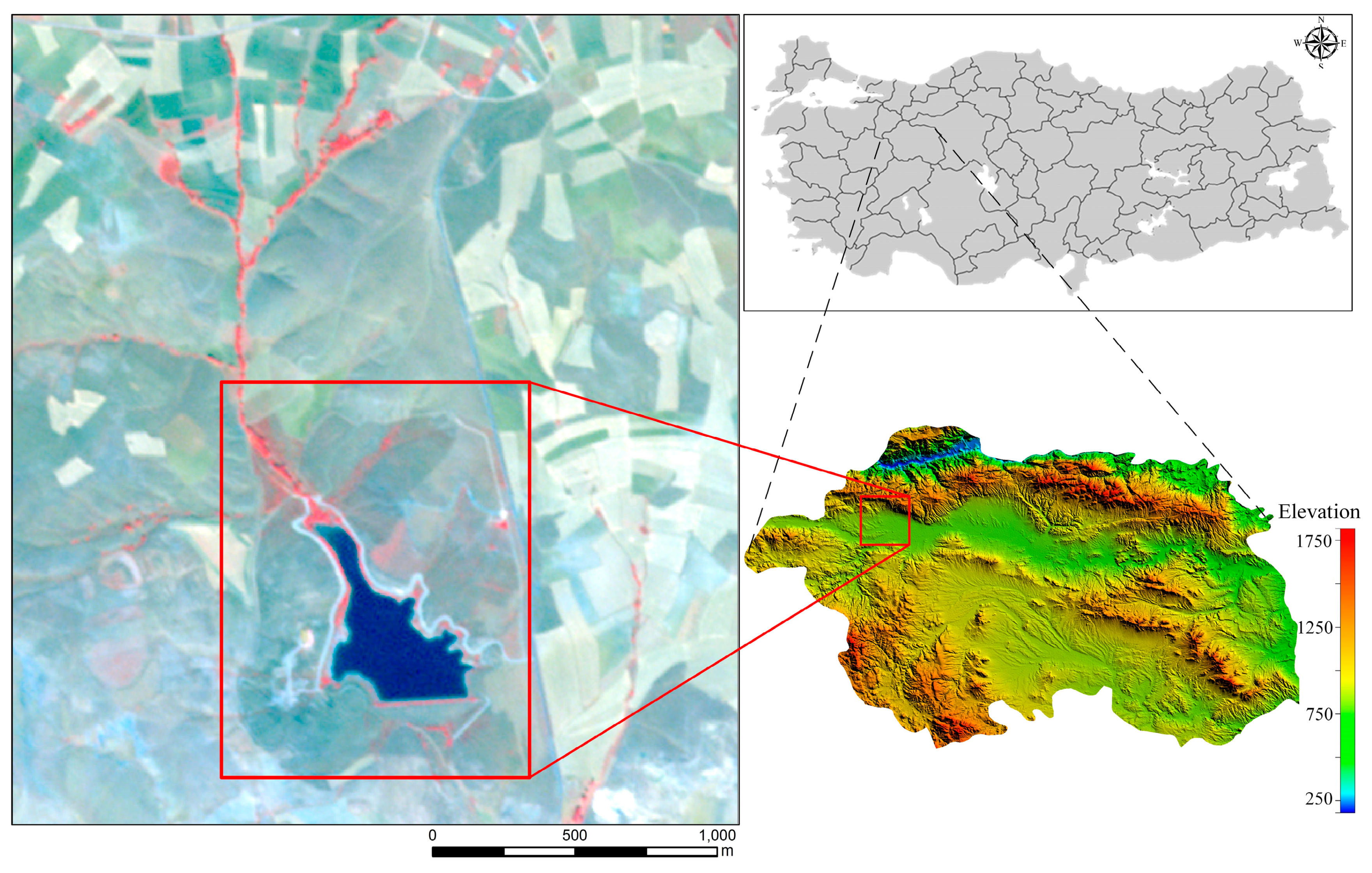
Borabey Dam, built in the period of 1991–1992, is located in Emirce Village on Bozdag slopes north of the Eskisehir city center (Figure 1). The lake covers an area of approximately 166,559 m² at an altitude of approximately 924 m. Borabey Dam was built in order to support the local agriculture. Firstly, the lake was used as the Water Sports Center of Anadolu University in 1999. Later, it was planned to contribute to the drinking and utility water network of Eskisehir. The lake is mainly fed through rain and snow-melting, and one main stream. However, in 2011, this purpose was canceled. Details about Borabey Lake are given in

Table 1. Borabey Dam Technical Information.

Parameter	Length/Area
Barrage Crest Length	411 m
Dam Height	23 m
Fill Volume	368,000 m3
Irrigation Area	248 ha
Storage Volume	1,600,000 m3

[22].

Eskisehir, which is located in the Central Anatolian region, generally has low rainfall. The annual rainfall varies between 300–500 mm. When it comes to the distribution of precipitation according to the seasons, the summer season is generally dry, autumn is rainy, while in spring and winter, there are relatively heavy rains. In winter, a significant proportion of precipitation falls in the form of snow. The climate is continental with very high temperatures during the summer days, but with cool nights, and cold and hard winters.

2.2. In situ and Laboratory Measurements

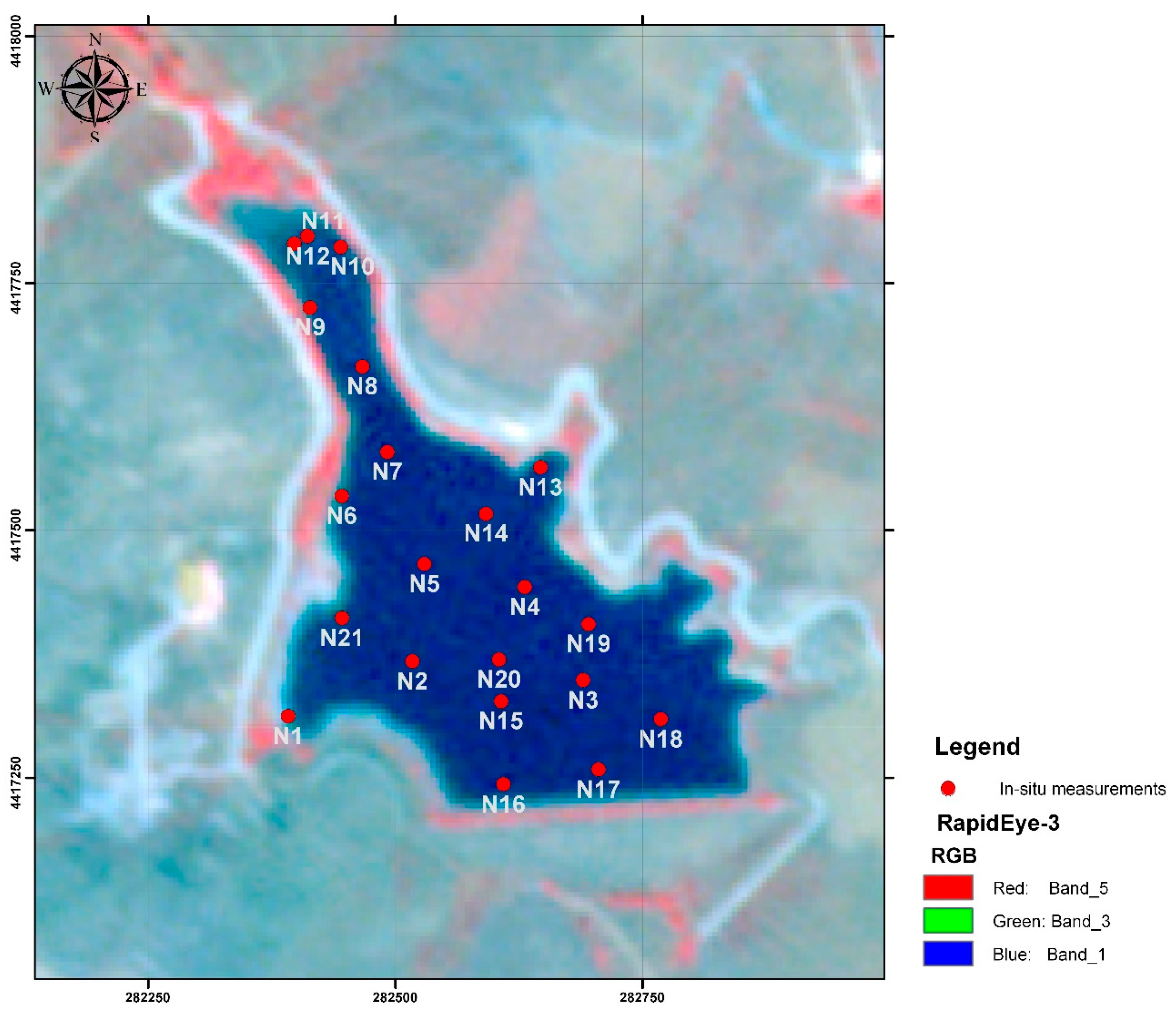
Water sample collections were initiated during the summer season, on August 12, 2014. Following a random sampling technique, water samples were collected and transferred to the laboratory to perform further analyses. In total, twenty-one water samples were collected from the Borabey Lake, and for each sample, the coordinates were recorded with a Global Positioning System (GPS) (Universal Transverse Mercator - UTM coordinates (World Geodetic System – WGS 84) Zone 36S). The samples were collected from the water surface. All of the samples were collected in glass bottles, while the samples used for the Chl-a analyses were transported in opaque bottles. For each sample, the following parameters were estimated: pH; electrical conductivity (EC); total dissolved solids (TDS); Water transparency (Secchi Disk Depth—SDD); depth; turbidity; suspended particulate matter (SPM); and chlorophyll-a (Chl-a). For all of the parameters, two measurements were made and then averaged. Since there was no significant difference between the two readings of the Chl-a, only the average values were given.

pH, EC and TDS values were measured with portable multimeter (Hach HQ40d). Turbidity was measured with a portable field type turbidity meter—(WTW—Turb® 355 IR) as NTU unit. A black/white stripe and 25-cm diameter Secchi disk was used for measuring SDD values. Especially, midday hours are preferred for the measuring SDD values. Chl-a values are measured with using Standard Methods (10200 H) analyzed with a spectrophotometer; SPM values were measured with a gravimetric method at the laboratory. In order to determine the SPM amount, the water samples were filtered through a membrane filter (0.45 µm pore size) and Sartorious filtration apparatus was used.

2.3. Satellite Data

One RapidEye product acquired three days after the in situ measurements, August 17, 2014, was used in this study. The RapidEye instrument acquires data in five different spectral bands (

Table 2. Spectral bands for the RapidEye Satellite Constellation.

Band No	Band Name	Spectral Range [µm]
B1	Blue	440–510
B2	Green	520–590
B3	Red	630–685
B4	Red-Edge	690–730
B5	Near Infra-red	760–850

) with 5 m spatial and approximately six days temporal resolution. The products included a standard geometric correction resampled to a 5 × 5 m pixel size. The data were collected from the Planet Explorer webpage [23]. The RapidEye image with the in situ measurements are given in Figure 2.

2.4. Methods

In situ measurements were used to evaluate eight different remote sensing indices that were successfully used and proposed in the literature for different remote sensing sensors. For simplicity, the indices have been renamed as I1-I8 (

Table 3. List of indices tested in this study.

No	Index (Wavelength)	Index (RapidEye Bands)	Reference
I1	(R560-R805)/(R560+R805)	(B2-B5)/(B2+B5)	[24]
I2	(R560-R710)/(R560+R710)	(B2-B4)/(B2+B4)	[25]
I3	(R660-R560)/(R660+R560)	(B3-B2)/(B3+B2)	[27]
I4	(R710-R660)/(R710+R660)	(B5-B4)/(B5+B4)	[29]
I5	R560/R660	B2/B4	[30]
I6	R660/R710	B4/B5	[33]
I7	R660/R560	B4/B2	[31]
I8	(R660×R560)/R475	(B3×B2)/B1	[32]

). The structure of the first four indices is similar to the widely used Normalized Difference Vegetation Index (NDVI). The first index I1, Normalized Difference Water Index (NDWI) [24], has been widely used for water bodies extraction. Even though the index has been developed to delineate open water features, it is also assumed that it can provide turbidity estimations of water bodies. The index is calculated from the green and near-infrared bands, which are highly sensitive to water contents. I2 is similar to the widely used Normalized Difference Chlorophyll Index (NDCI) [25], but instead of red, uses the red-edge band. I3, or Normalized Difference Turbidity Index NDTI [26,27], uses red and green reflectances for estimating the turbidity in water bodies. However, the same index has been used for chlorophyll-a estimation [25,28,29]. I4 was formed from the red and red-edge portion of the electromagnetic spectrum [29]. I5-I7 are two band ratios, successfully used in the literature for water quality assessment. Namely, the green–red ratio, I5, and the red–red edge ratio have been successfully used for water quality monitoring, especially in chlorophyll-a estimation [30,31]. Similar to I5, I7 is a red–green ratio, used for total suspended matter (TSM) estimation [31]. 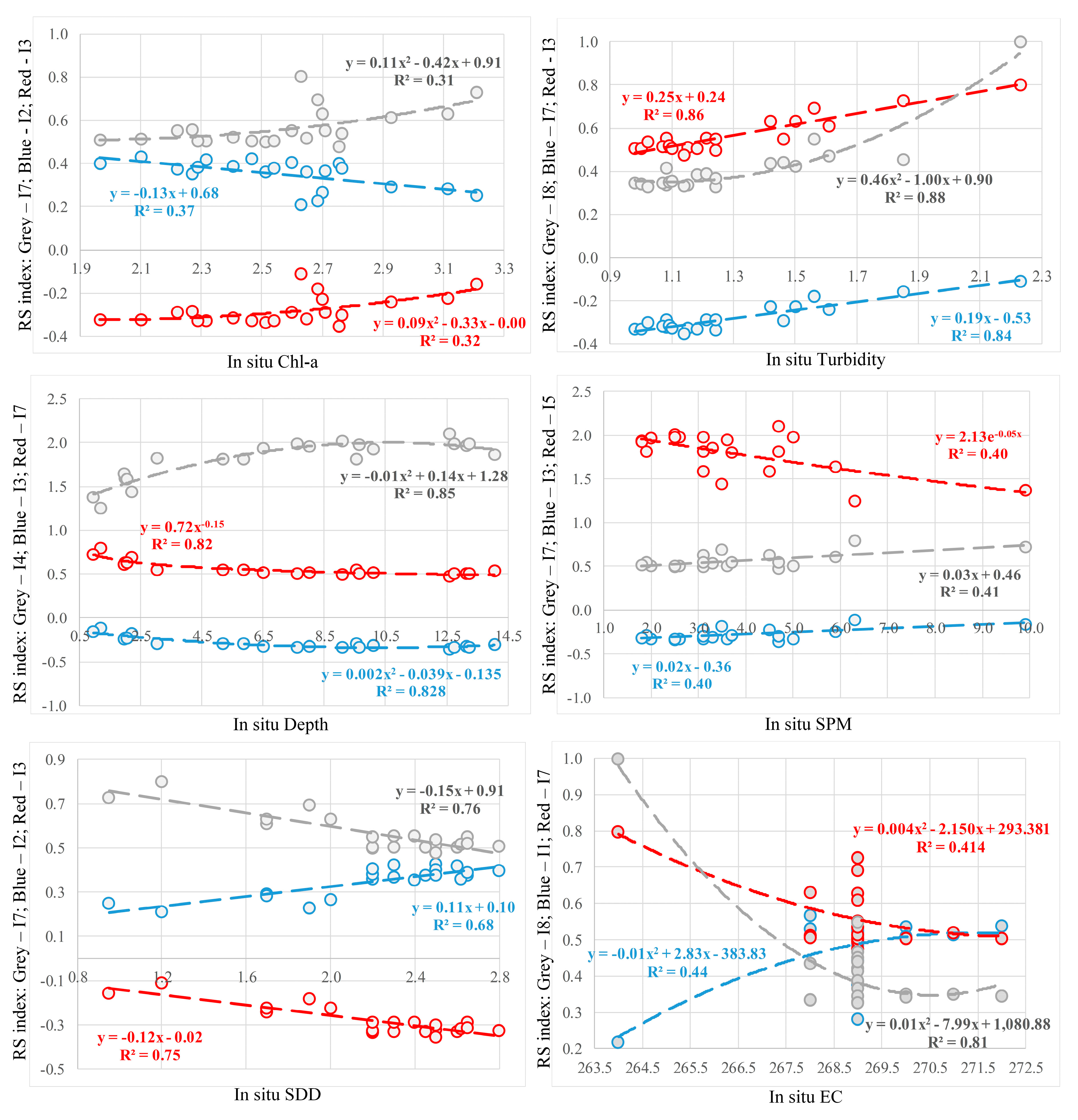I8 is a three-band index used for turbidity estimation [32]. The indices were then adjusted according to the RapidEye satellite sensor bands. Afterward, the results from the retrieved indices were statistically analyzed against the water quality parameters from the in situ and laboratory measurements. In addition, correlation analyses were made between every spectral band from RapidEye and every water quality parameters used in this study, and between the in situ and laboratory measurements of the water quality parameters.

3. Results

3.1. In Situ Data

The results of the in situ and laboratory measurements are summarized in

Table 4. In situ data of the investigated water quality parameters collected on 12 August 2014.

Parameters	Min	Max	Mean
pH	8.42	8.87	8.79
EC (uS/cm)	264.00	272.00	268.95
TDS (mg/L)	125.50	129.80	128.40
SDD_1 (m)	0.95	2.60	2.11
SDD_2 (m)	0.95	2.80	2.21
SDD_avg (m)	0.95	2.70	2.16
Depth (m)	0.95	14.05	7.18
Turbidity _1 (NTU)	0.93	2.23	1.31
Turbidity_2 (NTU)	0.98	2.23	1.30
Turbidity_avg (NTU)	0.96	2.23	1.31
SPM (mg m−3)	1.80	9.90	3.79
Chl-a (mg m−3)	1.97	3.21	2.56

. The minimum, maximum and mean values of the eight studied water quality parameters of all 21 measurements collected on August 12, 2014 are presented. In addition, a polynomial relationship was obtained between in situ measurements of SDD and turbidity (r² = 0.79) and in situ measurements of SDD and laboratory measurement of chlorophyll-a (r² = 0.51). The results are shown in Figure 3.

3.2. RapidEye Data vs. In Situ and Laboratory Data results

In situ and laboratory water quality parameters were collected five days before the satellite image. Band by band correlation was calculated between the RapidEye data and the in situ/laboratory measurements. Also, significance levels for every correlation were calculated. The results are given in

Table 5. Pearson’s correlation coefficient between RapidEye reflectance and in situ and laboratory measurements.

	RapidEye Bands
Parameters	B1_Blue	B2_Green	B3_Red	B4_Red Edge	B5_NIR
EC	−0.77	−0.75	−0.75	−0.72	−0.73
TDS	−0.40	−0.52	−0.45	−0.39	−0.43
SSD_1	−0.56	−0.52	−0.74	−0.75	−0.67
SSD_2	−0.59	−0.52	−0.75	−0.76	−0.68
SSD_Av	−0.58	−0.52	−0.75	−0.75	−0.67
Depth	−0.44	−0.46	−0.65	−0.67	−0.57
Turb_1	0.73	0.68	0.83	0.87	0.81
Turb_2	0.74	0.73	0.89	0.89	0.84
Turb_Av	0.74	0.71	0.86	0.88	0.85
SPM_av	0.41	0.27	0.49	0.45	0.42
Chl-a	0.19	0.11	0.33	0.39	0.29

. The results of pH were not presented, as there was no correlation with the satellite data.

Although high correlations were noticed in the near infra-red (NIR) part, all of the water quality parameters gave highest correlation with the red and red-edge parts of the spectrum. The highest correlation was noticed between the in situ turbidity and the red-edge band with R = 0.9, and p = 0.00. The chlorophyll-a had lowest with R = 0.39 in the red-edge portion. However, after analyzing the results, it was concluded that the first measurement was divergent from the others, thus, after the first measurement was excluded from the statistical analyses, the correlation was R = 0.53, and p = 0.02. The results are shown in Figure 4. For better visualization, normalization of the data was performed (0–1).

The in situ and laboratory measurement values were also regressed against the different band combinations (Table 3) successfully used in the literature for different sensors. The correlations between the indices retrieved from RapidEye data and the in situ and laboratory measurements were calculated. Also, significance levels for every correlation were calculated. The results are given in

Table 6. Correlation (R) RapidEye indices and in situ measurements.

WQ Parameter	I1	I2	I3	I4	I5	I6	I7	I8
EC	0.6	0.5	−0.59	0.14	0.56	0.39	−0.61	−0.76
TDS	0.28	0.16	−0.28	0.28	0.25	0.17	−0.3	−0.49
SDD_1	0.76	0.81	−0.86	0	0.85	0.51	−0.86	−0.68
SDD_2	0.77	0.83	−0.87	−0.02	0.86	0.5	−0.87	−0.68
SDD_av	0.77	0.82	−0.87	−0.01	0.86	0.51	−0.87	−0.68
Depth	0.67	0.76	−0.8	−0.01	0.82	0.31	−0.78	−0.6
Turb_1	−0.85	−0.85	0.92	0.08	−0.86	−0.64	0.87	0.79
Turb_2	−0.87	−0.84	0.92	−0.08	−0.9	−0.6	0.93	0.86
Turb_av	−0.87	−0.84	0.92	0.01	−0.9	−0.64	0.92	0.84
SPM	−0.51	−0.51	0.63	−0.23	−0.62	−0.31	0.64	0.42
Chl-a	−0.48	−0.61	0.54	0.26	−0.55	−0.3	0.53	0.26

and some significant results are shown in Figure 5.

The EC has the highest correlation with the I8 index, index that is generally used for estimating water turbidity, and I7, index used for TSM estimation. While the first index is a combination of RGB bands, the second index is a red–green ratio, indicating that EC is sensitive in the visible spectra. It should also be noted that EC showed high second-degree polynomial correlation with I8 of r² = 0.81. Similar is the case with TDS, where the highest correlation is noticed in the I8 index of R = –0.49. All indices other than I4 gave significant results in the water transparency estimation (SDD) with the highest negative correlation of R = –0.86 for the I3 and I7 indices. I3 and I5 were successful in estimation of the depth of the water with correlations higher than R = 0.8. Also, the same indices had good second-degree polynomial correlation higher than r² = 0.82. Turbidity was best estimated using I3 and I7 with correlation higher than R = 0.9. However, the other indices other than I4 and I6 gave significant correlations higher than 0.84. The highest coefficient of determination was achieved with second degree polynomial correlation of r² = 0.88 between actual turbidity and I8. The green–red and red–green ratios were significant for SPM estimation. As expected, chlorophyll-a was best estimated using I2 (R = −0.61) and I5 (R = –0.54). I2 is a combination of green and red-edge portion, while I5 is a green–red ratio, widely used in the literature for chlorophyll-a estimation. I3 also gave satisfactory results, with R = 0.53. Although in the literature I3 is defined as turbidity index, it has also been used as a chlorophyll-a index. Also, I2 gave highest linear correlation of determination of r² = 0.37.

4. Discussion

The main objective of the represented study was to investigate the ability of high spatial resolution satellite data for estimating water quality in small water areas. For that purpose, several successful algorithms that have been used by many authors to examine characteristic relationships between remotely sensed data and water quality parameters were selected and applied to high-resolution imagery. In this study, we investigated the possibility of using RapidEye products to monitor water quality parameters in Borabey Lake, Eskisehir, Turkey. Although it would be more suitable if the in situ and satellite data were acquired on the same day, since there was no significant hydrological event (e.g. rain) between 12 and 17 August 2014, and the main stream was dry during the summer season (July–August), it was assumed that the water quality did not changed during the short period of time. The study includes the elaboration of regression analysis to examine the relations between the reflectance of RapidEye bands and the water quality parameters. The parameters used in this study are: EC, TDS, water transparency, depth, turbidity, SPM, and chlorophyll-a. In situ measurements of the mentioned parameters were collected few days before the acquired satellite image. Since there are number of algorithms/indices in the literature for water quality monitoring, only the most successful were selected in this study. Also, it should be noticed that some of the indices have been used for monitoring different water quality parameters, such as the I3, that has been used as both chlorophyll-a and turbidity monitoring. For simplicity, the indices used in this study have been renamed as I1-I8 (Table 3).

Several studies have explored the possibility of determining water quality with remote sensing images. Many of these studies consider Landsat imagery (30 m spatial resolution) to be high-resolution [16], which may not be satisfactory for monitoring small water bodies. The comparison between two different remote sensing sensors indicates that higher spatial resolution offers higher accuracy in water quality parameters [34,35]. Taking into consideration that results of water quality are limited due to mixed pixels [36], in this study we evaluate high-resolution (5 m spatial resolution) for monitoring water quality in small water bodies. To our knowledge, only few studies can be found in the literature exploring high remote sensing imagery (1–5 m) for water quality parameters, namely exploring only single parameter [37].

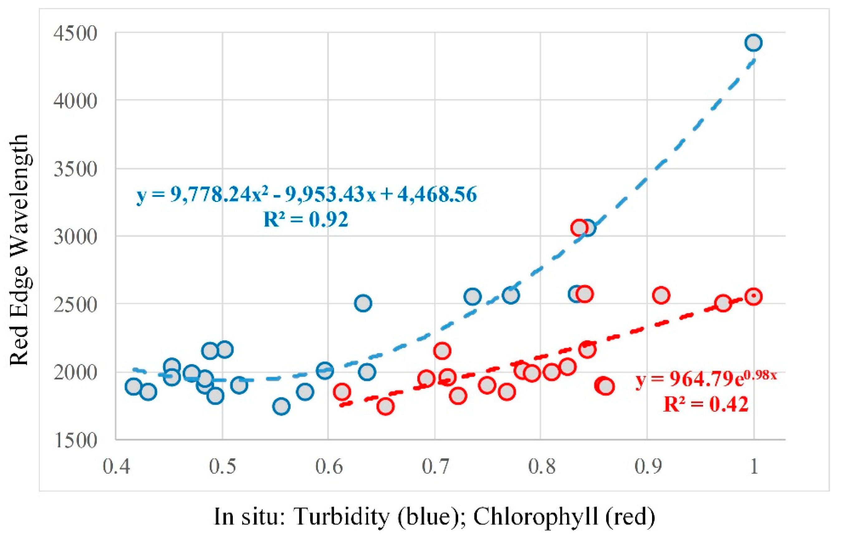
The main results of the study showed a significant relation between RapidEye bands and in situ and laboratory measurements. Similar to different studies, it was concluded that the most useful spectral information, needed to retrieve different water quality parameters are the red and NIR part of the spectrum [38,39]. However, our study also showed that red-edge part of the spectrum is more useful than the NIR for some of the parameters. For example, while EC and TDS showed higher correlation with the NIR band, all of the other parameters showed significant higher correlation with the red-edge band. The 690–730 wavelength range has been widely used in water quality monitoring [31], supporting our findings in Table 5.

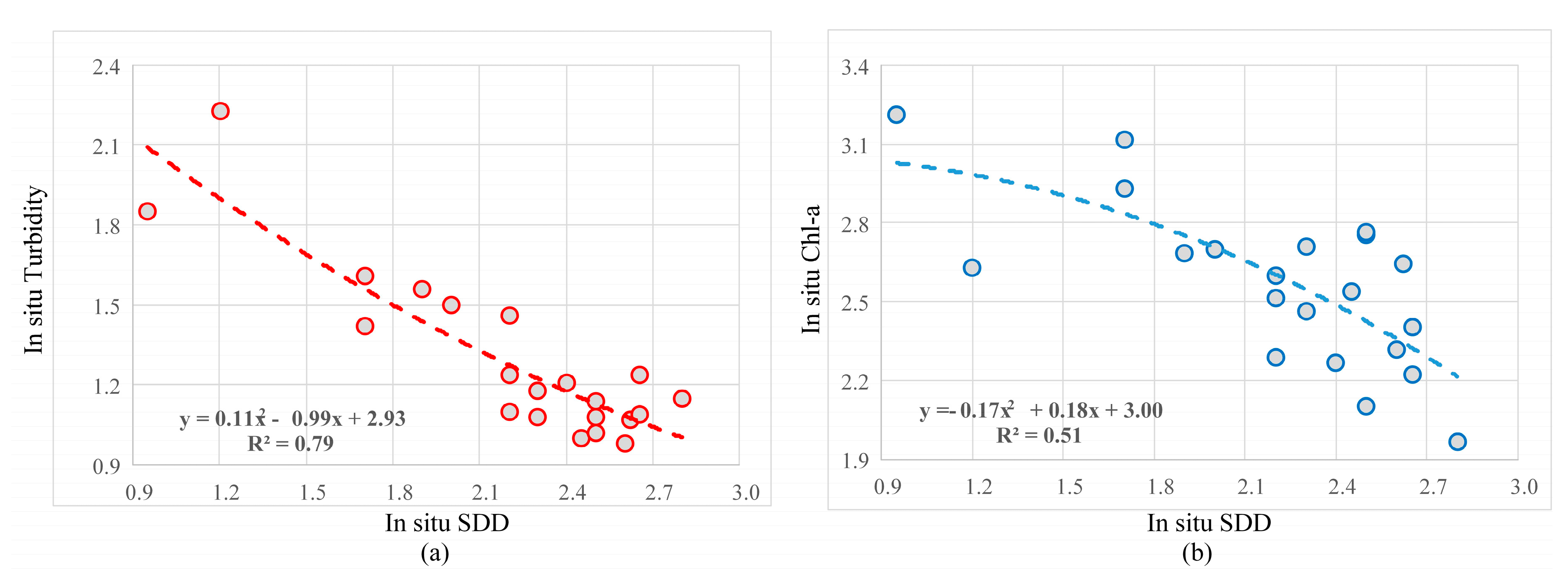
As expected, I1 or NDWI, gave significant results in the water quality parameters. Although it was strongly suggested that it can be used for both water bodies extraction and turbidity monitoring [24], the results in this study indicate that turbidity can be better monitored through a combination of red and green bands. Taking into consideration the higher correlation of red-edge bands with chlorophyll-a rather than NIR, similar to NDCI, I2 was constructed from green and red-edge bands. I5, a green–red ratio, which is also widely used for chlorophyll-a monitoring, gave lower correlation than I2. Also, I2 performed best with a linear correlation of R2 = 0.37. In the literature, I3 (a combination of red and green bands) has been used for both chlorophyll-a and turbidity estimation. The results in this study showed that I3 gave second-best result in the turbidity estimation among all of the investigated indices (R = 0.92), while in the chlorophyll-a estimation was ranked as third (R = 0.54).

The results in this study are slightly better than similar investigations; for example, Masocha et al. [8] found that blue–red ratio provided strong positive relation between measured and retrieved turbidity in two different lakes (R = 0.90; R = 0.80). Different turbidity retrieval approaches showed a good correlation for two different study areas (R = 0.81) [40].

The findings emphasize the use of both high-resolution remote sensing imagery and the red-edge portion of the electromagnetic spectrum for monitoring several water quality parameters in small water areas. Also, this study represents another case study that confirms the use of satellite remote sensing in water quality mapping and monitoring.

5. Conclusions

The presented study assessed the ability of high-resolution satellite sensor to monitor several water quality parameters in small water bodies, such as Borabey Lake in Eskisehir, Turkey. The relation between the in situ measurements, as well as the relation between each RapidEye band, and indices retrieved from RapidEye data were investigated. The main findings of this study proved the ability of RapidEye sensor in water quality estimation with high correlation between the in situ data and the RapidEye reflectance. The results showed a high sensitivity of the water quality parameters in the red, red-edge, and NIR part of the spectrum. The highest correlation has been noticed between in situ turbidity and the red-edge band (r² = 0.92). Also, among the investigated water quality indices, the highest correlation was noticed for turbidity estimation (r² = 0.88).

Investigating different indices, widely used in the literature, it was concluded that some are more successful than others. Thus, although some of the indices were used for both chlorophyll-a and turbidly estimation (I3), the finding of this study showed that chlorophyll-a can be best observed with combination of green and red-edge bands, while good turbidity estimation can be obtained with combination of red and green portions of the spectrum (I3 and I6). As expected, the same combination can be used for estimating water transparency. No significant correlation between red and red-edge bands was observed.

In order to improve the results of this study, a higher number of in situ measurements may be needed. Also, different water quality parameters with high-resolution satellite imagery should be observed. As the algorithms used in this study are easy to implement, we recommend further analyses in different study areas at different seasons of the year in order to get a wider range of values of water quality. Similar studies should be conducted in both turbid and clear water in order to support the results and encourage remote sensing data in water quality monitoring.

References

1. Su, Z.; Yacob, A.; Wen, J.; Roerink, G.; He, Y.; Gao, B.; Voogaard, H.; van Diepen, C. Assessing relative soil moisture with remote sensing data: Theory, experimental validation, and application to drought monitoring over the North China Plain. Phys. Chem. Earth Parts A/B/C 2003, 28, 89–101. [Google Scholar] [CrossRef]
2. Crétaux, J.F.; Jelinski, W.; Calmant, S.; Kouraev, A.; Vuglinski, V.; Bergé-Nguyen, M.; Gennero, M.-C.; Nino, F.; Del Rio Abarca, R.; Cazenave, A.; et al. SOLS: A lake database to monitor in the Near Real Time water level and storage variations from remote sensing data. Adv. Space Res. 2011, 47, 1497–1507. [Google Scholar] [CrossRef]
3. Ines, A.V.; Honda, K.; Gupta, A.D.; Droogers, P.; Clemente, R.S. Combining remote sensing-simulation modeling and genetic algorithm optimization to explore water management options in irrigated agriculture. Agric. Water Manag. 2006, 83, 221–232. [Google Scholar] [CrossRef]
4. Feng, Q.; Liu, J.; Gong, J. Urban flood mapping based on unmanned aerial vehicle remote sensing and random forest classifier—A case of Yuyao, China. Water 2015, 7, 1437–1455. [Google Scholar] [CrossRef]
5. Andres, L.; Boateng, K.; Borja-Vega, C.; Thomas, E. A review of in situ and remote sensing technologies to monitor water and sanitation interventions. Water 2018, 10, 756. [Google Scholar] [CrossRef]
6. Amitrano, D.; Martino, G.; Iodice, A.; Mitidieri, F.; Papa, M.; Riccio, D.; Ruello, G. Sentinel-1 for monitoring reservoirs: A performance analysis. Remote Sens. 2014, 6, 10676–10693. [Google Scholar] [CrossRef]
7. Kaplan, G.; Avdan, U. Water extraction technique in mountainous areas from satellite images. J. Appl. Remote Sens. 2017, 11, 046002. [Google Scholar] [CrossRef]
8. Masocha, M.; Dube, T.; Nhiwatiwa, T.; Choruma, D. Testing utility of Landsat 8 for remote assessment of water quality in two subtropical African reservoirs with contrasting trophic states. Geocarto Int. 2018, 33, 667–680. [Google Scholar] [CrossRef]
9. Kaplan, G.; Avdan, U. Object-based water body extraction model using Sentinel-2 satellite imagery. Eur. J. Remote Sens. 2017, 50, 137–143. [Google Scholar] [CrossRef]
10. Ogashawara, I.; Moreno-Madriñán, M. Improving inland water quality monitoring through remote sensing techniques. ISPRS Int. J. Geo-Inf. 2014, 3, 1234–1255. [Google Scholar] [CrossRef]
11. Ha NT, T.; Thao NT, P.; Koike, K.; Nhuan, M.T. Selecting the Best Band Ratio to Estimate Chlorophyll-a Concentration in a Tropical Freshwater Lake Using Sentinel 2A Images from a Case Study of Lake Ba Be (Northern Vietnam). ISPRS Int. J. Geo-Inf. 2017, 6, 290. [Google Scholar]
12. Fischer, A.; Pang, D.; Kidd, I.; Moreno-Madriñán, M. Spatio-temporal variability in a turbid and dynamic tidal estuarine environment (Tasmania, Australia): An assessment of MODIS band 1 reflectance. ISPRS Int. J. Geo-Inf. 2017, 6, 320. [Google Scholar] [CrossRef]
13. Politi, E.; Prairie, Y.T. The potential of Earth Observation in modelling nutrient loading and water quality in lakes of southern Québec, Canada. Aquat. Sci. 2018, 80, 8. [Google Scholar] [CrossRef]
14. Koparan, C.; Koc, A.; Privette, C.; Sawyer, C. In situ water quality measurements using an unmanned aerial vehicle (UAV) system. Water 2018, 10, 264. [Google Scholar] [CrossRef]
15. Dogan, H.M.; Polat, F.; Buhan, E.; Kiliç, O.M.; Yilmaz, D.; Buhan, S.D. Modeling and Mapping Temperature, Secchi Depth, and Chlorophyll-a Distributions of Zinav Lake by Using GIS and Landsat-7 ETM+ Imagery. J. Agric. Fac. Gaziosmanpasa Univ. 2016, 33, 55–60. [Google Scholar]
16. Kabbara, N.; Benkhelil, J.; Awad, M.; Barale, V. Monitoring water quality in the coastal area of Tripoli (Lebanon) using high-resolution satellite data. ISPRS J. Photogramm. Remote Sens. 2008, 63, 488–495. [Google Scholar] [CrossRef]
17. Dogliotti, A.I.; Ruddick, K.G.; Nechad, B.; Doxaran, D.; Knaeps, E. A single algorithm to retrieve turbidity from remotely-sensed data in all coastal and estuarine waters. Remote Sens. Environ. 2015, 156, 157–168. [Google Scholar] [CrossRef]
18. Ehmann, K.; Kelleher, C.; Condon, L.E. Monitoring turbidity from above: Deploying small unoccupied aerial vehicles to image in-stream turbidity. Hydrol. Process. 2019, 33, 1013–1021. [Google Scholar] [CrossRef]
19. Brezonik, P.; Menken, K.D.; Bauer, M. Landsat-based remote sensing of lake water quality characteristics, including chlorophyll and colored dissolved organic matter (CDOM). Lake Reserv. Manag. 2005, 21, 373–382. [Google Scholar] [CrossRef]
20. Robert, E.; Kergoat, L.; Soumaguel, N.; Merlet, S.; Martinez, J.M.; Diawara, M.; Grippa, M. Analysis of suspended particulate matter and its drivers in Sahelian ponds and lakes by remote sensing (Landsat and MODIS): Gourma region, Mali. Remote Sens. 2017, 9, 1272. [Google Scholar] [CrossRef]
21. He, X.; Pan, D.; Bai, Y.; Wang, T.; Chen, C.-T.A.; Zhu, Q.; Hao, Z.; Gong, F. Recent changes of global ocean transparency observed by SeaWiFS. Cont. Shelf Res. 2017, 143, 159–166. [Google Scholar] [CrossRef]
22. Kaya, M. Interaction of Water Quality with Basin Components in Small Water Bodies. Master’s Thesis, Anadolu University, Eskisehir, Turkey, 2012. [Google Scholar]
23. Planet Application Program Interface: In Space for Life on Earth; Team Planet: San Francisco, CA, USA, 2017; Volume 2017, p. 40.
24. McFeeters, S.K. The use of the Normalized Difference Water Index (NDWI) in the delineation of open water features. Int. J. Remote Sens. 1996, 17, 1425–1432. [Google Scholar] [CrossRef]
25. Watanabe, F.; Alcantara, E.; Rodrigues, T.; Rotta, L.; Bernardo, N.; Imai, N. Remote sensing of the chlorophyll-a based on OLI/Landsat-8 and MSI/Sentinel-2A (Barra Bonita reservoir, Brazil). An. Acad. Bras. Ciências 2018, 90, 1987–2000. [Google Scholar] [CrossRef] [PubMed]
26. Elhag, M.; Gitas, I.; Othman, A.; Bahrawi, J.; Gikas, P. Assessment of Water Quality Parameters Using Temporal Remote Sensing Spectral Reflectance in Arid Environments, Saudi Arabia. Water 2019, 11, 556. [Google Scholar] [CrossRef]
27. Lacaux, J.P.; Tourre, Y.M.; Vignolles, C.; Ndione, J.A.; Lafaye, M. Classification of ponds from high-spatial resolution remote sensing: Application to Rift Valley Fever epidemics in Senegal. Remote Sens. Environ. 2007, 106, 66–74. [Google Scholar] [CrossRef]
28. Mishra, S.; Mishra, D.R. Normalized difference chlorophyll index: A novel model for remote estimation of chlorophyll-a concentration in turbid productive waters. Remote Sens. Environ. 2012, 117, 394–406. [Google Scholar] [CrossRef]
29. Mishra, D.R.; Schaeffer, B.A.; Keith, D. Performance evaluation of normalized difference chlorophyll index in northern Gulf of Mexico estuaries using the Hyperspectral Imager for the Coastal Ocean. GISci. Remote Sens. 2014, 51, 175–198. [Google Scholar] [CrossRef]
30. Kallio, K.; Attila, J.; Härmä, P.; Koponen, S.; Pulliainen, J.; Hyytiäinen, U.M.; Pyhälahti, T. Landsat ETM+ images in the estimation of seasonal lake water quality in boreal river basins. Environ. Manag. 2008, 42, 511–522. [Google Scholar] [CrossRef]
31. Toming, K.; Kutser, T.; Uiboupin, R.; Arikas, A.; Vahter, K.; Paavel, B. Mapping water quality parameters with sentinel-3 ocean and land colour instrument imagery in the Baltic Sea. Remote Sens. 2017, 9, 1070. [Google Scholar] [CrossRef]
32. Abdelmalik, K. Role of statistical remote sensing for Inland water quality parameters prediction. Egypt. J. Remote Sens. Space Sci. 2018, 21, 193–200. [Google Scholar] [CrossRef]
33. Koponen, S.; Attila, J.; Pulliainen, J.; Kallio, K.; Pyhälahti, T.; Lindfors, A.; Rasmus, K.; Hallikainen, M. A case study of airborne and satellite remote sensing of a spring bloom event in the Gulf of Finland. Cont. Shelf Res. 2007, 27, 228–244. [Google Scholar] [CrossRef]
34. Yadav, S.; Yamashiki, Y.; Susaki, J.; Yamashita, Y.; Ishikawa, K. Chlorophyll Estimation of Lake Water and Coastal Water Using LANDSAT-8 and SENTINEL-2A Satellite. Int. Arch. Photogramm. Remote Sens. Spat. Inf. Sci. 2019, 42. [Google Scholar] [CrossRef]
35. Bonansea, M.; Ledesma, M.; Rodriguez, C.; Pinotti, L. Using new remote sensing satellites for assessing water quality in a reservoir. Hydrol. Sci. J. 2019, 64, 34–44. [Google Scholar] [CrossRef]
36. Gürsoy, Ö.; Atun, R. Investigating Surface Water Pollution by Integrated Remotely Sensed and Field Spectral Measurement Data: A Case Study. Pol. J. Environ. Stud. 2019, 28, 2139–2144. [Google Scholar] [CrossRef]
37. Vanhellemont, Q. Daily metre-scale mapping of water turbidity using CubeSat imagery. Opt. Express 2019, 27, A1372–A1399. [Google Scholar] [CrossRef]
38. Alikas, K.; Kratzer, S.; Reinart, A.; Kauer, T.; Paavel, B. Robust remote sensing algorithms to derive the diffuse attenuation coefficient for lakes and coastal waters. Limnol. Oceanogr. Methods 2015, 13, 402–415. [Google Scholar] [CrossRef]
39. Paavel, B.; Arst, H.; Metsamaa, L.; Toming, K.; Reinart, A. Optical investigations of CDOM-rich coastal waters in Pärnu Bay. Est. J. Earth Sci. 2011, 60, 102. [Google Scholar] [CrossRef]
40. Güttler, F.N.; Niculescu, S.; Gohin, F. Turbidity retrieval and monitoring of Danube Delta waters using multi-sensor optical remote sensing data: An integrated view from the delta plain lakes to the western–northwestern Black Sea coastal zone. Remote Sens. Environ. 2013, 132, 86–101. [Google Scholar] [CrossRef] [Green Version]
Figure 1. Study Area, Borabey Lake (left; RapidEye image, RGB - 3,5,1), Eskisehir, Turkey.
Ijgi 08 00553 g001
Figure 2. RapidEye-3 image of Borabey Lake, and locations of in situ measurements.
Ijgi 08 00553 g002
Figure 3. Relationship between: (a) SDD and turbidity; (b) SDD and chlorophyll-a.
Ijgi 08 00553 g003
Figure 4. Relationship between red edge wavelength and in situ turbidity (blue); and chlorophyll-a (red).
Ijgi 08 00553 g004
Figure 5. Correlation between estimated and actual water quality parameters (I1-I8 are shown in Table 3).
Ijgi 08 00553 g005