Clustering Complex Trajectories Based on Topologic Similarity and Spatial Proximity: A Case Study of the Mesoscale Ocean Eddies in the South China Sea

Abstract

Many real-world dynamic features such as ocean eddies, rain clouds, and air masses may split or merge while they are migrating within a space. Topologically, the migration trajectories of such features are structurally more complex as they may have multiple branches due to the splitting and merging processes. Identifying the spatial aggregation patterns of the trajectories could help us better understand how such features evolve. We propose a method, a Global Similarity Measuring Algorithm for the Complex Trajectories (GSMCT), to examine the spatial proximity and topologic similarity among complex trajectories. The method first transforms the complex trajectories into graph structures with nodes and edges. The global similarity between two graph structures (i.e., two complex trajectories) is calculated by averaging their topologic similarity and the spatial proximity, which are calculated using the Comprehensive Structure Matching (CSM) and the Hausdorff distance (HD) methods, respectively. We applied the GSMCT, the HD, and the Dynamic Time Warping (DTW) methods to examine the complex trajectories of the 1993–2016 mesoscale eddies in the South China Sea (SCS). Based on the similarity evaluation results, we categorized the complex trajectories across the SCS into four groups, which are similar to the zoning results reported in previous studies, though difference exists. Moreover, the yearly numbers of complex trajectories in the clusters in the northernmost (Cluster 1) and the southernmost SCS (Cluster 4) are almost the same. However, their seasonal variation and migration characteristics are totally opposite. Such new knowledge is very useful for oceanographers of interest to study and numerically simulate the mesoscale ocean eddies in the SCS.

1. Introduction

Analysis of trajectories and their patterns has drawn much attention from data scientists [1,2]. It has been widely seen in behavioral science, transportation engineering, biology, meteorology, oceanography, and many other disciplines [3,4,5]. As one of the most widely used methods to unravel trajectory patterns, trajectory clustering seeks to minimize the difference among trajectories within a cluster, while maximizing the difference between clusters [6,7,8,9]. Trajectory clustering has been used to explore population migration patterns [6,7,8], human activities and behavior abnormalities, urban vehicle movement characteristics, cell development processes, and atmospheric evolution processes [5,6,7,8,9,10,11]. There is a need for a feasible definition of trajectory similarity measure for successful trajectory clustering, trajectory classification, pattern analysis, and movement anomaly detection [3,8,9].

Migration of real-world entities has been widely traced and a huge amount of trajectory data have been produced [12]. A trajectory could be either simple or complex, depending upon whether it has branches or not [5,11]. The branches are produced when the entities split and/or merge. A simple trajectory (Figure 1a) is usually generated by an object that moves as a whole, such as a person, a vehicle, or an animal. A simple trajectory thus has a linear structure without any branches [3,6,7,9,10]. By contrast, a complex trajectory (Figure 1b) is structurally different from a simple trajectory in that it has nonlinear structure with at least one branch. A complex trajectory is usually generated by the phenomena that could split or merge, such as large-scale ocean eddies, rain clouds, and air masses [13,14,15], and even the micro-scale cells [11]. More studies have been done on the simple rather than the complex trajectories. When studying complex trajectories, scientists usually break a complex trajectory into multiple simple trajectories and then examine the simple trajectories separately [14]. There has been a lack of methods that could be used to examine the similarity between complex trajectories as a whole.

Simple trajectories are usually clustered based on their spatial proximity. By contrast, complex trajectories share both spatial and topologic similarity. A variety of methods have been developed and used to evaluate the spatial similarity between trajectories. The equal-length ordered comparison methods [16,17] are usually utilized to measure the similarity between trajectories with the same number of points. The smaller the sum or the average of the Euclidean distances between the corresponding time series points along the trajectories, the more similar the trajectories are [16,17]. However, these methods cannot be used to measure the similarity between most complex trajectories in that the numbers of the points along two complex trajectories are seldom to be exactly the same.

Methods have also been developed to evaluate trajectory similarity by optimally matching the points along the trajectories based on their locations in the time series. Such methods are also known as the unequal length ordered comparison methods, such as the Fréchet Distance, the Dynamic Time Warping (DTW), and the Longest Common Sub-Sequence (LCSS) distance [8,9,18,19,20] methods, which iteratively seek to optimally match the trajectory points which are arranged chronologically. This group of methods usually requires a premise that the moves of an object must exactly match the points that the moves generate along the trajectory at a specific time. Unfortunately, such a premise may not always be true for complex trajectories.

The third group of methods evaluates trajectory similarity by matching the points along trajectories without considering their chronological order [9]. One of the widely used methods is Hausdorff Distance (HD) [6,16], which uses the bidirectional Hausdorff distance H(A, B), i.e., the larger value of the one-way distance h(A, B) and h(B, A), to measure the maximum mismatch between two point sets A and B along trajectories. This group of methods could be directly applied to measure the spatial similarity among complex trajectories.

In addition to the spatial similarity, complex trajectories also share topologic similarity, which measures structurally how similar two trajectories could be. The trajectories are first translated to graphs. The topologic similarity of the trajectories is then evaluated by matching the common structures and the corresponding attributes of the graphs [21]. The graph isomorphism algorithm VF2 [22] has been widely used to match the common structures on the basis of graph isomorphism (two graphs share the exactly same structure) and subgraph isomorphism (one graph is a subgraph of another). However, graphs may also show partial isomorphism (two graphs are partially the same regarding their structures), which is not considered by the VF2 method. Inspired by the VF2 method, our research group has proposed a new method, Comprehensive Structure Matching (CSM), for measuring the topologic similarity between two complex trajectories [5]. CSM takes into account all of the three aforementioned graph, subgraph, and partial isomorphism.

It is worthy to note that the CMS method does not consider the spatial proximity. In this paper, we propose a new method, Global Similarity Measuring Algorithms for Complex Trajectories (GSMCT), to measure both the spatial proximity and topological similarity of complex trajectories. The method was applied to examine the complex trajectories of the 1993–2016 mesoscale ocean eddies in the South China Sea (SCS). It has been well documented that ocean eddies in the SCS split and merge frequently [13,23,24], producing many complex trajectories that are perfect for evaluation of our new method. Eddy splitting events usually lead to current deformation, material dispersion, and subsequent energy decay, which all affect water temperature and salinity, and, consequently, the marine ecosystems [23]. By contrast, eddy merging events enhance seawater interaction in different regions and thus affect the trans-scale transmission of energy and entropy in turbulence [24]. In a broader context, the splitting and merging activities of mesoscale ocean eddies could significantly affect transmission and exchange of energy and matter in the oceans, and thus play an important role in marine ecosystems, atmospheric environment, and surface ocean circulation [25]. Many other complex dynamic phenomena, such as storms, clouds, and air masses, may also split and merge frequently [13,14,15] and generate complex trajectories that are very similar to those of the mesoscale eddies. We believe it is perfect to use the mesoscale eddies’ complex trajectories to test the GSMCT algorithm, which then could be used to study complex trajectories of other dynamic phenomena.

Many studies have been conducted to explore the static and dynamic characteristics of the mesoscale ocean eddies in the SCS using different datasets and methods [24,26,27,28]. On the one hand, some studies focus on the formation mechanism, spatial distribution, seawater interaction, and physical properties of a single eddy or a specific type of eddy in the SCS [13,29,30]. On the other hand, some studies perform spatiotemporal statistical and clustering analysis on all eddies [26,28,31]. To a certain extent, the previous studies have revealed the spatiotemporal characteristics and patterns, overall migration trend and channels of the SCS ocean eddies. However, very few, if any, previous studies ever tried to study complex ocean eddy trajectories generated by eddy splitting and merging activities in the SCS separately, though it has been well documented that splitting and merging are very important in studying ocean water interaction, material and energy transfer [23,24]. In this study, we applied our new proposed method to examine the complex eddy trajectories in the SCS with an aim to better reveal how the simple and complex eddy trajectories are different in the SCS.

The remainder of this paper is organized as follows: Section 2 defines the complex trajectories and presents the methodology. Section 3 presents a real-world application and the new knowledge produced in this study. Section 4 mainly discusses the advantages and disadvantages of the GSMCT method. Section 5 presents the major conclusions of this study and also briefly outlines our future research thoughts.

2. Definitions and Methodology

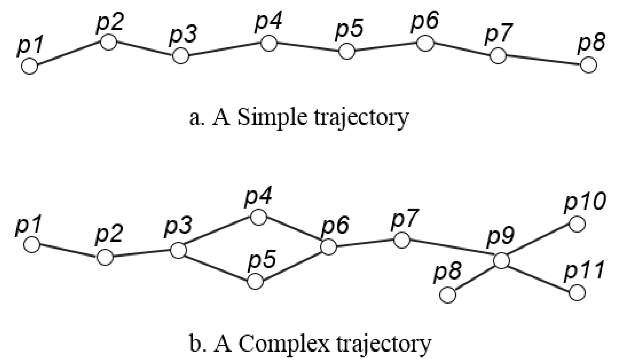
2.1. Definitions of Simple and Complex Trajectories

The definitions of simple and complex trajectories in [5] were refined as follows for the purpose of more accurately presenting their difference in terms of their topologic structures.

Definition 1.

A simple trajectory consists of a series of points in a chronological order and shows a linear structure (Figure 1a). Every move of an object at a specific time generates one point along the trajectory, as shown below:

$$ST{r}_i=\left\{\right(P_1,x_1,y_1,t_1);(P_2,x_2,y_2,t_2);\cdots (P_i,y_i{t}_i\left)\right\}$$

where i is the number of the points along a simple trajectory, P_i is the ID of the ith trajectory point, x_i, and y_i represent the spatial location (the coordinates) of the trajectory point i, and t_i represents the specific timestamp of the trajectory point i.

Definition 2.

In this study, the complex trajectories are defined as those with branches, which are generated when an object splits into more than one individual or multiple objects merge into one individual at a specific timestamp (Figure 1b). Unlike a simple trajectory, a complex trajectory has a nonlinear structure and can be defined as follows:

$$CT{r}_j=\left\{\right(P_1,x_1,y_1,t_1,P_{\mathit{type}},P_{\mathit{next}});(P_2,x_2,y_2,t_2,P_{\mathit{type}},P_{\mathit{next}});\cdots P_j,y_j,P_{\mathit{type}},P_{\mathit{next}})\}$$

where j is the number of the points along a complex trajectory; P_j, x_j, y_j, and t_j represent the same as those in a simple trajectory, respectively; P_next represents the ID of the successor point; and P_type represents the type of a point along a complex trajectory. A point along a complex trajectory could be a(an) starting, ending, splitting, merging, merge–split point, or common point. Any non-starting, ending, splitting, merging, split–merge points are defined as common points in this study. In Figure 1b, p1 and p8 are starting points. Points p10 and p11 are ending points. Points p2 and p7 are common points. Points p3, p6, and p9 are splitting, merging, and merge–split points, respectively. Obviously, there are only starting, ending, and common points along a simple trajectory.

In addition to the types the points could be, a complex trajectory is also different from a simple trajectory in terms of the relationship between the moves of an object and the points the moves generated along the trajectory. Along a simple trajectory, every move of an object at a specific time generates one point along the trajectory. By contrast, one move of the object could generate multiple points along a complex trajectory.

A simple trajectory can also be distinguished from a complex trajectory in terms of its complexity. In this study, the complexity of a trajectory (η, 0 < η ≤ 1) is defined as the ratio between the number of the points along the branches and the total number of the points along the major trajectory and all connected branches. A simple trajectory has a complexity of 0. The complexity of a complex trajectory ranges between 0 and 1, depending on how complicated its structure is. The trajectory illustrated in Figure 1b has 11 points in total along the whole trajectory and 9 out of them are on the branches. Its trajectory complexity η is therefore 0.818.

2.2. Methodology

The essential idea of our method is to cluster complex trajectories based on their topologic similarity and spatial proximity. The topologic similarity is the maximum similarity of the trajectory topologic structures and is calculated using the CSM algorithm proposed in one of our previous studies [5]. The spatial proximity is calculated using the HD method [6,16]. We then hierarchically grouped the complex trajectories based on the similarity results. In the end, we evaluated the clustering results using the Calinski–Harabasz method [32].

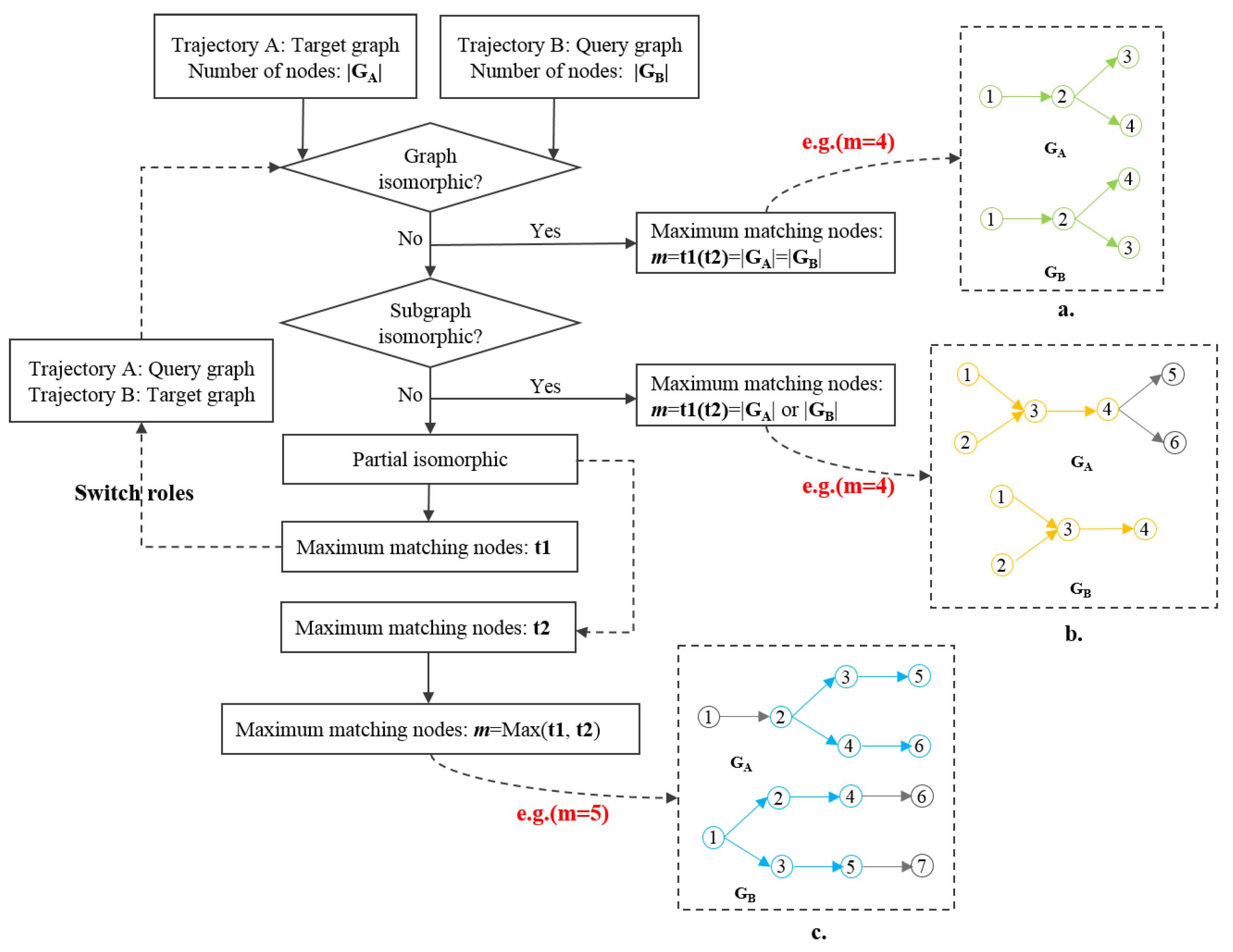
2.2.1. Topologic Similarity

Topologically, a complex trajectory could be translated to a directional acyclic graph (DAG) with a variety of nodes and edges. In this study, the structure of a DAG is defined as follows.

Definition 3.

The DAG of a complex trajectory is a 2-tuple G = (N, E).

where N is a set of finite nodes, E ⊆ N × N is the set of edges, and |G| is the number of the nodes in the graph.

We first used our CSM algorithm [5] to identify all common structures in the complex trajectories of interest. Essentially, the CSM algorithm measures the similarity between trajectories by comparing their DAGs in terms of the graph isomorphism (Figure 2a), subgraph isomorphism (Figure 2b), and partial isomorphism (Figure 2c), as shown in Figure 2.

Given two complex trajectories, A and B, their DAGs could be defined as G_A = (N_A, E_A) and G_B = (N_B, E_B), respectively. The node numbers of G_A and G_B are |G_A| and |G_B|, respectively. We first defined G_A and G_B as the target and query graphs, respectively. The CSM compares the two graphs and identifies whether they are graph isomorphic, subgraph isomorphic, or partial isomorphic. It then calculates the maximum number of the nodes (t₁) in the matching common structure between the target graph A and the query graph B. We then swapped the roles of G_A and G_B, repeated the aforementioned procedure, and calculated the maximum number of the nodes (t₂) in the matching common structure between the target graph B and the query graph A.

If G_A and G_B are graph isomorphic, the numbers of the nodes in G_A and G_B would be the same (i.e., |G_A| = |G_B|) and the maximum number of matching nodes m would be the number of the nodes in graph A or B (i.e., m = t₁ = t₂). If G_A and G_B are subgraph isomorphic, the query graph would be a part of the structure of the target graph, and m would be the number of the nodes in the query graph. If G_A and G_B are partially graph isomorphic, m would be the larger values of t₁ and t₂.

The Jaccard similarity coefficient [5] is then used to calculate the topologic similarity between the complex trajectories A and B, as shown below.

$$Si{m}_{TOP}\left(\mathrm{A},\mathrm{B}\right)= m/\left(\left|{\mathrm{G}}_{\mathrm{A}}\right|+\left|{\mathrm{G}}_{\mathrm{B}}\right|-m\right)$$

(1)

$$\left(0\le Si{m}_{TOP}\left(\mathrm{A},\mathrm{B}\right)\le 1\right)$$

where G_A and G_B are the graphs representing the complex trajectories A and B, respectively. |G_A| and |G_B| are the total numbers of the nodes in G_A and G_B, respectively. G_A ∩ G_B is the size of the intersection between G_A and G_B, i.e., the maximum number (m) of the matched nodes between the two complex trajectories. The similarity (G_A, G_B) would be 1 if G_A and G_B are graph isomorphic. If G_A is a subgraph of G_B, the similarity (G_A, G_B) would be G_A/G_B.

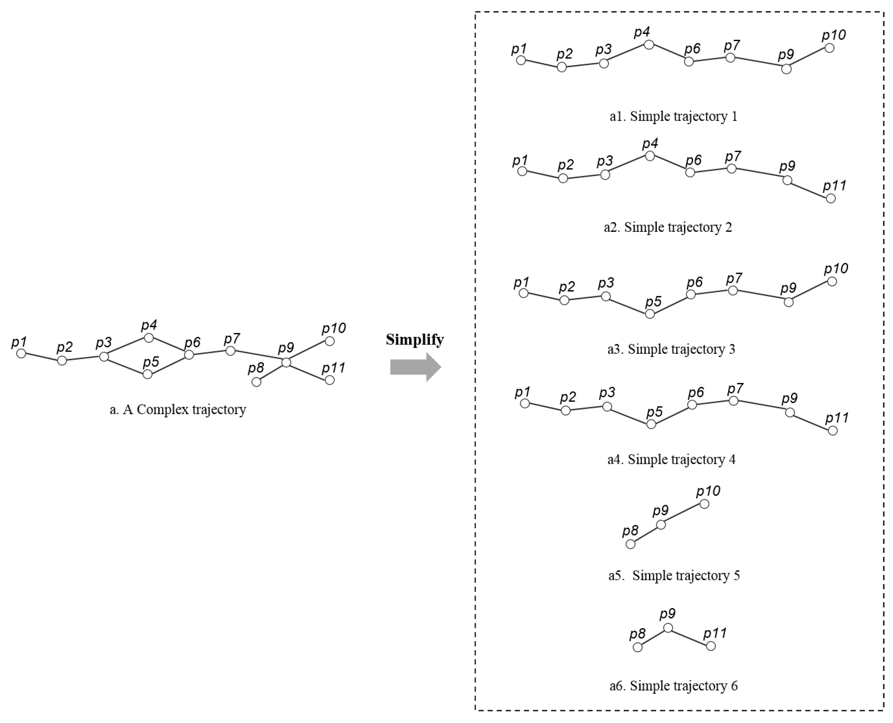
2.2.2. Distance Measurement Between Complex Trajectories

In addition to the topologic similarity, the two complex trajectories could also be similar in terms of their spatial proximity, which was measured using the HD distance [6,9,16] in this study. The HD measures the similarity between trajectories based on their overall geometric characteristics. The one-way HD h(A, B) from complex trajectories A to B is the maximum of the shortest distances from the points along trajectory A to those along trajectory B. The one-way HD h(B, A) from complex trajectories B to A is the maximum of the shortest distances from the points along trajectory B to those along trajectory A. The two-sided HD H(A, B) is the larger value of the one-way distance h(A, B) and h(B, A), and measures the maximum mismatch between the points along two complex trajectories, as shown below:

$$\mathrm{H}(\mathrm{A},\mathrm{B})=\max \left(h\left(\mathrm{A},\mathrm{B}\right),h\left(\mathrm{B},\mathrm{A}\right)\right)$$

(2)

We then used the min–max normalization method (Equation (3)) to linearly transform H(A, B) to unified $\mathrm{H}{\left(\mathrm{A},\mathrm{B}\right)}^{*}$, which ranges between 0 and 1.

$$\mathrm{H}{\left(\mathrm{A},\mathrm{B}\right)}^{*}=\frac{\mathrm{H}\left(\mathrm{A},\mathrm{B}\right)-\min \left(\mathrm{H}\right)}{\max \left(\mathrm{H}\right)-\min \left(\mathrm{H}\right)}$$

(3)

where $\min \left(\mathrm{H}\right)$ and $\max \left(\mathrm{H}\right)$ represent the minimum and maximum values of the HD between two complex trajectories, respectively. The unified $\mathrm{H}{\left(\mathrm{A},\mathrm{B}\right)}^{*}$ still measures the maximum mismatch between two complex trajectories, and the spatial proximity could then be defined as below [33,34]:

$$Si{m}_{DIS}\mathrm{H}{\left(\mathrm{A},\mathrm{B}\right)}^{*}=1-\mathrm{H}{\left(\mathrm{A},\mathrm{B}\right)}^{*}$$

(4)

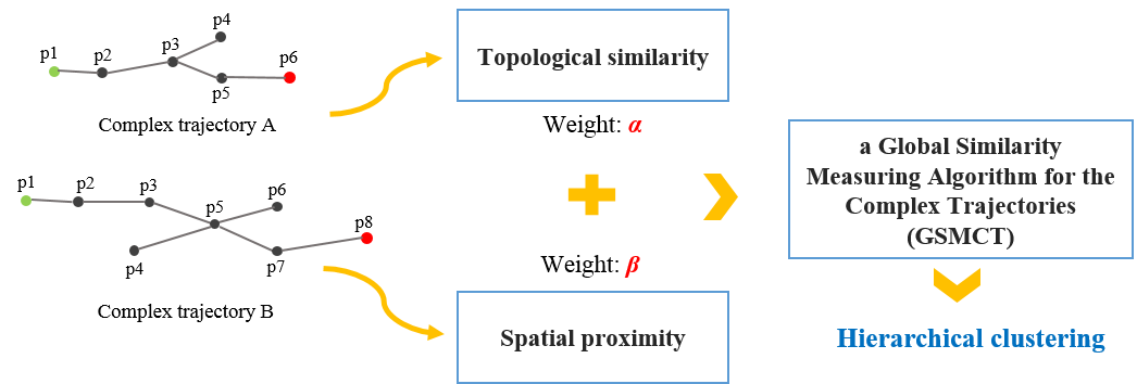
2.2.3. Global Similarity Between Complex Trajectories

The global similarity between two complex trajectories, A and B, was measured by considering both their topologic similarity and spatial proximity, as shown in Equation (5).

$$\mathrm{GSMCT}\left(\mathrm{A},\mathrm{B}\right)=\alpha \left(Si{m}_{TOP}\left(\mathrm{A},\mathrm{B}\right)\right)+\beta \left(Si{m}_{DIS}\mathrm{H}{\left(\mathrm{A},\mathrm{B}\right)}^{*}\right)$$

(5)

$$\left(0\le \mathrm{GSMCT}\left(\mathrm{A},\mathrm{B}\right)\le 1\right)$$

where GSMCT(A,B), $Si{m}_{TOP}\left(\mathrm{A},\mathrm{B}\right)$, and $Si{m}_{DIS}\mathrm{H}{\left(\mathrm{A},\mathrm{B}\right)}^{*}$ are the global similarity, the topological similarity, and the spatial proximity between two complex trajectories, A and B, respectively. The importance of the topologic similarity and the spatial proximity could be adjusted by changing weights α and β, where α + β = 1, by default, α = β = 0.5.

2.2.4. Hierarchical Clustering Based on the Global Similarity

We then clustered the complex trajectories based on their global similarity values. Each complex trajectory is initially treated as a separate cluster. A global dissimilarity (i.e., 1-GSMCT(A,B)) matrix is constructed to show the dissimilarity between any pair of complex trajectories. The average-linkage agglomerative hierarchical clustering method [35] was then used to merge the clusters from bottom to top by first calculating the average of the dissimilarity between trajectories within two clusters and then iterating the process until only one cluster is left. Finally, the Calinski–Harabasz Index [32] was used to determine the optimal number of clusters and evaluate the clustering results. The Calinski–Harabasz Index is calculated as follows:

$$\mathrm{CHk}=\frac{S{S}_B}{S{S}_w}\times \frac{N-k}{k-1}$$

(6)

where $S{S}_B$ and $S{S}_w$ are the overall variance between clusters and within a specific cluster. k and N are the numbers of the clusters and the total number of complex trajectories participating the cluster analysis, respectively. A larger $\mathrm{CHk}$ would indicate a smaller covariance within a cluster and a greater covariance between the clusters, and thus a better clustering result. A series of $\mathrm{CHk}$ values could be calculated assuming the complex trajectories were grouped into different clusters. The optimal cluster number would be the number of clusters (k) when a maximum $\mathrm{CHk}$ value was found.

In fact, other indexes such as the Davies–Bouldin Index and silhouette coefficient [36] could also be used to determine the optimal number of clusters. However, the Calinski–Harabasz Index better fits our dataset, because its computing speed is hundreds of times faster than the Davies–Bouldin Index and silhouette coefficient [36]. Furthermore, the Davies–Bouldin Index and silhouette coefficient evaluate the clustering results by calculating the Euclidean distance based on the geometry structure of the dataset. The Euclidean distance was taken into account when we calculated the spatial proximity between complex trajectories, and should not be used again in determining the optimal clustering number. As a result, we used the Calinski–Harabaz Index in this study to determine the optimal clustering number.

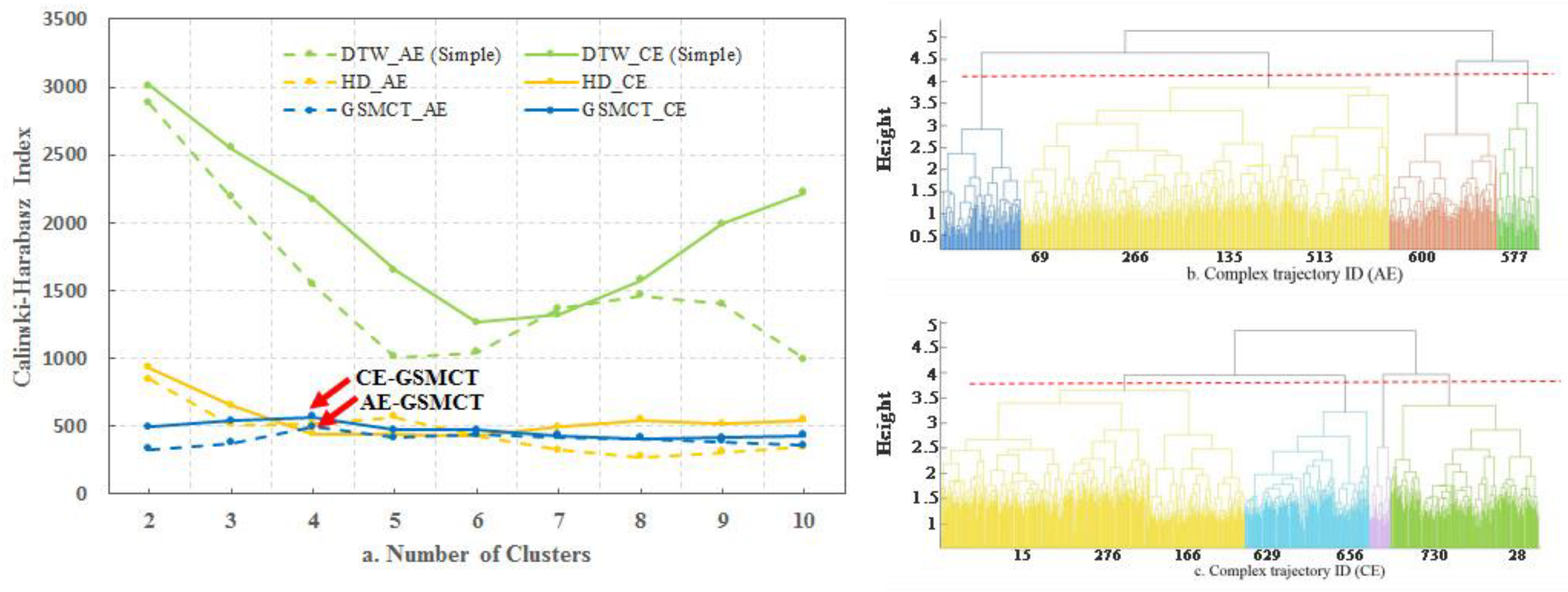
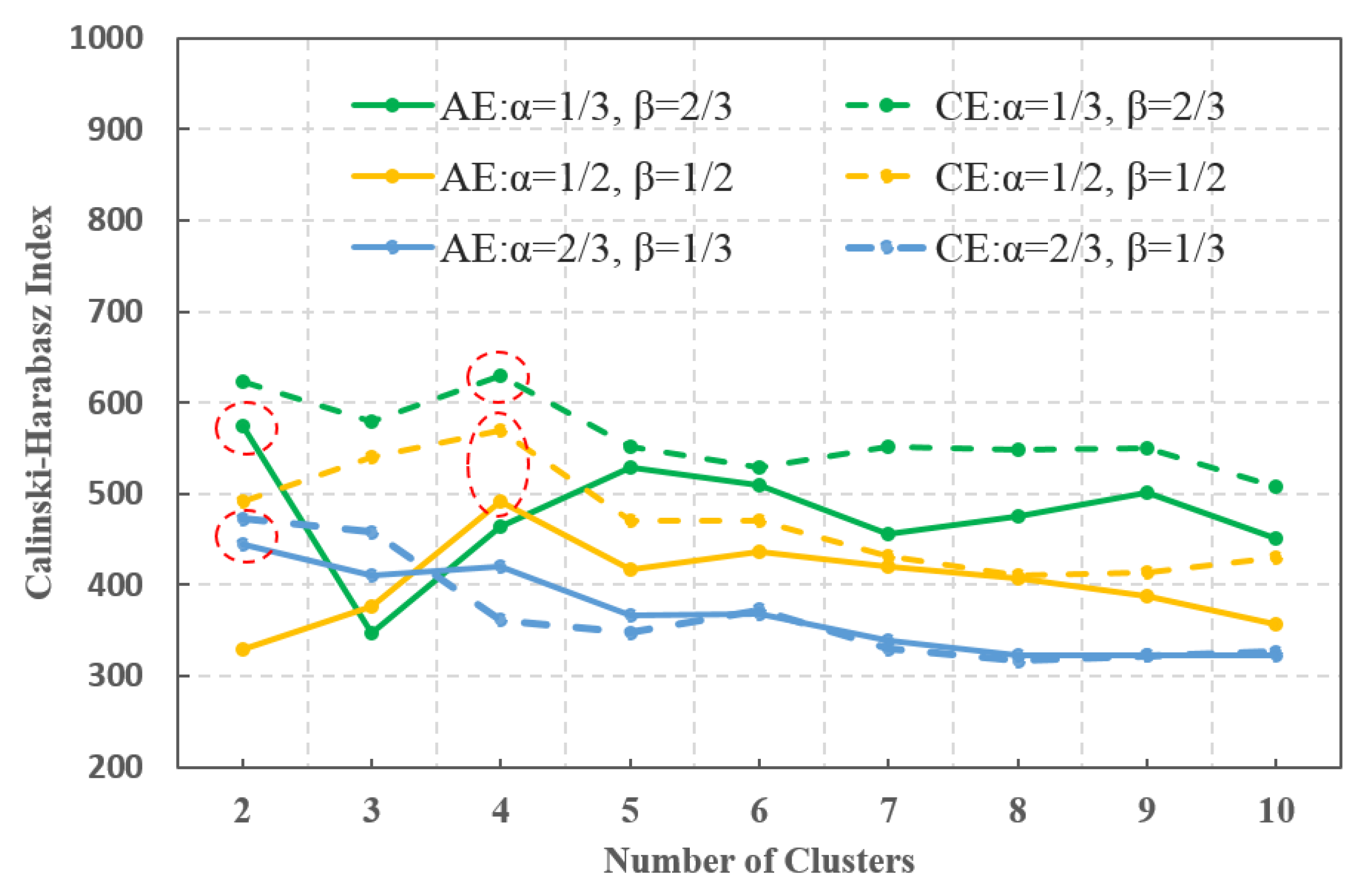
2.2.5. Method Comparison and Evaluation of Results

We compared the performance of our GSMCT method in evaluating similarity of complex trajectories against the HD and the DTW methods [7,20]. We described the HD method in Section 2.2.2. The DTW method first decomposes a complex trajectory into multiple simple trajectories (Figure 3), according to the starting and ending points and the evolution process of the complex trajectory. The simplification process finds all possible paths from every starting to every ending point in a chronological order. For example, the complex trajectory in Figure 3 has two starting points (p1, p8) and two ending points (p10 and p11). There are two paths from starting point p1 to the ending point p10 (the simple trajectories 1 and 3 in Figure 3). There are also two paths from starting point p1 to the ending point p11 (the simple trajectories 2 and 4). Starting point p8 has two paths to the ending points p10 and p11, respectively. The similarity between two complex trajectories is then determined as the DTW distance among their simple trajectories [7,20].

As illustrated in Section 3, we applied these three methods to calculate the similarity among the complex trajectories of the 1993–2016 mesoscale ocean eddies in the SCS. The trajectories were spatially clustered into different groups based on the similarity evaluation results. The clustering results were then compared to examine the advantages and disadvantages of our CSMCT method.

3. Application and Analysis

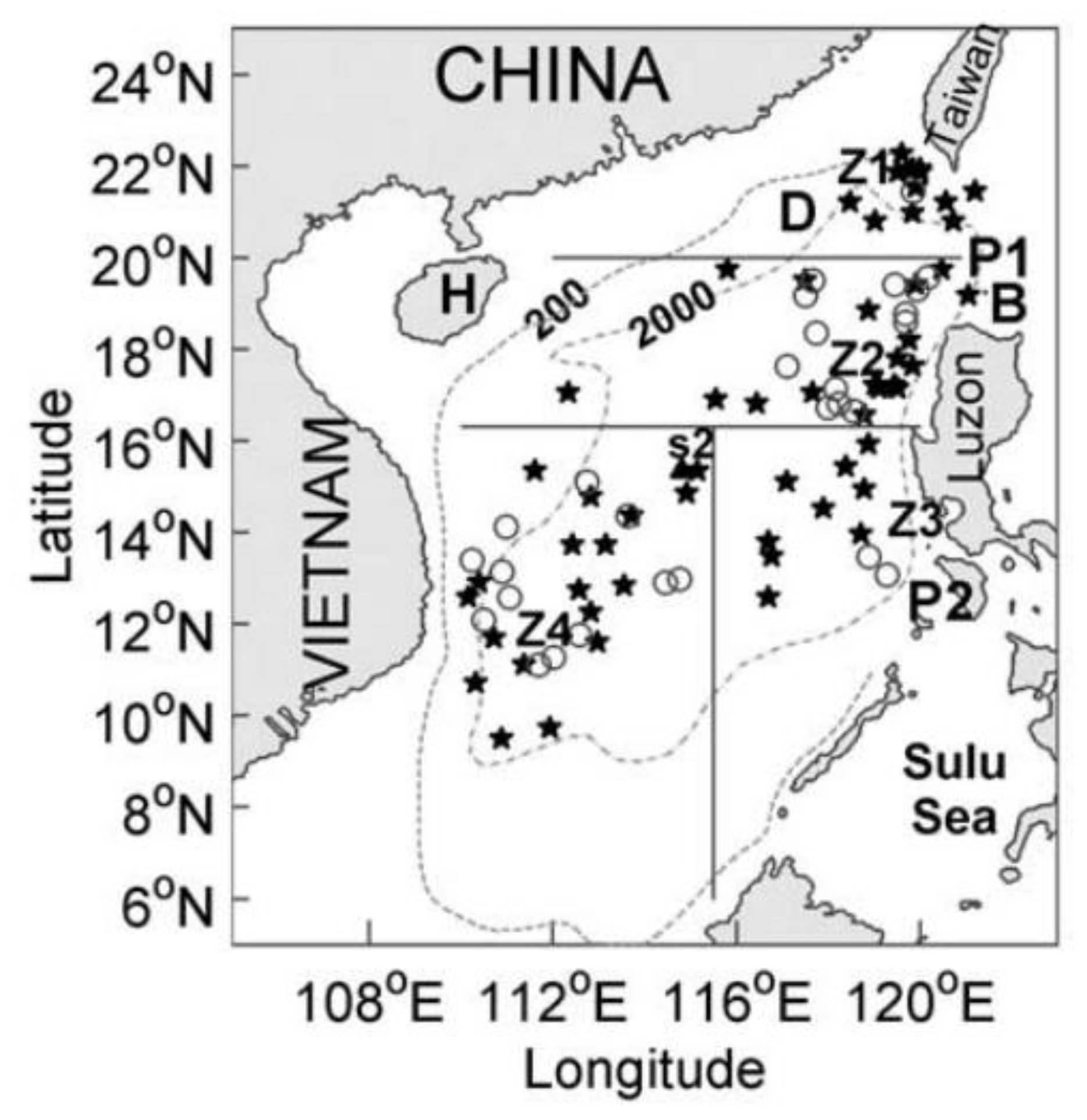
3.1. Datasets

We utilized the GSMCT, HD, and DTW methods to examine the complex trajectories of the mesoscale eddies in the SCS. The mesoscale ocean eddies were first identified from the Sea Level Anomaly (SLA) dataset, which has a daily temporal resolution and a ¼ degree spatial resolution, and is widely used in studying mesoscale ocean eddies [37]. We developed and improved the eddy tracking methods to reconstruct the complex trajectories of the mesoscale eddies in the SCS, and the results were thoroughly verified by our research group [28,38,39]. Previous studies have shown that the mesoscale eddies in the SCS usually have a life span of 28 days or more [26]. As a result, all complex trajectories examined in this study span 28 days or more. Among them, there were 626 and 730 complex trajectories derived from anticyclonic eddies (AEs) and cyclonic eddies (CEs), respectively. The two types (AEs and CEs) of ocean eddies are different in terms of the water rotation directions and the temperature gradient. Water in an AE rotates clockwise in the Northern Hemisphere and the temperature at its center is higher than the flange. By contrast, water in a CE rotates counterclockwise in the Northern Hemisphere, and the temperature is lower at the center than that around it [26]. Previous studies have shown that these two types of eddies have their own migration patterns. Their influences on energy and heat transfer are also substantially different. In oceanography, it is a common practice to examine AE and CE separately, just as we did in this study.

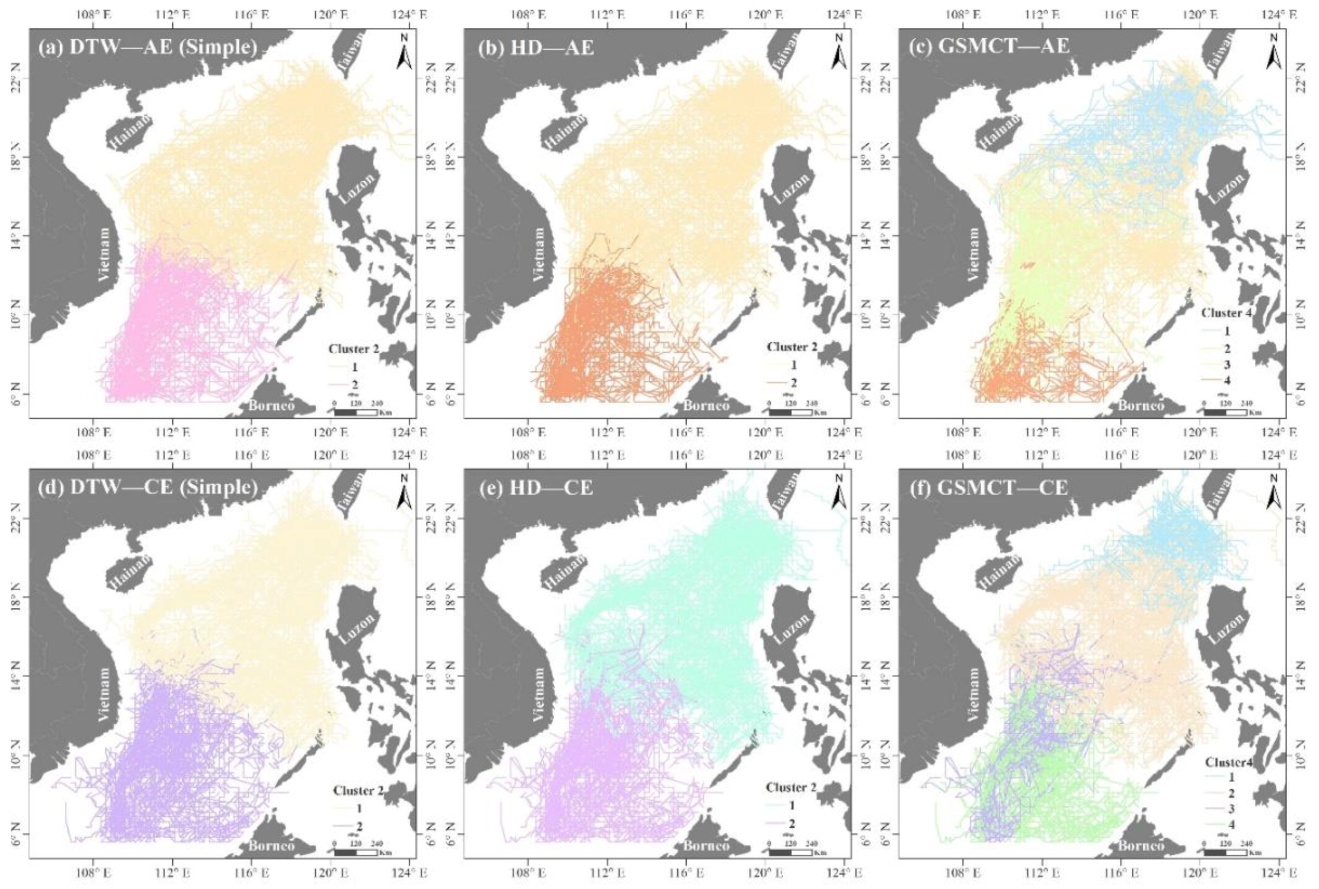
3.2. Clustering Results and Comparisons

The highest Calinski–Harabaz Index was found when the trajectories were grouped into four clusters using GSMCT, and two clusters using the HD and DTW methods, respectively (Figure 4a). The hierarchical clustering trees of the AEs an CEs generated by the GSMCT method are shown in Figure 4b,c with the red lines cutting the trajectories into four clusters. The clustering trees and cutting lines of the HD and DTW methods are not shown in this paper.

Figure 5 shows the clustered results of the AE and CE complex trajectories based on the similarity results derived from the DTW, the HD, and the GSMCT methods, respectively. The former two methods both clustered the AE and CE trajectories into two very similar groups roughly along a diagonal between the 12° and 14° parallels, respectively (Figure 5a,b,d,e). Both the AE and CE complex trajectories are grouped into four categories based on the global similarity calculated using the GSMCT method (Figure 5c,f).

Table 1. Statistics of the spatial proximity and structural similarity between and within the clusters.

Methods	Clusters	Anticyclonic Eddies (AEs) (Mean ± Standard Deviation)		Cyclonic Eddies (CEs) (Mean ± Standard Deviation)
		Spatial Proximity	Topologic Similarity	Spatial Proximity	Topologic Similarity
DTW	Cluster 1	0.73 ± 0.12	—	0.76 ± 0.11	—
	Cluster 2	0.80 ± 0.09	—	0.82 ± 0.08	—
HD	Cluster 1	0.70 ± 0.12	0.40 ± 0.20	0.73 ± 0.11	0.41 ± 0.18
	Cluster 2	0.82 ± 0.07	0.39 ± 0.19	0.79 ± 0.08	0.40 ± 0.20
GSMCT	Cluster 1	0.79 ± 0.08	0.60 ± 0.10	0.73 ± 0.12	0.57 ± 0.12
	Cluster 2	0.71 ± 0.12	0.56 ± 0.12	0.83 ± 0.07	0.56 ± 0.11
	Cluster 3	0.85 ± 0.07	0.55 ± 0.11	0.75 ± 0.10	0.62 ± 0.10
	Cluster 4	0.74 ± 0.11	0.59 ± 0.08	0.84 ± 0.07	0.59 ± 0.09

shows the statistics of the spatial and topologic similarity of the clusters identified. Overall, the average of the spatial proximity of the clusters generated by all three methods is very similar and within a range from 0.70 to 0.84, regardless of the type of ocean eddy. By contrast, the average topologic similarity of the clusters generated by the GSMCT method is around 0.6, which is higher than that of the clusters generated by the HD method. In other words, the GSMCT method is able to group trajectories with more similar topologic structures.

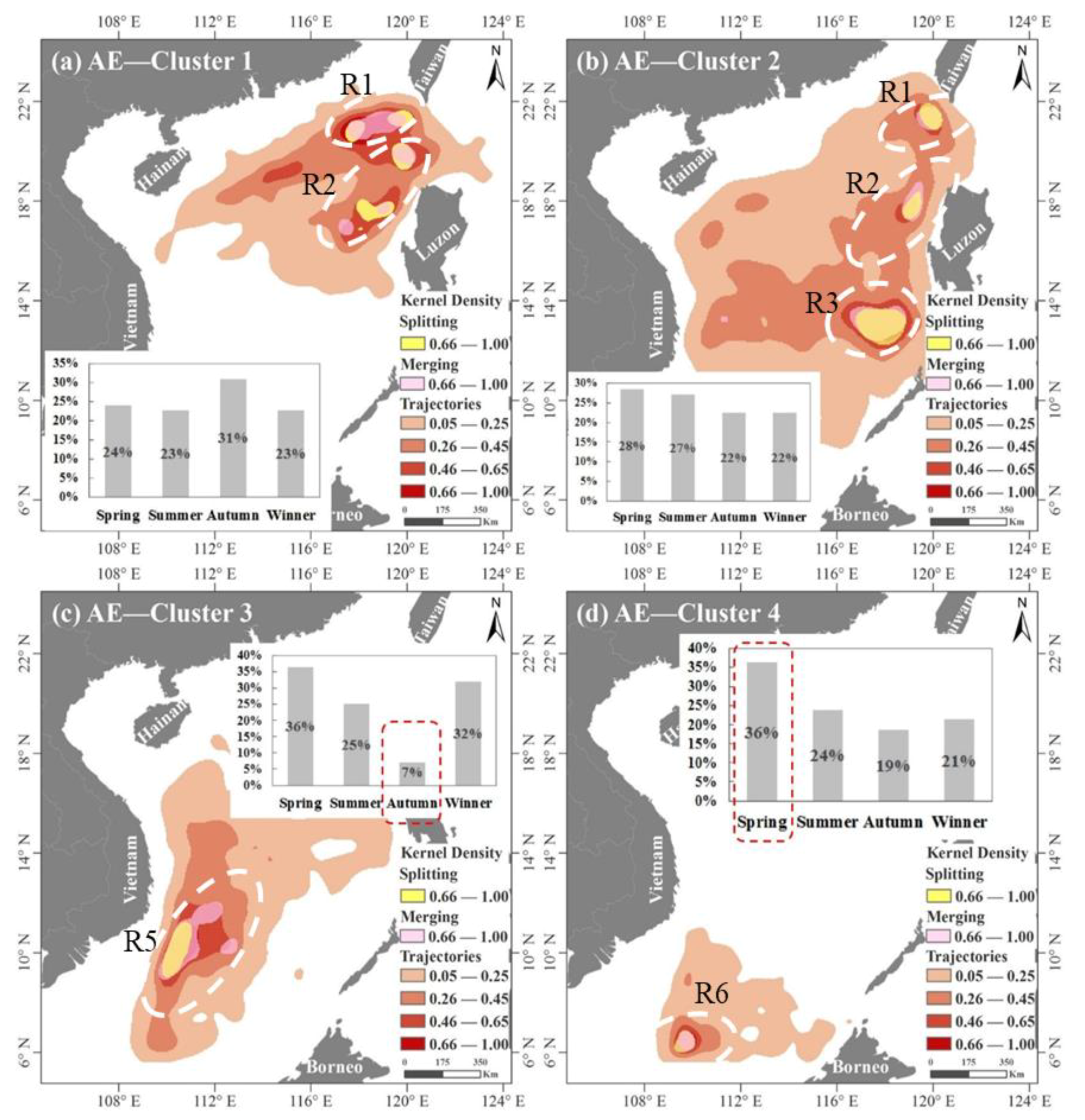
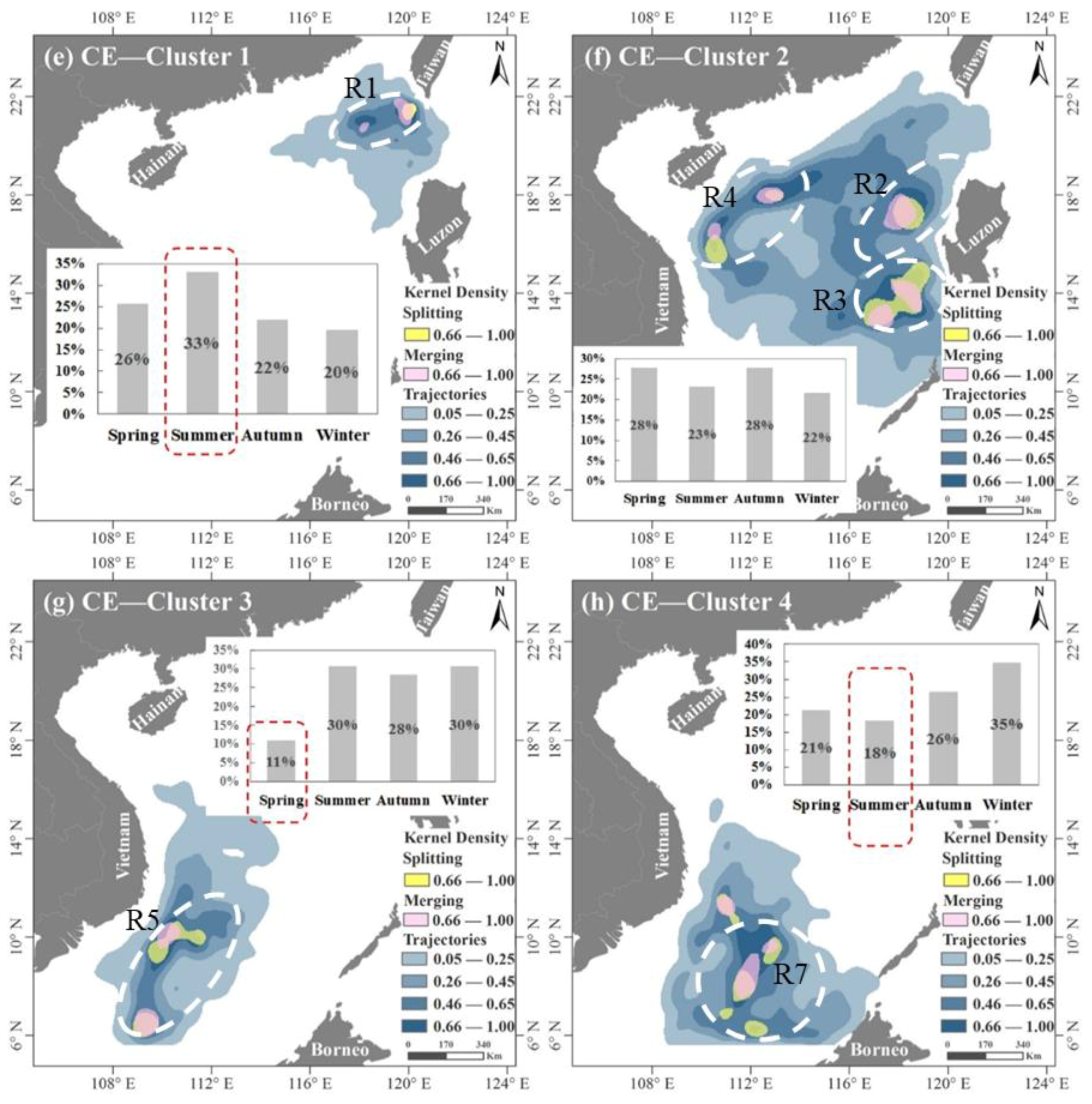
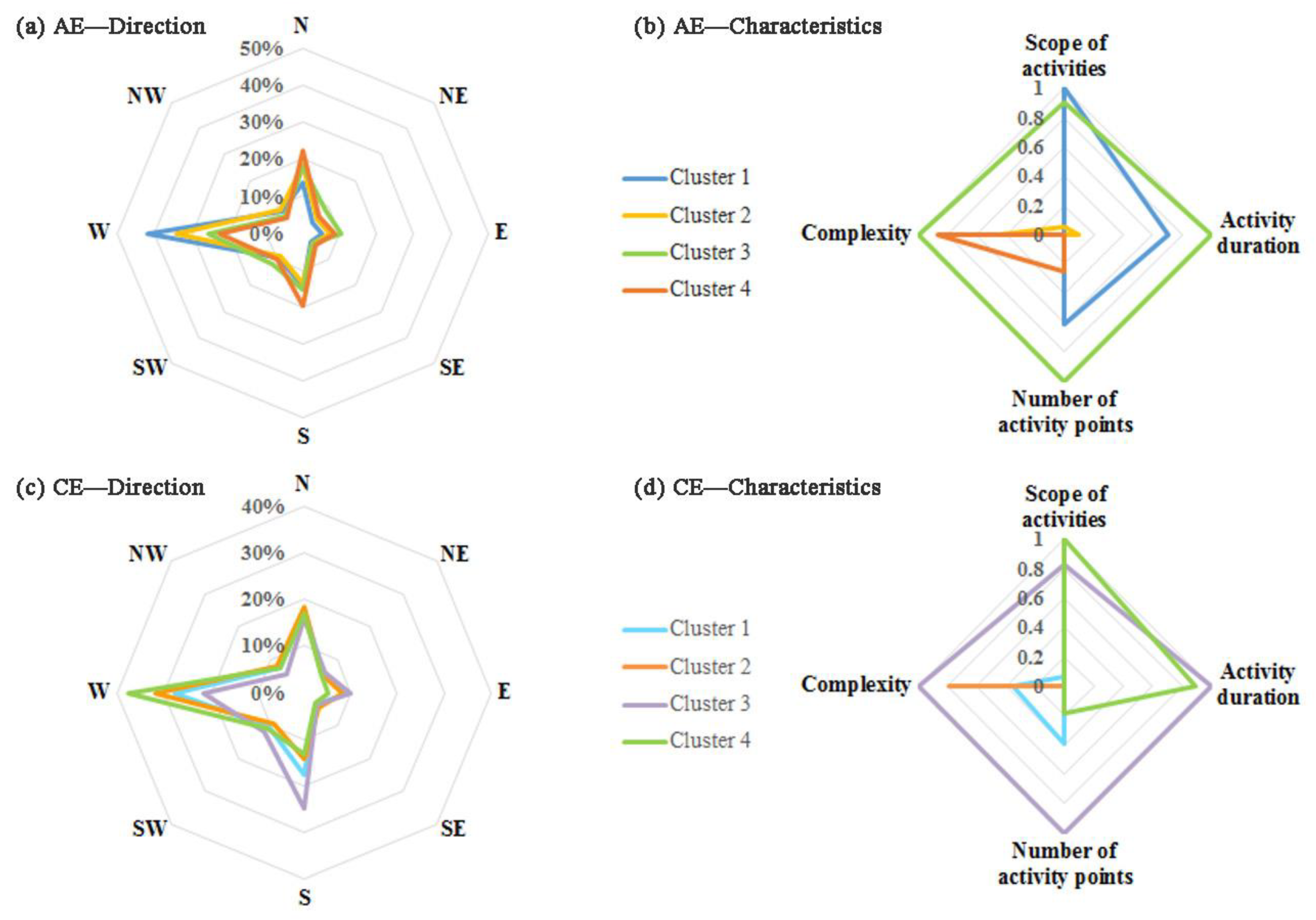
3.3. Spatio-Temporal Characteristics

Figure 6 shows the annual variations in the numbers of AE and CE complex trajectories in each cluster across the SCS. The total numbers of the AE complex trajectories from 1993 to 2016 in the four clusters are 84, 385, 44, and 113, respectively. By contrast, the total numbers of the CE complex trajectories in the four clusters are 133, 418, 46, and 133, respectively. The yearly numbers of AE and CE complex trajectories vary most significantly in the clusters located in the central SCS (Figure 5c,f), indicating that the variation of various environmental factors in the central SCS is relatively large, which leads to the instability of eddy property.

Figure 7 shows the kernel density of all complex trajectories, the seasonal variations in the number of complex trajectories, and the merging and splitting activities of the AE and CE complex trajectories. In this study, the seasons of spring, summer, autumn, and winter are the periods from March to May, from June to August, from September to November, and from December to February, respectively [26]. Spatially, the clusters of AE and CE complex trajectories are very consistent (Figure 7). The two smaller clusters of both AE and CE trajectories, Clusters 1 and 4, are located in the northernmost and southernmost of the SCS, respectively. The largest cluster, Cluster 2, is mainly located in the central SCS. Cluster 3 is located along the Vietnam offshore in the southwestern SCS.

High trajectory density within the clusters is mainly located in the places where mesoscale ocean eddies are born, or around the channels through which the eddies migrate, including the southwest of Taiwan Island (Figure 7a,e—R1) within Cluster 1, the west/southwest of Luzon Island (Figure 7b,f—R2,R3) and the continental shelf of the northern SCS (Figure 7f—R4) within Cluster 2, along the Vietnam offshore (Figure 7c,g—R5) within Cluster 3, and the southernmost of the SCS (Figure 7d—R6, Figure 7h—R7) within Cluster 4. Almost all regions (R1, R2, R3, R5, R6, and R7) with dense trajectories are located within the places where most eddies are born, as shown in previous studies [26,29,40]. It has been well documented that the factors contributing to eddy genesis vary significantly across the SCS, including the local wind stress in the southwest of Taiwan Island [26], the invasion of Kuroshio into the Luzon Strait [29], the variations in strong wind stress curl in the southwest of Luzon Island [26], and the instability of eastward jet in the Vietnam offshore [40]. It is worthy to note that region R4 within Cluster 2 is the most prominent migration channel in the SCS, through which most mesoscale ocean eddies propagate southwestward along the continental shelf until they reach the water in the southeast of Hainan Island [26].

The seasonal variations in the numbers of complex trajectories within the clusters are different across the SCS. For example, the AE complex trajectories of Cluster 1 are mainly found in autumn (Figure 7a), whereas those of the Cluster 4 are in spring (Figure 7d). The CE complex trajectories of Cluster 1 occur more in summer and less in winter (Figure 7e). By contrast, the CE complex trajectories of Cluster 4 occur more in winter and less in summer (Figure 7h).

The branch nodes (i.e., where the splitting and merging activities occur) along the complex trajectories are also mainly found in the places where most eddies are born or migrate through. Such places include the southwest of Taiwan Island (R1), the northwest and southwest of Luzon Island (R2, R3), and the southeast of Vietnam (R5). When mesoscale ocean eddies migrate through their major migration corridors, the intra-eddy interaction intensifies and, subsequently, eddies tend to split and/or merge more [41]. New eddies can also be generated as a result of the splitting or merging processes [42]. The intra-eddy interaction, thus the splitting and merging processes, could be attributed to wind stress and the Kuroshio intrusion in the southwest of Taiwan Island (R1) [26,29], the wind stress curl formed by the interaction between wind and topography in the northwest and southwest of Luzon Island (R2, R3) [42], and the strong eastward jet shooting away from the coast in the southeast of Vietnam (R5) [40]. The strong eastward jet may also significantly interrupt the movement of the water masses in the southeast of Vietnam, and forces more eddies to either merge or split. It is worthy to note that eddy splitting and merging activities were mainly found in the same places across the SCS.

3.4. Migration Characteristics

We further analyzed the moving direction, activity scope, activity duration, number of activity points, and the complexity of the AE and CE complex trajectories within each cluster. The moving direction refers to the major migration orientation and is determined by summarizing the instantaneous movement directions (North (N), Northeast (NE), East (E), Southeast (SE), South (S), Southwest (SW), West (W), Northwest (NW)) of the trajectory points. The activity scope is defined as the maximum distance between any two points along a specific trajectory, indicating the maximum spatial span within which an eddy is moving around. The activity duration refers to the lifespan of an eddy, indicating how long an eddy process could last. The number of activity points refers to the daily total number of points. More activity points suggests a more active eddy process. The complexity has been defined in Section 2.1 and it shows how complex an eddy′s topologic structure can be.

Figure 8 shows the dominant moving directions and the dynamic characteristics of the AE and CE complex trajectories. Both AE and CE show an obvious westward migration trend across the whole SCS, and a slightly north–south movement trend in the northern and central SCS (AE—Cluster 1, CE—Cluster 2) and the central part of the SCS (AE—Cluster 2, CE—Cluster 2). The westward movement trend could be attributed to the beta effect, whereas the longitudinal movement to the uneven Coriolis forces [39]. However, the AE and CE in the southern SCS (AE—Cluster 3, AE—Cluster 4, CE—Cluster 3, CE—Cluster 4), particularly those in the southeast of Vietnam offshore (AE—Cluster 3, CE—Cluster 3), mainly move toward west, north, and south. The instability of Vietnam′s offshore current affected by wind stress vorticity drives the eddies here to move north–south along the oscillation of Vietnam′s offshore current [40].

The trajectory clusters in the southeastern offshore of Vietnam (AE—Cluster 3 and CE—Cluster 3) include fewer trajectories (44 and 46 trajectories, respectively (Figure 6)) than the other clusters. However, the trajectories within these two clusters have the largest activity scope (606 km, 488 km), the longest activity cycle (124 days, 126 days), the largest daily number of activity points (1, 1), and the highest complexity (0.56, 0.52). This may show that the unstable conditions in southeastern Vietnam may drive the eddies here migrate more actively and split/merge more frequently. The AE—Cluster 2 and CE—Cluster 2 in the central SCS have 385 and 428 trajectories (Figure 6), respectively. By contrast, the complex trajectories in these two clusters have the smallest activity scope (234 km, 218 km), the shortest activity cycle (56 days, 50 days), and the fewest daily number of activity points (0.25, 0.32).

The AE and CE complex trajectories within the clusters in the northernmost (AE—Cluster 1 and CE—Cluster 1) and southernmost (AE—Cluster 4 and CE—Cluster 4) regions of the SCS show opposite activity patterns. The AE in Cluster 1 (shown in blue in Figure 8b) has a wider activity scope (606 km, 209 km), a longer activity period (124 days, 47 days), and a larger daily number of activity points (0.61, 0.25) than those in Cluster 4 (orange). By contrast, the AE complex trajectories in Cluster 4 have a higher complexity (0.53, 0.38) than those in Cluster 1 (orange). The CE complex trajectories in Cluster 4 (green in Figure 8d) have a wider range of activities (548 km, 228 km), a longer activity cycle (118 days, 50 days), and more daily activity points (0.40, 0.18) than those in Cluster 1 (blue), though the complexity of the CE complex trajectories in Cluster 1 (0.48) is higher than those of Cluster 4 (0.37).

4. Discussion

The aforementioned results show the advantages of the GSMCT algorithm in unraveling the spatial aggregation patterns of complex trajectories in the SCS. Some of the aggregation patterns identified in this study are consistent with those reported in previous studies, indicating the usefulness of GSMCT in studying the complex trajectories of mesoscale eddies in the SCS. For example, Wang et al. [43] divided the SCS into four zones based on the different mechanisms of eddy generation: Z1 in the southwest of Taiwan Island, Z2 in the northwest of Luzon Island, Z3 in the southwest of Luzon Island, and Z4 in the offshore of Vietnam (Figure 9). The zoning boundaries are generally similar to those identified in this study (Figure 4c,f and Figure 9). GSMCT clustered both the AE and CE complex trajectories in the SCS into four spatial zones: The northwest and southwest of Taiwan Island (Cluster 1), the central SCS (Cluster 2), the southeast of Vietnam (Cluster 3), and the southernmost SCS (Cluster 4). Within these four clusters, more trajectories are mainly found around the places where most eddies are born or migrate through [26,29,40]. The places with intense splitting and merging activities, regardless of AE or CE, are consistent and mainly located in the regions where mesoscale eddies are frequently born. This indicates that the topologic structures of the complex trajectories formed by eddy splitting or merging are probably related to the mechanisms that contribute to eddy formation in the SCS.

Differences do exist between our study and Wang et al. The Z2 and Z3 zones in Wang et al. [43] are combined into the same cluster (Cluster 2 in this study). Moreover, we identified one more cluster (Cluster 4) in the southernmost SCS from Z3 in [43]. The difference may be due to the different datasets that were used in the studies. Eddies with a life cycle over 60 days were considered in Wang et al. By contrast, this study only includes the complex trajectories that last 28 days or more. Most previous studies utilized the datasets with a weekly temporal resolution [26,43,44] and from such datasets the daily splitting and merging events could not be captured. The dataset we used in this study has a daily spatial resolution, which allows more splitting and merging events to be identified.

This study also added new knowledge to the oceanography field. For AE and CE complex trajectories, Cluster 1 in the northernmost and Cluster 4 in the southernmost SCS have the same number of complex trajectories. However, the complex trajectories show totally opposite seasonal variation and motion patterns. The AE complex trajectories within Cluster 1 are mainly found in autumn (Figure 7a), whereas the AE complex trajectories within Cluster 4 in spring (Figure 7d). The complex trajectories within Cluster 1 (blue) show a wider activity scope, a longer activity period, and a larger number of daily activity points than those in Cluster 4 (orange). However, the complex trajectories in Cluster 4 have a higher complexity than those in Cluster 1 (Figure 8b). More CE complex trajectories in Cluster 1 occur in summer and fewer in winter (Figure 7e). By contrast, those in Cluster 4 more occur in winter and less in summer (Figure 7h). The complex trajectories within Cluster 4 (green) have a wider activity scope, a longer life span, and more daily activity points than those in Cluster 1 (blue). However, the complexity of the complex trajectories in Cluster 1 is higher than that of the Cluster 4 (Figure 8d). Such an opposite pattern of the complex trajectories in the northernmost and southernmost SCS may be due to the regional variations in monsoon climate, topography, and Kuroshio, though further studies are needed. This study also shows that the mesoscale ocean eddies are more dynamic in the southeastern Vietnam offshore. The AE and CE complex trajectories in the southeastern Vietnam offshore (Cluster 3) have the longest activity cycle, the widest activity range, and the highest complexity.

It is worth noting that in our practical application, the importance of topological similarity and spatial proximity is the same in Equation (5), α = β = 1/2 (α represents the weight of topological structure similarity, β represents the weight of spatial proximity). We further discussed the other two cases to compare and analyze the influence of different weights on the clustering results of AE and CE complex trajectories. One case is that the weight of topological similarity is less than that of spatial proximity (α = 1/3, β = 2/3), Another case is that the weight of topological similarity is greater than that of spatial proximity (α = 2/3, β = 1/3). The results are shown in Figure 10; it can be seen that when the weight of spatial proximity is greater than the topological similarity, its highest Calinski–Harabaz Index is the largest of the three cases, indicating that the clustering is better, which is because the trajectories themselves gather in space. When the weight of topological similarity is greater than the spatial proximity, its highest Calinski–Harabaz Index is the smallest of the three cases, which shows that clustering results focusing on topological similarity are not as good as spatial proximity. Therefore, the change of different weights affects the clustering effect. When using this method, we can adjust the weights according to the data or the actual application needs.

Though some findings are consistent with previous research and new knowledge was generated in this study, there is still room for improvement of the GSMCT method. GSMCT clusters the complex trajectories based on their spatial proximity and topologic similarity without integration of any physical attributes of the points, i.e., the physical characteristics of the eddies. Our future work will expand and improve the GSMCT method by incorporating the physical characteristics of the ocean eddies to better cluster their complex trajectories. It is also already on our agenda to apply our GSMCT method to study other dynamic features and explore how different weight assignments in Equation (5) affect trajectory clustering.

5. Conclusions

We proposed a new method, GSMCT, to examine the similarity of complex trajectories in terms of their topological structure and spatial proximity. The similarity evaluation results were then used to cluster and examine the spatial patterns of the trajectories. We then utilized the method to examine the complex trajectories of the mesoscale ocean eddies in the SCS from 1993 to 2016 and four clusters were identified. Results show that regions with high trajectory density and intense splitting and merging activities are mainly found around the places where most AE and CE are born or migrate through in the SCS. Our results also show that the AE and CE in the southeastern Vietnam offshore are more complicated in terms of their migration and dynamic characteristics than those in other regions of the SCS.

This study finds one cluster in the northernmost and another one in the southernmost SCS. The numbers of the complex trajectories in these two clusters are almost the same. However, these two clusters exhibit significantly opposite patterns in terms of their seasonal variations in the eddy numbers and movement characteristics, probably indicating that the evolutions of eddies in these two regions are controlled by different factors or same factors in a totally opposite way. Such findings could help us better understand the relevant complex oceanographic processes, as well as their impacts on the salt and heat transport and consequently other marine biologic and biogeochemistry processes in these two regions. It also could provide some essential data for eddy simulation studies in these two areas.

References

1. Miller, H.J.; Han, J. Geographic Data Mining and Knowledge Discovery; CRC press: Boca Raton, FL, USA, 2001; pp. 352–366. [Google Scholar]
2. Zheng, Y. Trajectory Data Mining: An Overview; ACM: New York, NY, USA, 2015; pp. 1–14. [Google Scholar]
3. Yuan, G.; Sun, P.; Zhao, J. A review of moving object trajectory clustering algorithms. Artif. Intell. Rev. 2017, 47, 123–144. [Google Scholar] [CrossRef]
4. UrKa, D.; Kevin, B.; Francesca, C. Analysis and visualisation of movement: An interdisciplinary review. Mov. Ecol. 2015, 3, 5. [Google Scholar]
5. Wang, H.M.; Du, Y.; Yi, J. A new method for measuring topological structure similarity between complex trajectories. IEEE Trans. Knowl. Data Eng. 2019, 31, 1836–1848. [Google Scholar] [CrossRef]
6. Chen, J.; Wang, R.; Liu, L. Clustering of trajectories based on Hausdorff distance. In Proceedings of the IEEE International Conference on Electronics, Communications and Control, Ningbo, China, 9–11 September 2011; pp. 1940–1944. [Google Scholar]
7. Atev, S.; Miller, G.; Papanikolopoulos, N.P. Clustering of vehicle trajectories. IEEE Trans. Intell. Transp. Syst. 2010, 11, 647–657. [Google Scholar] [CrossRef]
8. Dodge, S.; Laube, P.; Weibel, R. Movement similarity assessment using symbolic representation of trajectories. Int. J. Geogr. Inf. Sci. 2012, 26, 1563–1588. [Google Scholar] [CrossRef] [Green Version]
9. Besse, P.; Guillouet, B.; Loubes, J.M. Review & Perspective for distance based clustering of vehicle trajectories. IEEE Trans. Intell. Transp. Syst. 2016, 17, 3306–3317. [Google Scholar]
10. You, W.; Chenghu, Z.; Tao, P. Semantic-geographic trajectory pattern mining based on a new similarity measurement. ISPRS Int. J. Geo-Inf. 2017, 6, 212. [Google Scholar]
11. Qiu, X.; Mao, Q.; Tang, Y. Reversed graph embedding resolves complex single-cell trajectories. Nat. Methods 2017, 14, 979–982. [Google Scholar] [CrossRef] [Green Version]
12. Gudmundsson, J.; Laube, P.; Wolle, T. Computational movement analysis. In Springer Handbook of Geographic Information; Springer: Berlin, Germany, 2012; Volume 112, pp. 423–438. [Google Scholar]
13. Nan, F.; He, Z.; Zhou, H.; Wang, D. Three long-lived anticyclonic eddies in the northern South China Sea. J. Geo-Phys. Res. Ocean. 2011, 116, 879–889. [Google Scholar] [CrossRef]
14. Liu, W.; Li, X.; Rahn, D.A. Storm Event Representation and Analysis Based on A Directed Spatiotemporal Graph Model; Taylor &Francis Group: London, UK, 2016; pp. 1–14. [Google Scholar]
15. Günther, G.; Müller, R.; Von Hobe, M. Quantification of transport across the boundary of the lower stratospheric vortex during Arctic winter 2002/2003. Atmos. Chem. Phys. 2008, 8, 3655–3670. [Google Scholar] [CrossRef] [Green Version]
16. Magdy, N.; Sakr, M.A.; Abdelkader, T.M. Review on trajectory similarity measures. In Proceedings of the 2015 IEEE Seventh International Conference on Intelligent Computing and Information Systems (ICICIS), Cairo, Egypt, 12–14 December 2015. [Google Scholar]
17. Alt, H. The computational geometry of comparing shapes. In Efficient Algorithms; Lecture Notes in Computer Science; Springer: Berlin, Germany, 2009; Volume 5760, pp. 235–248. [Google Scholar]
18. Pelekis, N.; Andrienko, G.; Andrienko, N.; Kopanakis, I.; Marketos, G.; Theodoridis, Y. Visually exploring movement data via similarity-based analysis. J. Intell. Inf. Syst. 2012, 38, 343–391. [Google Scholar] [CrossRef]
19. Yuan, Y.; Raubal, M. Measuring similarity of mobile phone user trajectories–A spatio-temporal edit distance method. Int. J. Geogr. Inf. Sci. 2014, 28, 496–520. [Google Scholar] [CrossRef]
20. Vaughan, N.; Gabrys, B. Comparing and combining time series trajectories using dynamic time warping. Procedia Comput. Sci. 2016, 96, 465–474. [Google Scholar] [CrossRef] [Green Version]
21. Foggia, P.; Sansone, C.; Vento, M. A performance comparison of five algorithms for graph isomorphism. In Proceedings of the 3rd IAPR TC-15 Workshop on Graph-based Representations in Pattern Recognition, Napoli, Italy, 19–21 January 2001; pp. 188–199. [Google Scholar]
22. Cordella, L.P.; Foggia, P.; Sansone, C. A (sub)graph isomor-phism algorithm for matching large graphs. IEEE Trans. Pattern Anal. Mach. Intell. 2004, 26, 1367–1372. [Google Scholar] [CrossRef]
23. Yang, S.; Xing, J.; Chen, D. A modelling study of eddy-splitting by an Island/Seamount. Ocean Sci. 2017, 13, 1–25. [Google Scholar] [CrossRef] [Green Version]
24. Li, Q.Y.; Sun, L.; Lin, S.F. GEM: A dynamic tracking model for mesoscale eddies in the ocean. Ocean Sci. Discuss. 2016, 12, 1249–1267. [Google Scholar] [CrossRef] [Green Version]
25. Adams, D.K.; Mullineaux, L.S. Surface-generated mesoscale eddies transport deep-sea products from hydrothermal vents. Science 2011, 332, 580–583. [Google Scholar] [CrossRef] [Green Version]
26. Chen, G.; Hou, Y.; Chu, X. Mesoscale eddies in the South China Sea: Mean properties, spatiotemporal variability, and impact on thermohaline structure. J. Geophys. Res. 2011, 116, 1–20. [Google Scholar] [CrossRef]
27. Du, Y.; Yi, J.; Wu, D. Mesoscale oceanic eddies in the South China Sea from 1992 to 2012: Evolution processes and statistical analysis. Acta Oceanol. Sin. 2014, 33, 36–47. [Google Scholar] [CrossRef]
28. Yi, J.; Du, Y.; Liang, F. A representation framework for studying spatiotemporal changes and interactions of dynamic geographic phenomena. Int. J. Geogr. Inf. Sci. 2014, 28, 1010–1027. [Google Scholar] [CrossRef]
29. Zhang, Z.; Zhao, W.; Qiu, B. Anticyclonic eddy sheddings from Kuroshio loop and the accompanying cyclonic eddy in the northeastern South China Sea. J. Phys. Oceanogr. 2017, 47, 1243–1259. [Google Scholar] [CrossRef] [Green Version]
30. Yang, Y.; Wang, D.; Wang, Q. Eddy-induced transport of saline kuroshio water into the Northern South China Sea. J. Geophys. Res. Oceans 2019, 124. [Google Scholar] [CrossRef]
31. Du, Y.; Wu, D.; Liang, F. Major migration corridors of mesoscale ocean eddies in the South China Sea from 1992 to 2012. J. Mar. Syst. 2016, 158, 173–181. [Google Scholar] [CrossRef] [Green Version]
32. Calinski, T.; Harabasz, J. A dendrite method for cluster analysis. Commun. Stat. 1974, 3, 1–27. [Google Scholar]
33. Liu, X. Entropy, distance measure and similarity measure of fuzzy sets and their relations. Fuzzy Sets Syst. 1992, 52, 305–318. [Google Scholar]
34. Chen, S.; Ma, B.; Zhang, K. On the similarity metric and the distance metric. Theor. Comput. Sci. 2009, 410, 2365–2376. [Google Scholar] [CrossRef] [Green Version]
35. Miller, H.J.; Han, J. Geographic Data Mining and Knowledge Discovery, 2nd ed.; Taylor & Francis Group: London, UK, 2009. [Google Scholar]
36. Liu, Y.; Li, Z.; Xiong, H. Understanding and enhancement of internal clustering validation measures. IEEE Trans. Cybern. 2013, 43, 982–994. [Google Scholar]
37. Noce, S.; Collalti, A.; Valentini, R.; Santini, M. Hot spot maps of forest presence in the Mediterranean basin. Infor. Biogeosci. For. 2016, 9, 766–774. [Google Scholar] [CrossRef]
38. Yi, J.; Du, Y.; He, Z. Enhancing the accuracy of automatic eddy detection and the capability of recognizing the multi-core structures from maps of sea level anomaly. Ocean Sci. 2014, 10, 39–48. [Google Scholar] [CrossRef] [Green Version]
39. Yi, J.; Du, Y.; Liang, F. An auto-tracking algorithm for mesoscale eddies using global nearest neighbor filter. Limnol. Oceanogr. Methods 2017, 15, 276–290. [Google Scholar] [CrossRef]
40. Gan, J.; Qu, T. Coastal jet separation and associated flow variability in the southwest South China Sea. Deep Sea Res. Part I Oceanogr. Res. Pap. 2008, 55, 1–19. [Google Scholar] [CrossRef]
41. Cui, W.; Wang, W.; Zhang, J. Multicore structures and the splitting and merging of eddies in global oceans from satellite altimeter data. Ocean Sci. 2019, 15, 413–430. [Google Scholar] [CrossRef] [Green Version]
42. Wang, H.M.; Du, Y.; Liang, F.Y.; Sun, Y. A census of the 1993–2016 complex mesoscale eddy processes in the South China Sea. Water 2019, 11, 1208. [Google Scholar] [CrossRef] [Green Version]
43. Wang, G.; Su, J.; Chu, P.C. Mesoscale eddies in the South China Sea observed with altimeter data. Geophys. Res. Lett. 2003, 30, 2121. [Google Scholar] [CrossRef] [Green Version]
44. Nan, F.; Xue, H.; Yu, F. Kuroshio intrusion into the South China Sea: A review. Prog. Oceanogr. 2015, 137, 314–333. [Google Scholar] [CrossRef] [Green Version]
Figure 1. A simple trajectory (a) versus a complex trajectory (b).
Ijgi 08 00574 g001
Figure 2. A flow chart showing how the CSM algorithm evaluates the topologic similarity of complex trajectories, a, b and c are examples of graph isomorphism, subgraph isomorphism and partial isomorphism respectively.
Ijgi 08 00574 g002
Figure 3. Simplification of a complex trajectory (a) into multiple simple trajectories (a1a6).
Ijgi 08 00574 g003
Figure 4. Variations in the Calinski–Harabaz Index regarding the number of clusters (a), the clustering trees (b), and the cutting lines (c).
Ijgi 08 00574 g004
Figure 5. Clustering results of AE (ac) and CE complex trajectories (df) using the DTW, HD, and GSMCT methods.
Ijgi 08 00574 g005
Figure 6. Variations in the annual numbers of AE (a) and CE (b) complex trajectories in each cluster from 1993 to 2016.
Ijgi 08 00574 g006
Figure 7. Kernel density and seasonal statistics of AE (ad) and CE (eh) complex trajectories within the four clusters. The elliptic boxes indicate where the trajectories are densely clustered. The yellow and pink colors represent where splitting and merging activities mainly occur, respectively. The insets show the seasonal variations in the numbers of complex trajectories.
Ijgi 08 00574 g007aIjgi 08 00574 g007b
Figure 8. Normalized statistics of moving direction and activity characteristics of AE and CE complex trajectories within different clusters.
Ijgi 08 00574 g008
Figure 9. The four geographic zones of the South China Sea (SCS), identified by Wang et al., mainly according to eddy formation mechanisms. The circles and stars denote CEs and AEs, respectively.
Ijgi 08 00574 g009
Figure 10. Variations in the Calinski–Harabaz Index regarding the number of clusters based on different weights (the red dotted ellipse represents the highest Calinski–Harabaz Index, that is, the best clustering result).
Ijgi 08 00574 g010