Accumulative Errors Optimization for Visual Odometry of ORB-SLAM2 Based on RGB-D Cameras


1
School of Remote Sensing and Information Engineering, Wuhan University, Wuhan 430079, China
2
State Key Laboratory of Information Engineering in Surveying Mapping and Remote Sensing, Wuhan University, Wuhan 430079, China
*
Author to whom correspondence should be addressed.
ISPRS Int. J. Geo-Inf. 2019, 8(12), 581; https://0-doi-org.brum.beds.ac.uk/10.3390/ijgi8120581
Submission received: 1 November 2019
/
Revised: 2 December 2019
/
Accepted: 9 December 2019
/
Published: 11 December 2019
(This article belongs to the Special Issue 3D Indoor Mapping and Modelling)
Abstract
:Oriented feature from the accelerated segment test (oFAST) and rotated binary robust independent elementary features (rBRIEF) SLAM2 (ORB-SLAM2) represent a recognized complete visual simultaneous location and mapping (SLAM) framework with visual odometry as one of its core components. Given the accumulated error problem with RGB-Depth ORB-SLAM2 visual odometry, which causes a loss of camera tracking and trajectory drift, we created and implemented an improved visual odometry method to optimize the cumulative error. First, this paper proposes an adaptive threshold oFAST algorithm to extract feature points from images and rBRIEF is used to describe the feature points. Then, the fast library for approximate nearest neighbors strategy is used for image rough matching, the results of which are optimized by progressive sample consensus. The image matching precision is further improved by using an epipolar line constraint based on the essential matrix. Finally, the efficient Perspective-n-Point method is used to estimate the camera pose and a least-squares optimization problem is constructed to adjust the estimated value to obtain the final camera pose. The experimental results show that the proposed method has better robustness, higher image matching accuracy and more accurate determination of the camera motion trajectory.
1. Introduction
Oriented feature from the accelerated segment test (oFAST) and rotated binary robust independent elementary features (rBRIEF) simultaneous location and mapping 2 (ORB-SLAM2) [1,2,3,4] is a complete simultaneous location and mapping solution based on monocular, binocular and RGB-Depth (RGB-D) cameras. One of its contributions is to propose an efficient visual odometry (VO) method based on improved oriented feature from the accelerated segment test (FAST) and rotated BRIEF operators. The purpose of visual odometry as the front end of SLAM is to estimate the rough camera motion based on information from adjacent images and provide a good initial value for the back end of SLAM, which is one of the key visual SLAM research technologies. A complete visual odometry consists of three main parts: (1) image feature extraction and matching, mainly including image feature detection, description and matching; (2) mismatched points culling, which can help improve image feature matching accuracy; and (3) motion pose estimation and triangulation measurement. This technology is widely used in robotic autonomous positioning, virtual reality, augmented reality and autonomous driving. In visual SLAM, since RGB-D cameras can obtain RGB and depth images simultaneously, they have better for application scenarios than monocular and binocular cameras indoors, thus attracting many researchers and enterprises to conduct in-depth research and development. More low-cost and high-performance RGB-D cameras are being launched, further promoting the indoor application and development of RGB-D cameras [5,6,7]. However, as the application scenarios continue to increase, higher requirements are placed on visual odometry based on RGB-D cameras. At present, some problems exist with visual odometry based on the RGB-D camera, which can be improved using feature point extraction and matching, camera pose recovery and so on [8,9]. Visual odometry has been a research hotspot in the field of computer vision and image real-time processing. Researchers have committed to proposing a more accurate and robust visual odometry method but the existing visual odometry solution cannot meet the needs of increasingly complex application scenarios.
We mainly studied the problem of camera tracking loss and trajectory drift caused by the accumulated error of a visual odometer. Based on the ORB-SLAM2 framework, a new visual odometer scheme is proposed. Specifically, the main innovations of this paper are as follows. First, feature point extraction is performed using adaptive threshold-based oriented features from the accelerated segment test (AoFAST) algorithm to enhance the robustness of feature extraction. Second, the results of rough matching are optimized using the fast library for approximate nearest neighbors (FLANN) [10] algorithm with progressive sample consensus (PROSAC) [11] algorithm and epipolar line constraints based on the essential matrix, thus improving the accuracy. The camera pose obtained using the proposed scheme has better robustness and higher precision.
2. Related Work
Visual odometry technology has developed rapidly and many effective algorithms and strategies have emerged. Although the existing algorithms can produce good results under certain conditions, some key problems remain to be solved in the face of complex scenarios, especially in terms of accuracy and robustness. Considering these problems, on the basis of literature and research work, we mainly improve the visual odometry to produce a visual odometry scheme with higher precision and higher robustness [12].
Image feature extraction and description technology is the basis of visual odometry and is an independent research hotspot that can be applied to many fields. At present, many effective feature extraction and description methods are available, such as the scale invariant feature transform (SIFT) [13] algorithm, the speeded up robust features (SURF) [14] algorithm, the binary robust invariant scalable keypoints (BRISK) [15] algorithm and the oriented FAST and rotated BRIEF (ORB) [16] algorithm. Feature point matching establishes a reliable correspondence between the homonymic feature points. The selection of matching strategy directly affects the matching accuracy of the corresponding points [17,18]. A common matching method is the brute force matcher but it is slow, so some scholars introduced a faster method: fast library for approximate nearest neighbors (FLANN). These are the two most commonly used feature point matching methods in engineering applications. However, points in the results of these algorithms can be mismatched, which may seriously affect the success and accuracy of the camera pose calculation. To improve the accuracy of feature point matching, scholars have used various methods and strategies to eliminate wrong matching points. Random sample consensus (RANSAC) [19,20,21,22,23] is a simple and effective method that obtains an optimal model by randomly selecting a specified number of matching point pairs and rejects the mismatched points according to the calculated model. The RANSAC method can be used to calculate the fundamental matrix of the image pair, which can be used to constrain the epipolar line to produce a more ideal matching result. The method is well applied in many scenarios where high precision matching is required. After image matching, the pose relationship between adjacent images can be restored, that is, the rotation matrix and translation matrix between images can be calculated. In photogrammetry and computer vision, image pose recovery is mainly divided into three categories: (1) two-dimensional-two-dimensional (2D-2D), which uses two sets of 2D points to estimate camera motion through epipolar line constraint; (2) three-dimensional-three-dimensional (3D-3D), which generally uses the iterative closest point (ICP) [24] to calculate camera motion based on two sets of 3D points; and (3) 3D-2D, which estimates the motion of the camera using the Perspective-n-Point (PnP) [25] method according to the 3D points of the object and their projection positions in the camera and is one of the most important pose estimation methods that does not require the use of epipolar line constraint and can obtain better motion estimation in few matching points. 3D-2D is ideal for real-time mapping and modeling of RGB-D sensor indoors. However, 3D-2D has insufficient information use and is influenced by noise and mismatches, resulting in algorithm failure. Therefore, suppressing noise, improving matching accuracy and improving use of matching information are some of the solutions to improve camera pose recovery. Besides, to reduce drift in the trajectory, landmarks [26], multi constraint Kalman filter [27] and 3D models have been used. For example, reference [26] utilizes two calibrated cameras that form a stereo head. It minimizes the error associated with each pose computation by allowing matching and pose estimating over longer motion baselines. Reference [27] proposes a measurement model for omnidirectional visual-inertial odometry with visual and inertial sensors for indoor positioning. Reference [28] proposes a building information model (BIM) based visual tracking approach for indoor localization using a 3D building model. It can avoid the accumulation of localization errors. Reference [29] proposes an indoor localization improved by spatial context, which uses maps and spatial models to improve the localization by constraining location estimates in the navigable parts of indoor environments. Reference [30] conducts a survey on visual-based localization with heterogeneous data. It presents a survey about recent methods that localize a visual acquisition system according to a known environment. They are limited to fixed scenes, data and facilities but not applicable to all scenes. In recent years, there are some representative achievements in the research of visual odometer based on image matching. For example, the adaptive threshold selection strategy of reference [31] is to dynamically adjust the threshold within a given range by comparing the number of FAST feature points with the threshold in the current window. In this way, the visual odometry algorithm has the advantages of a constant stream of robust features and feature count is nearly constant. In reference [32], a simple proportional controller is used to choose the adaptive threshold for the FAST detector in visual odometry. They all made some improvements. These improved ideas are worth learning. To summarize, given the existing problems, and under the framework of the ORB-SLAM2 visual odometry, we introduce an adaptive threshold oFAST algorithm for feature extraction to enhance its robustness and stability. PROSAC [33,34,35] is used to optimize the matching results and the epipolar line constraint [36] based on the essential matrix is introduced to further improve the image matching accuracy to improve the success rate and accuracy of camera pose recovery, reduce the accumulated error of ORB-SLAM2 visual odometry and provide a more reliable camera pose for local optimization and global optimization.
3. Methodology
The RGB-D camera used in this study was pre-calibrated. In the process of feature point extraction, we propose an adaptive threshold oFAST algorithm (adaptive threshold oFAST, AoFAST) to extract feature points and apply the FLANN algorithm for feature point coarse matching. Then, the obtained matching sets of homonymous points are optimized by the PROSAC algorithm. To further improve the matching accuracy of homonymous feature points, the essential matrix is introduced to conduct epipolar line constraint to purify mismatched points. Finally, the efficient Perspective-n-Point (EPnP) method is used to estimate the camera pose. Next, we introduce the improved visual odometry method in detail and verify the effectiveness and superiority of this method through experiments. Figure 1 is the flow chart of our improved visual odometry.
3.1. Visual Odometry Algorithm in ORB-SLAM2
3.1.1. Feature Extraction and Description
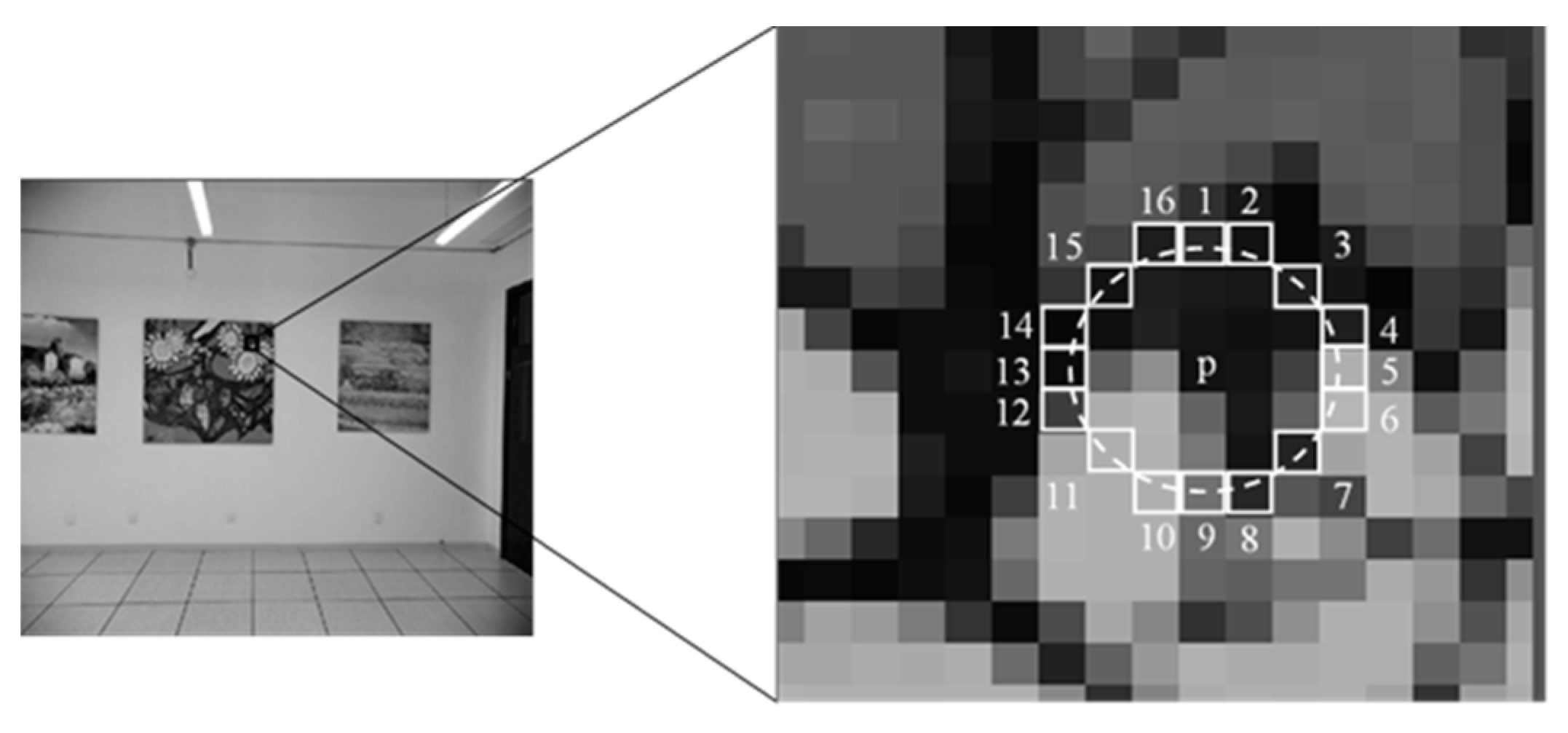
In ORB-SLAM2 visual odometry, feature point extraction uses the oFAST algorithm, which is an improvement of the traditional FAST algorithm. The traditional FAST algorithm functions by considering that if the gray value of a pixel differs considerably from the gray value of a certain number of pixels in its surrounding area, the pixel may be a corner point. To be more efficient, a pre-test operation can be added to quickly eliminate most pixels that are not corner points. As shown in Figure 2. The specific operation directly detects the gray value of the 1st, 5th, 9th and 13th pixels on the neighborhood circle for each pixel. Only when three of the four pixels are greater than or less than at the same time, the current pixel may be a corner point; otherwise, it should be directly excluded. is the gray value of the point to be detected and is the given threshold.
Compared to other corner detection algorithms, FAST only needs to compare the gray value of the pixels, so the algorithm is very fast. The main limitation of the FAST corner is the lack of directionality and scale invariance. To solve this problem, the visual odometry in ORB-SLAM2 improves upon the traditional FAST algorithm with the oFAST algorithm. In the oFAST algorithm, the directionality of features is realized using the gray centroid method and scale invariance is achieved by constructing an image pyramid and detecting corner points on each layer of the pyramid. FAST feature points have many extractions but poor stability but the extracted feature points have strong robustness. Therefore, the oFAST algorithm calculates the Harris response value for the original FAST corner points and then selects the corner points with larger response values as the final set of corner points. However, the oFAST algorithm uses a fixed threshold, which also makes it unable to meet the requirements of feature point extraction in complex scenes.
3.1.2. Image Matching and Error Elimination
A correct matching result is the goal of image matching. If mismatched feature point pairs are used to solve the polar geometry, large errors will be generated in the fundamental matrix obtained by the polar geometry, which considerably influences the positioning accuracy. Therefore, mismatched points culling is required after feature point extraction. In ORB-SLAM2 [2], the coarse-to-fine matching strategy of FLANN + RANSAC + fundamental matrix-based epipolar line constraint is used to achieve this goal. FLANN is a nearest neighbor search algorithm for large data sets and high-dimensional features that can quickly perform coarse matching on images from a large number of feature points. The RANSAC method is to randomly select some points as interior points in a set of sample points, including exterior points and interior points, to calculate the data model of the sample and ensure the data model generated by the selected sample points has good performance in the whole sample via iteration and threshold comparison. Most of the exterior points can be eliminated by the RANSAC method. However, due to the randomness of the initial sample selection of RANSAC, the running time of RANSAC is extremely unstable, therefore, a new algorithm is needed to solve these problems.
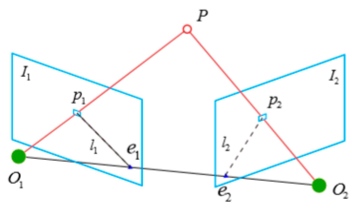
To further improve the accuracy of image matching, the epipolar line constraint is also used in ORB-SLAM2 to eliminate mismatched points. The epipolar line constraint means that a set of matching point pairs must be located above a corresponding set of epipolar lines on two images. As shown in Figure 3, is an image point in the left figure , is the corresponding image point in the right figure, is the object point corresponding to and and and are the photography centers of the left and right images, respectively. The intersection of the line with the image plane , is ,, which is the pole. ,, form an epipolar plane and the lines with which it intersects , are the epipolar lines. For the epipolar line constraint for each pixel on the left image, the corresponding homonymy point on the right image must be on the intersection line between the epipolar plane of the point and the right image (i.e., the core line). However, because the fundamental matrix introduces internal parameters, it also introduces more errors accordingly. Through the improvement of this point, better error purification effect can be achieved.
3.1.3. Pose Estimation
When restoring the pose relationship between images, the commonly used method is PnP. However, PnP cannot fully use information and is susceptible to noise and mismatching points. To solve these problems, a common method is using EPnP for pose solving as it can use more information and iteratively optimize the camera’s pose to eliminate the influence of noise as much as possible. In the ORB-SLAM2 visual odometry scheme, the EPnP algorithm is used to solve the camera pose and the improved visual odometry scheme proposed in this paper also uses this algorithm.
3.2. Improved Visual Odometry Algorithm for ORB-SLAM2
Generally, even in the same image, due to the uncertainty and complexity of illumination and surrounding environment information, problems may occur such as low contrast or strong local features. When the oFAST operator detects the corner points, the threshold value is fixed. If the threshold value is too low, many virtual corner points appear, thereby reducing the detection efficiency; if the threshold is too high, a certain degree of missed detection occurs. Although the fixed threshold is simple to calculate, it cannot meet the requirements of feature point extraction in different images. Secondly, in the process of removing the mismatched points, since the initial sample selected by RANSAC is completely random, RANSAC is prevented from selecting the interior point set that meets the model requirement at one time, making the number of iterations large and unstable. Consequently, the algorithm is slow. Due to the introduction of camera internal parameters, the epipolar line constraint based on fundamental matrix adopted by ORB-SLAM2 also introduces new errors and the calculation process is more complex. To solve these problems above, we improved the visual odometry of ORB-SLAM2. The first step is to select the threshold of the oFAST feature detection algorithm with an adaptive strategy, namely the AoFAST algorithm, which makes feature points extraction more robust in more complex environments. Afterwards, the initial sample selection method of RANSAC is improved to quickly obtain a relatively stable result. The fundamental matrix is replaced with an essential matrix to perform the epipolar line constraint, thus realizing a visual odometry with higher precision.
3.2.1. Adaptive Threshold oFAST Algorithm for Feature Extraction Algorithm
In the oFAST feature extraction, the selection of the threshold directly affects the effect of the corner points extraction and the number of corner points changes with the threshold. The fixed threshold is simple to calculate but lacks flexibility, complicating the extraction of satisfactory corner points. Therefore, we used an adaptive method to determine the threshold. In detail, we extracted feature points by setting the dynamic global threshold and the dynamic local threshold .
For setting dynamic global threshold , the optimal histogram entropy method, which was proposed by Kapur, Sahoo and Wong (KSW entropy method) [37] is adopted. In this method, the gray histogram of the image is used as an approximate estimation of the probability distribution density function of the gray value and then the objective function is constructed using the density function combined with the principle of entropy to select the threshold value.
Let the threshold divide the image with the gray range into two types of and . and are the pixel frequency distributions of and respectively. That is, and , where is the probability of each gray level. Set . and are the entropies of the two types, whereas is the entropy of the image. The values of , and are
and are the gray levels that maximize and minimize the entropy of the image, respectively; k is a coefficient, which is the same as in Equation (5). The dynamic global threshold can be expressed as
Since the KSW entropy method ignores the grayscale variation of the image locality, it cannot consider the effects of various changes, such as shadow, uneven illumination, burst noise and background abrupt changes. As such, it is necessary to further judge and screen the candidate feature points obtained using dynamic global thresholds. In this paper, the candidate feature points are further filtered by setting the dynamic local threshold .
Assume that the point in the image is the candidate feature point. Take as the center and take the side length of the rectangle as , define the dynamic local threshold as
where , represent the largest and the smallest gray value in the rectangular area , respectively; represents the average gray value in the rectangular area ; and is the coefficient.
3.2.2. New Image Matching Algorithm
FLANN is a good image rough matching method. In the coarse-to-fine image matching strategy in this paper, FLANN is used for image rough matching. In the fine matching phase, PROSAC and the epipolar line constraint based on essential matrix are used to obtain the final matching results.
Compared with the RANSAC [18] algorithm, the PROSAC [1] algorithm ranks the points in the sample set in advance; the interior points that can estimate the correct model are ranked higher and the exterior points that hinder the model estimation are ranked lower. Then, select a high-level point set to estimate the model that can reduce the randomness of the sampling and improve the success rate of obtaining the correct model. As a result, the number of algorithm iterations decreases. Specifically, the PROSAC algorithm classifies the feature matching point pairs by introducing a quality factor and high-quality matching point pairs are used to obtain the homography matrix [38].
In the image matching process, each pair of matching feature points produces a ratio of Euclidean distance. Equation (6) is the definition of , which is a ratio of two Euclidean distances. is the minimum Euclidean distance and is the sub minimum Euclidean distance.
The analysis shows that the smaller the values of and , the better the quality of the matching of feature points. Thus, PROSAC introduces a quality factor to measure the quality of the matching point pairs.
According to the analysis above, the larger the value of , the higher the relative probability that the matching point is an interior point or the higher the probability of obtained the correct model.
The specific steps of the PROSAC algorithm are shown in Algorithm 1.
| Algorithm 1. Progressive sample consensus (PROSAC) algorithm steps |
| Input: Maximum number of iterations , interior point error threshold and interior point number threshold Output: Homography matrix |
|
After the above processing, the proposed approach produces a more accurate matching point set and homography matrix. Thus, the fundamental matrix and the essential matrix can be calculated, both of which can be used to realize the epipolar line constraint to purify the set of matching points. The visual odometry of ORB-SLAM2 uses the epipolar line constraint based on the fundamental matrix. The fundamental matrix is more complex than the essential matrix in which the internal parameters may introduce more errors and the elimination the mismatches may not be satisfactory. Therefore, the proposed algorithm uses a simpler essential matrix to perform the epipolar line constraint, which is easier to calculate and the elimination the wrong matching point pairs is improved, so that a more accurate matching point set can be obtained, which is conducive to calculating a more accurate camera pose.
From Figure 3 above, assume that the coordinates of the object point are
According to the pinhole camera model, the pixel positions of the two pixel points and are shown in Equation (9), where is the camera internal parameter matrix and and are the camera motion rotation matrix and translation matrix, respectively.
Assume that , are the coordinates of the pixel on the normalized plane, which can be calculated by Equation (10):
Substitute Equation (10) into Equation (9):
Multiply Equation (11) by and simplify it, where is the antisymmetric matrix of .
where
The proposed method uses eight pairs of points to estimate the essential matrix. When considering a pair of matching points, their normalized coordinates are and . According to the epipolar line constraint, the Equation (14) can be obtained:
Eight pairs of matching points can realize eight equations and the linear equations composed of these eight equations can obtain the value of the essential matrix .
According to the definition of the essential matrix:
Equation (15) can be used to eliminate the mismatched point, where are a set of corresponding points on the two images.
3.2.3. Pose Estimation Algorithm
At present, the most commonly used camera pose recovery methods are PnP, EPnP [39], uncalibrated PnP (UPnP) [40] and the direct least-squares method for PnP (DLS) [41]. To compare the effectiveness and practicability of these methods, we conducted an experiment on the camera pose calculation of a pair of images and the experimental results are shown in Table 1.
From the experimental results, whether in terms of accuracy or time, EPnP provides more advantages than the other methods, so we chose EPnP method for camera pose estimation.
4. Experiments and Analysis
4.1. Experimental Data and Computing Environment
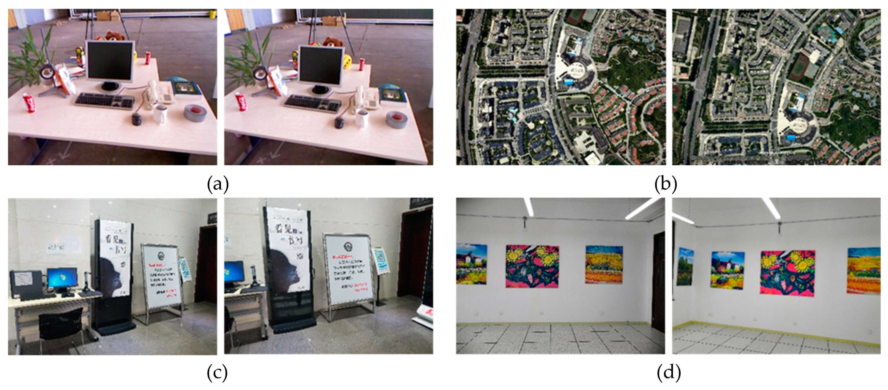
To verify the effectiveness of the proposed method, we used the proposed improved visual odometry method to conduct experiments and compared the experimental results with the results of the ORB-SLAM2 open source code. Since the improvement produced by this method only involves the visual odometry, the modules of loop detection and global optimization in ORB-SLAM2 are closed in the following experiments. In this study, we use Visual C++ based on OpenCV to program the proposed new method. In the experiment of the entire visual odometry, we used an Intel® Core™ i7-8750H processor and with 8 GB memory. We obtained video stream data from the open data set RGBD-Benchmark of the Technical University of Munich (TUM, Munich, Germany). The two video streams were rgbd_dataset_freiburg2_desk and rgbd_dataset_freiburg3_structure_texture_near. The track length of rgbd_dataset_freiburg2_desk is 18.880 m and the number of frames is 2964. For rgbd_dataset_freiburg3_structure_texture_near, the data are 5.050 m with 1065 frames. In the experiment comparison, the image pairs shown in Figure 4 were used.
4.2. Experimental Analysis
4.2.1. Experimental Results and Analysis of Image Feature Extraction Algorithm
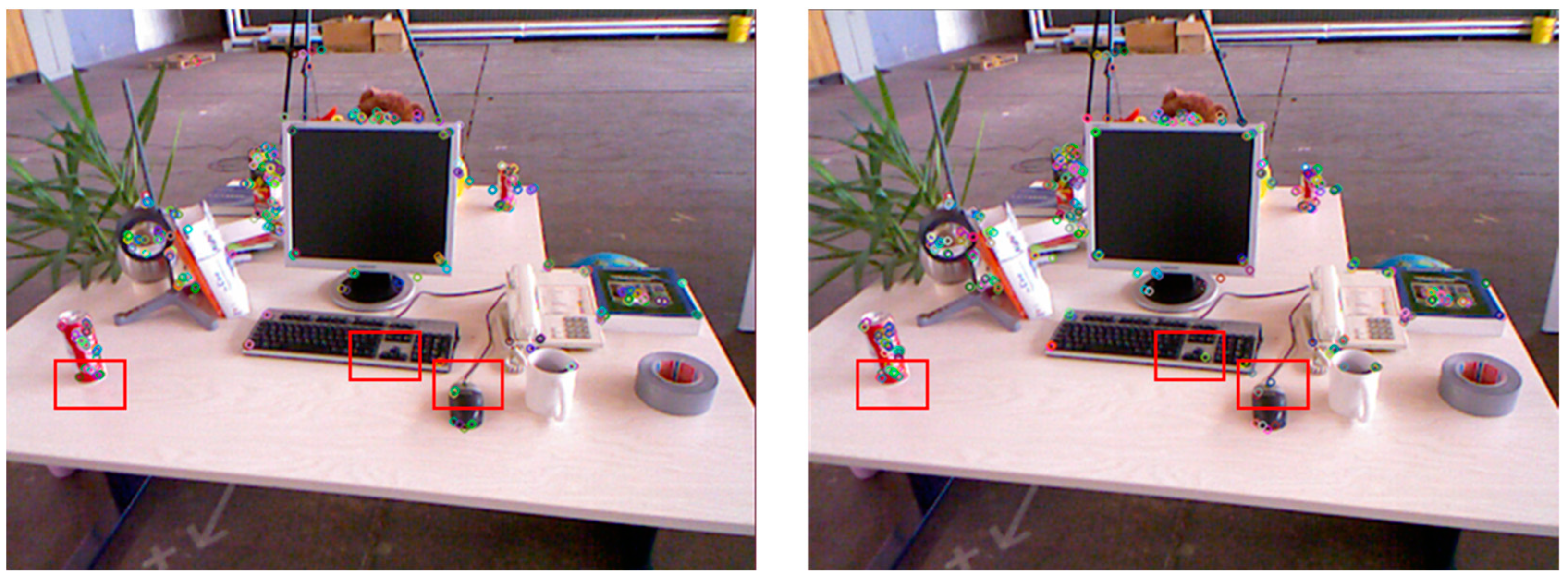
We first compared the feature extraction results for the same image by two feature extraction methods. As shown in Figure 5, we selected Figure 4a to perform the comparison experiment. Figure 5 shows that the improved AoFAST feature extraction algorithm can extract more feature points than the oFAST algorithm.
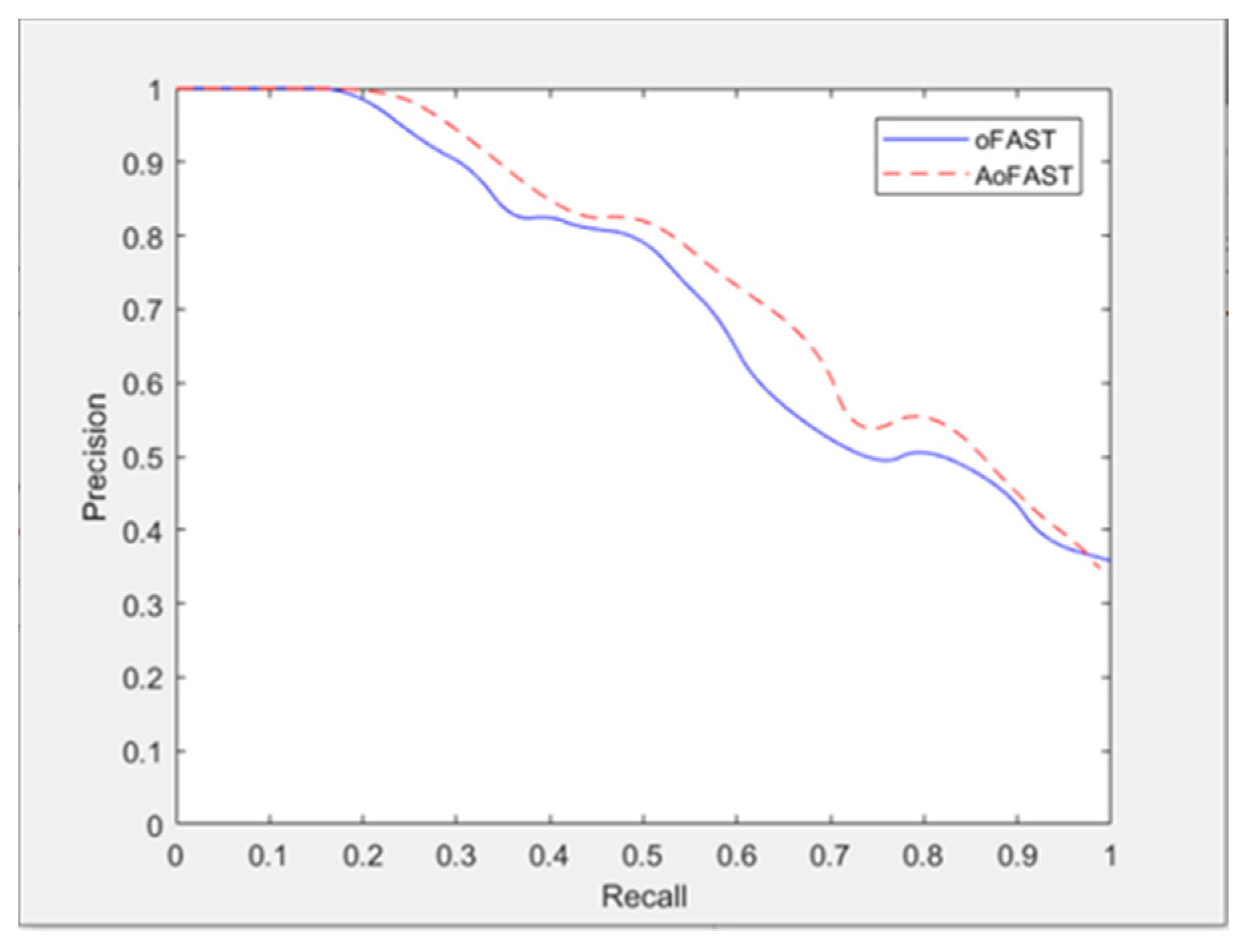
To prove that the points extracted from AoFAST are robust and were suitable for the following feature point matching, we conducted a feature point matching experiment based on two feature extraction methods. To compare the effects of the two methods, we used the precision–recall curve. The precision rate is and the recall rate is , which are calculated as Equations (16) and (17), respectively:
where is the true positive, which is the number of real matching points that are predicted as matching points; is the false positive, which is the number of real mismatching points that are predicted as matching points; and is the false negative, which is the number of real feature matching points that are predicted as mismatching points.
In the feature matching algorithm, high precision rate and high recall rate are simultaneously needed to obtain a larger number of correct correspondence points. However, this is challenging. The increase in recall rate is accompanied by a decline in precision rate. Therefore, a good algorithm has a higher precision rate under the same recall rate and higher precision rate under the effective recall rate.
Figure 6 compares the precision–recall of the oFAST and AoFAST algorithms. Obvious differences can be observed between the two curves. Under the same recall rate, the precision rate of AoFAST algorithm is better than that of the oFAST algorithm.
The above results show that the AoFAST feature extraction algorithm performs better in feature point extraction than oFAST. Calculation speed is also an important aspect of a feature extraction algorithm. Table 2 compares the time efficiency of oFAST and AoFAST. Table 2 shows that the calculation speed difference between the AoFAST and oFAST algorithms for the four pairs of images in Figure 4. Table 2 shows that the time difference between the two algorithms is less than 0.1 ms and both produced good real-time performance.
4.2.2. Experimental Results and Analysis of Image Feature Matching Algorithm
For PROSAC and RANSAC, we compared the ability of the two algorithms to eliminate the mismatching point pairs through an image matching experiment. Figure 7 shows that some obvious mismatches remain after RANSAC and PROSAC eliminates them. This proves that PROSAC’s ability to reject mismatching points is significantly better than RANSAC’s.
Similarly, we used the precision–recall curve to measure the performance of the two algorithms. Figure 8 depicts the result. We used the AoFAST feature extraction algorithm uniformly in the experiment. Figure 8 plots the precision rate and recall rate obtained by changing the thresholds of RANSAC and PROSAC.
From the precision–recall curve of RANSAC and PROSAC, when the recall rate is low, the precision rate of two algorithms are similar high because when the threshold is small, only few points are determined as interior points and these interior points have high precision. Since the threshold is small, many correct matching points remain that are not determined as interior points, so the recall rate is low. In practical applications, having too few feature points cannot meet the requirements of pose solution. When the recall rate gradually increases, especially when it is greater than 0.5, the precision rate of PROSAC is significantly higher than that of RANSAC, so can better satisfy the requirements of feature matching. This occurs because as the threshold increases, more interior points are selected into the interior point set and inevitably some exterior points are selected into the interior point set, so the precision rate of the interior point decreases while the recall rate increases. However, PROSAC has higher precision rate than RANSAC at the same recall rate, which is crucial for successfully solving camera poses. When the recall rate approaches 100%, all interior and exterior points are roughly selected into the interior point set and the accuracy of the two converges to a fixed value. The relationship between the recall rate and the precision rate shows that when the recall rate is too high, many exterior points are regarded as interior points and large uncertainty is introduced into the pose solution. When the recall rate is too low, there are few interior points, which cannot meet the requirements for a pose solution. A robust image matching method requires the best recall rate with enough correct interior points. Figure 8 shows that the PROSAC algorithm always has advantages over RANSAC algorithm in terms of precision rate under the same recall rate, especially when the recall rate is between 0.6 and 0.7. In this range, the number of interior points is sufficient and the precision rate is also high. This is consistent with the conclusion in the literature that the recommended recall value is around 0.65, which can ensure that the image matching interior point set can satisfy both the number and quality requirements [42].
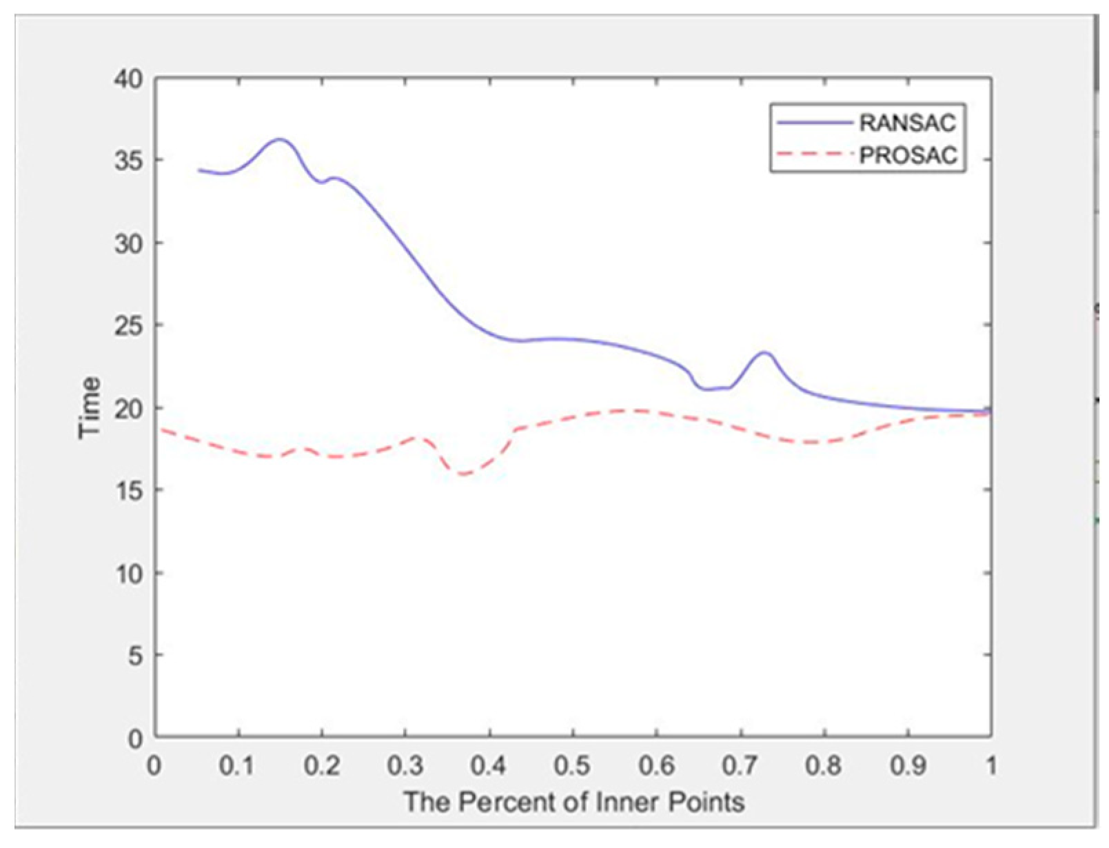
From the perspective of time cost, PROSAC is faster. Figure 9 shows the curve of time varying with the proportion of interior points when changing the threshold of RANSAC and PROSAC.
Figure 9 shows that the average time cost of PROSAC is significantly lower than RANSAC because the random sampling of the RANSAC algorithm leads to more iterations. In general, the average number of iterations is larger than one, so the time cost of the algorithm is relatively large. Since PROSAC pre-sorts the interior points, it can obtain better samples during the sampling process, so the number of iterations is far lower than the RANSAC algorithm. Generally, one iteration can obtain the correct model and the corresponding number of iterations is low. As the percentage of interior points increases, the probability that RANSAC selects the interior point when randomly selecting samples increases and the success rate of obtaining the correct model is correspondingly higher, so that the number of iterations decreases and the calculation time decreases. The running time of PROSAC is almost independent of the proportion of interior points and it is more robust to sample error. In general, when the proportion of interior points is less than 0.8, the time cost of PROSAC is significantly lower than that of RANSAC, which also increases the robustness of PROSAC to feature matching, especially for images with some mismatched points.
4.2.3. Experimental Results and Analysis of Different Epipolar Line Constraints
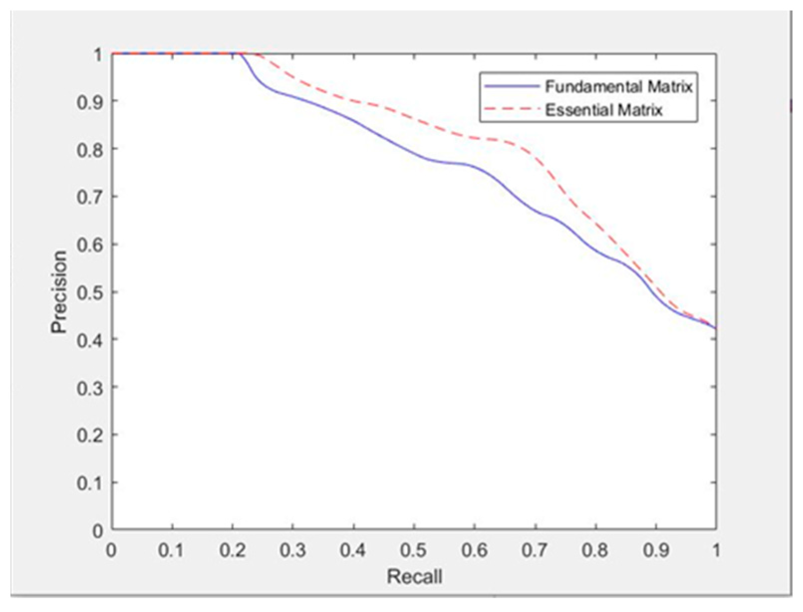
Figure 10 shows that the epipolar line constraint based on the essential matrix is better than that based on fundamental matrix because some mismatched pairs are better eliminated
Similarly, we used the precision–recall curve to compare the two algorithms. Figure 11 shows that curves of the two are different. Under the same recall rate, the precision rate of the matching results after the epipolar line constraint based on the essential matrix is significantly higher than that after the epipolar line constraint based on the fundamental matrix.
The four sets of data in Table 3 shows that the calculation speed of the epipolar line constraint based on the essential matrix is slightly faster than that based on the fundamental matrix.
4.2.4. Experimental Results and Analysis of Two Visual Odometry Methods
The aim of visual odometry is to restore the camera pose through image matching, which is achieved by solving the camera’s rotation matrix and translation vector. We compared the ORB-SLAM 2 visual odometry with the improved visual odometry through a pose recovery experiment using Figure 4c and calculated the translation vectors using two methods and compared them with the real value to determine accuracies of the two methods. The results are shown in Table 4.
The ground truth was measured using a TS60 measurement robot and the last two columns in Table 4 provide the results of the translation matrix solved by the two visual odometry methods. The visual odometry in this paper is more accurate than the original ORB-SLAM2 visual odometry method.
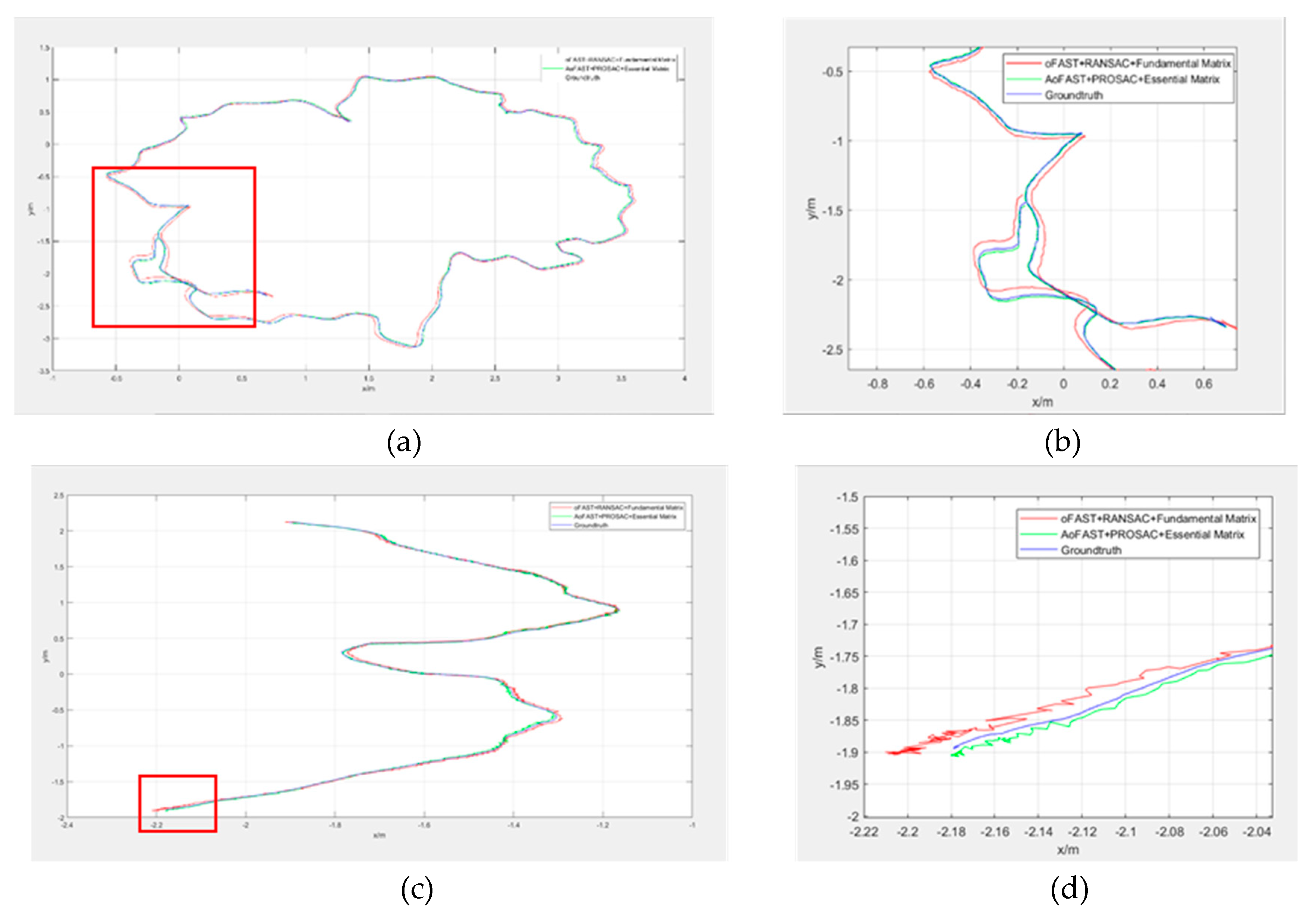
To further prove that the visual odometer method proposed in this paper provides excellent continuous camera pose calculation, we selected two video streams: the TUM data sets mentioned above, rgbd_dataset_freiburg2_desk (video 1) and rgbd_dataset_freiburg3_structure_texture_near (video 2), to conduct a continuous camera pose calculation experiment. First, the trajectories of the two methods were compared. As shown in Figure 12, the ORB-SLAM2 visual odometry and our method were used to estimate the pose for the same video stream and we compared the pose estimation. We all know that there is an incremental error in the camera pose calculation for each frame. With the accumulation of camera frames, the error is also accumulated accordingly, which makes the calculated camera trajectory more and more deviate from the real camera trajectory. This can be reflected obviously at the end of the trajectory. Therefore, the tails of the trajectories were selected separately for detailed observation and more intuitive and obvious differences were observed. Figure 12 shows that with the accumulation of cumulative error, our algorithm provides obvious advantages and its calculated trajectory is closer to the true trajectory of the camera, whereas the visual odometry of ORB-SLAM2 has a larger error.
Intuitive trajectory comparison shows that the visual cumulative error of the two visual odometry methods differs. The numerical difference between the cumulative errors of the two can be demonstrated from the perspective of data quantification. Table 5 shows the accumulated errors in X and Y directions when using ORB-SLAM2 visual odometry and our method to realize the pose estimation of the same video stream.
We used the ratio of the error to the total length to measure the effect of two methods, where the total length of the trajectory was provided in Section 4.1. Table 5 shows that in the Video1 experiment, the errors of the ORB-SLAM2 visual odometry method in the X and Y direction were 1.26% and 2.9% of the total length of the trajectory, respectively; the errors of our visual odometry method in the X and Y directions were 1.14% and 1.45% of the total track length, respectively, which is 9.62% and 50% less than ORB-SLAM2. In the Video2 experiment, the error rates in the X and Y directions of the ORB-SLAM2 visual odometry method were 1.41% and 1.13% of the total length of the trajectory, respectively; the error rates of our method in the X and Y directions were 0.9% and 0.7%, respectively, which are reductions of 34.5% and 41.91%, respectively.
We also compared the results of the two methods using the evaluation method provided by the TUM data set and obtained the results provided in Table 6. Table 6 provides the root mean square error (RMSE) and mean value of the translation error and rotation error of the two methods. For the four indicators of the two sets of data, our method produced better performance than ORB-SLAM2 visual odometry. Compared with the ORB-SLAM2 visual odometry method, the RMSE and mean value of the translation error of the two sets of data in this algorithm are reduced by 37.48%, 31.93%, 42.99% and 32.78%, respectively; the rotation error is reduced by 35.86%, 29.85%, 37.87% and 37.59%, respectively.
Time is also another key factor in visual SLAM. A good algorithm should be both accurate and fast. The same video stream data were implemented using the two methods and we compared their calculation speed. Table 7 lists the average time required for each pair of adjacent frame images, which is the time of the entire tracking thread divided by the number of image frames. The time cost of the proposed method is significantly less than that of the ORB-SLAM2 visual odometry method, which is reduced by 7.83% and 8.98% for Video1 and Video2, respectively.
5. Conclusions
Visual odometry is one of the key technologies in the field of visual SLAM, which has a wide range of applications in autonomous navigation, automatic driving and augmented reality. In this study, we addressed the problems experienced by ORB-SLAM2 visual odometry: robustness and cumulative error in the process of restoring camera pose. Based on the previous research, we created an improved visual odometry method. Specifically, this paper illustrated the following: (1) On the basis of ORB-SLAM2 visual odometry, the threshold value of feature extraction is obtained in an adaptive form and the AoFAST algorithm was proposed, which increases the robustness and stability of the feature extraction. (2) PROSAC is used instead of RANSAC to optimize the matching and improve the feature matching accuracy. (3) The epipolar line constraint based on the essential matrix is used to further refine the matching point pairs. (4) The performance of the proposed visual odometry and ORB-SLAM2 visual odometry were compared and analyzed using experiments. The experimental results showed that the proposed method is better than the ORB-SLAM2 visual odometry method in both accuracy and speed. The proposed method is efficient and precise in the calculation of camera motion trajectory, effectively optimizing the visual odometry estimation error and reducing the cumulative drift.
Author Contributions
Ming Li and Jiangying Qin proposed the methodology and wrote the paper; Jiangying Qin and Ming Li conceived and designed the experiments; Jiangying Qin, Ming Li, Xuan Liao and Jiageng Zhong performed the experiments.
Funding
This research was funded by the National Key R&D Program of China, grant numbers 2018YFB0505400 & 2016YFB0502202, the National Natural Science Foundation of China (NSFC), grant number 41901407, the Fundamental Research Funds for the Central universities, grant number 2042018kf0012.
Acknowledgments
The authors would like to thank the Technical University Of Munich (TUM) for the supporting data, and thank the LIESMARS of Wuhan university for the supporting computing environment. Meanwhile, we thank the editors and reviewers for their valuable comments.
Conflicts of Interest
The authors declare no conflict of interest.
References
- Mur-Artal, R.; Montiel, J.M.M.; Tardós, J.D. ORB-SLAM: A versatile and accurate monocular SLAM system. IEEE Trans. Robot. 2017, 31, 1147–1163. [Google Scholar] [CrossRef] [Green Version]
- Mur-Artal, R.; Tardós, J.D. ORB-SLAM2: An open-source SLAM system for monocular, stereo, and RGB-D cameras. IEEE Trans. Robot. 2017, 33, 1255–1262. [Google Scholar] [CrossRef] [Green Version]
- Yang, G.; Chen, Z.; Li, Y.; Su, Z. Rapid relocation method for mobile robot based on improved ORB-SLAM2 algorithm. Remote Sens. 2019, 11, 149. [Google Scholar] [CrossRef] [Green Version]
- Davison, A.J.; Reid, I.D.; Molton, N.D.; Stasse, O. MonoSLAM: Real-time single camera SLAM. IEEE Trans. Pattern Anal. Mach. Intell. 2007, 29, 1052. [Google Scholar] [CrossRef] [PubMed] [Green Version]
- Gupta, S.; Girshick, R.; Arbeláez, P.; Malik, J. Learning Rich Features from RGB-D Images for Object Detection and Segmentation. In Proceedings of the 13th European Conference on Computer Vision (ECCV 2014), Zurich, Switzerland, 6–12 September 2014; pp. 345–360. [Google Scholar]
- Huang, A.S.; Bachrach, A.; Henry, P.; Krainin, M.; Maturana, D.; Fox, D.; Roy, N. Visual Odometry and Mapping for Autonomous Flight Using an RGB-D Camera. In Proceedings of the 2017 15th International Symposium of Robotics Reasearch, Flagstaff, AZ, USA, 9–12 December 2011; pp. 235–252. [Google Scholar]
- Kerl, C.; Sturm, J.; Cremers, D. Dense visual SLAM for RGB-D cameras. In Proceedings of the 2013 IEEE/RSJ International Conference on Intelligent Robots and Systems, Tokyo, Japan, 3–7 November 2013; pp. 2100–2106. [Google Scholar]
- Lee, Y.J.; Song, J.B. Visual SLAM in Indoor Environments Using Autonomous Detection and Registration of Objects. In Proceedings of the IEEE International Conference on Multisensor Fusion and Integration for Intelligent Systems, Seoul, Korea, 20–22 August 2008; pp. 671–676. [Google Scholar]
- Wang, Y. Research on Binocular Visual Inertial Odometry with Multi-Position Information Fusion. Ph.D.’s Thesis, University of Chinese Academy of Sciences (Changchun Institute of Optics, Fine Mechanics and Physics, Chinese Academy of Sciences), Beijing, China, 2019. [Google Scholar]
- Muja, M.; Lowe, D.G. Fast Approximate Nearest Neighbors with Automatic Algorithm Configuration. In Proceedings of the Fourth International Conference on Computer Vision Theory and Application, Lisboa, Portugal, 5–8 February 2009; pp. 331–340. [Google Scholar]
- Chum, O.; Matas, J. Matching with PROSAC-Progressive Sample Consensus. In Proceedings of the 2005 IEEE Computer Society Conference on Computer Vision and Pattern Recognition, Washington, DC, USA, 20–26 June 2005; pp. 220–226. [Google Scholar]
- Brand, C.; Schuster, M.J.; Hirschmuller, H.; Suppa, M. Stereo-Vision Based Obstacle Mapping for Indoor/Outdoor SLAM. In Proceedings of the 2014 IEEE/RSJ International Conference on Intelligent Robots and Systems, Chicago, IL, USA, 14–18 September 2014; pp. 1846–1853. [Google Scholar]
- Yan, K.; Sukthankar, R. PCA-SIFT: A More Distinctive Representation for Local Image Descriptors. In Proceedings of the 2004 IEEE Computer Society Conference on Computer Vision and Pattern Recognition, Washington, DC, USA, 27 June–2 July 2004; pp. 506–513. [Google Scholar]
- Bay, H.; Tuytelaars, T.; Gool, L.V. SURF: Speeded Up Robust Features. In Proceedings of the 9th European Conference on Computer Vision, Graz, Austria, 7–13 May 2006; pp. 404–417. [Google Scholar]
- Leutenegger, S.; Chli, M.; Siegwart, R.Y. BRISK: Binary Robust Invariant Scalable Keypoints. In Proceedings of the IEEE International Conference on Computer Vision, Barcelona, Spain, 6–13 November 2011; pp. 2548–2555. [Google Scholar]
- Rublee, E.; Rabaud, V.; Konolige, K.; Bradski, G.R. ORB: An Efficient Alternative to SIFT or SURF. In Proceedings of the 2011 International Conference on Computer Vision, Barcelona, Spain, 6–13 November 2011; pp. 2564–2571. [Google Scholar]
- Hu, M.; Ren, M.; Yang, J. A fast and practical feature point matching algorithm. Comput. Eng. 2004, 30, 31–33. [Google Scholar]
- Mount, D.M.; Netanyahu, N.S.; Moigne, J.L. Efficient algorithms for robust feature matching. Pattern Recognit. 1997, 32, 17–38. [Google Scholar] [CrossRef] [Green Version]
- Fischler, M.; Bolles, R. Random sample consensus: A para-digm for model fitting with applications to image analysis and automated cartography. Commun. ACM. 1981, 24, 381–395. [Google Scholar] [CrossRef]
- Choi, S.; Kim, T.; Yu, W. Performance evaluation of RANSAC family. J. Comput. Vision 1997, 24, 271–300. [Google Scholar]
- Derpanis, K.G. Overview of the RANSAC Algorithm; Technical report for Computer Science; York University: North York, ON, Canada, May 2010. [Google Scholar]
- Schnabel, R.; Wahl, R.; Klein, R. Efficient RANSAC for Point-Cloud Shape Detection. Comp. Graph. Forum 2010, 26, 214–226. [Google Scholar] [CrossRef]
- Kitt, B.; Geiger, A.; Lategahn, H. Visual Odometry Based on Stereo Image Sequences with RANSAC-Based Outlier Rejection Scheme. In Proceedings of the 2010 IEEE Intelligent Vehicles Symposium, San Diego, CA, USA, 21–24 June 2010; pp. 486–492. [Google Scholar]
- Rusinkiewicz, S.; Levoy, M. Efficient Variants of the ICP Algorithm. In Proceedings of the Third International Conference on 3-D Digital Imaging and Modeling, Quebec City, QC, Canada, 28 May–1 June 2001; pp. 145–152. [Google Scholar]
- Gao, X.-S.; Hou, X.-R.; Tang, J.; Cheng, H.-F. Complete solution classification for the perspective-three-point problem. IEEE Trans. Pattern Anal. Mach. Intell. 2003, 25, 930–943. [Google Scholar]
- Zhu, Z.; Oskiper, T.; Samarasekera, S.; Kumar, R.; Sawhney, H.S. Ten-Fold Improvement in Visual Odometry Using Landmark Matching. In Proceedings of the 2007 IEEE 11th International Conference on Computer Vision, Rio de Janeiro, Brazil, 14–21 October 2007; pp. 1–8. [Google Scholar]
- Ramezani, M.; Acharya, D.; Gu, F.; Khoshelham, K. Indoor Positioning by Visual-Inertial Odometry. In Proceedings of the ISPRS Annals of Photogrammetry, Remote Sensing and Spatial Information Sciences, Wuhan, China, 18–22 September 2017; Volume 4, pp. 371–376. [Google Scholar]
- Acharya, D.; Ramezani, M.; Khoshelham KWinter, S. BIM-Tracker: A model-based visual tracking approach for indoor localisation using a 3D building model. ISPRS J. Photogramm. Remote Sens. 2019, 150, 157–171. [Google Scholar] [CrossRef]
- Gu, F.; Hu, X.; Ramezani, M.; Acharya, D.; Khoshelham, K.; Valaee, S.; Shang, J. Indoor localization improved by spatial context—A survey. ACM Comput. Surv. 2018, 52, 1–35. [Google Scholar] [CrossRef] [Green Version]
- Piasco, N.; Sidib, D.; Demonceaux, C.; Gouet-Brunet, V. A survey on visualbased localization: On the benefit of heterogeneous data. Pattern Recognit. 2018, 74, 90–109. [Google Scholar] [CrossRef] [Green Version]
- Venkatachalapathy, V. Visual Odometry Estimation Using Selective Features. Master’s Thesis, Rochester Institute of Technology, Rochester, NY, USA, July 2016; pp. 19–24. [Google Scholar]
- Huang, A.S.; Bachrach, A.; Henry, P.; Krainin, M.; Maturana, D.; Fox DRoy, N. Visual odometry and mapping for autonomous flight using an RGB-D camera. In Robotics Research; Springer: Cham, Southeast Asia, 2017; pp. 235–252. [Google Scholar]
- Xin, G.X.; Zhang, X.T.; Xi, W. A RGBD SLAM Algorithm Combining ORB with PROSAC for Indoor Mobile Robot. In Proceedings of the 2015 4th International Conference on Computer Science and Network Technology, Harbin, China, 19–20 December 2015; pp. 71–74. [Google Scholar]
- Chum, O.; Matas, J.; Kittler, J. Locally optimized RANSAC. Lecture Notes Comput. Sci. 2003, 2781, 236–243. [Google Scholar]
- Rosten, E.; Porter, R.; Drummond, T. Faster and better: A machine learning approach to corner detection. IEEE Trans. Pattern Anal. Mach. Intell. 2008, 32, 105–119. [Google Scholar] [CrossRef] [PubMed] [Green Version]
- Chum, O.; Werner, T.; Matas, J. Epipolar Geometry Estimation via RANSAC Benefits from the Oriented Epipolar Constraint. In Proceedings of the 17th International Conference on Pattern Recognition (ICPR 2004), Cambridge, UK, 26 August 2004; pp. 112–115. [Google Scholar]
- Kapur, J.N.; Sahoo, P.K.; Wong, A.K.C. A new method for gray-level picture thresholding using the entropy of the histogram. Comp. Vision Graph. Image Process. 1985, 29, 273–285. [Google Scholar] [CrossRef]
- Dubrofsky, E. Homography Estimation; Diplomová práce, Univerzita Britské Kolumbie: Vancouver, BC, Canada, 2009. [Google Scholar]
- Lepetit, V.; Moreno-Noguer, F.; Fua, P. Epnp: An accurate o(n) solution to the pnp problem. Int. J. Comput. Vision 2008, 81, 155–166. [Google Scholar] [CrossRef] [Green Version]
- Penate-Sanchez, A.; Andrade-Cetto, J.; Moreno-Noguer, F. Exhaustive linearization for robust camera pose and focal length estimation. IEEE Trans. Pattern Anal. Mach. Intell. 2013, 35, 2387–2400. [Google Scholar] [CrossRef] [PubMed] [Green Version]
- Hesch, J.A.; Roumeliotis, S.I. A Direct Least-Squares (DLS) method for PnP. In Proceedings of the IEEE International Conference on Computer Vision (ICCV 2011), Barcelona, Spain, 6–13 November 2011; pp. 383–390. [Google Scholar]
- Li, L. Research on indoor positioning algorithm based on PROSAC algorithm. Ph.D.’s Thesis, Harbin Institute of technology, Harbin, China, 2018. [Google Scholar]
Figure 1.
Flow chart of improved visual odometry.

Figure 2.
FAST feature extraction schematic.

Figure 3.
Polar geometry schematic.

Figure 4.
Four pairs of experimental images: (a) video stream data, (b) drone images, (c) mobile phone camera in Wuhan University Library and (d) mobile phone camera at the Wuhan University Remote Sensing Comprehensive Test Site.
Figure 4.
Four pairs of experimental images: (a) video stream data, (b) drone images, (c) mobile phone camera in Wuhan University Library and (d) mobile phone camera at the Wuhan University Remote Sensing Comprehensive Test Site.

Figure 5.
Comparison of feature extraction results between oFAST and AoFAST. Red rectangles are the highlight of the feature points that oFAST algorithm cannot extract while AoFAST can extract.
Figure 5.
Comparison of feature extraction results between oFAST and AoFAST. Red rectangles are the highlight of the feature points that oFAST algorithm cannot extract while AoFAST can extract.

Figure 6.
Comparison of precision–recall between oFAST and AoFAST.

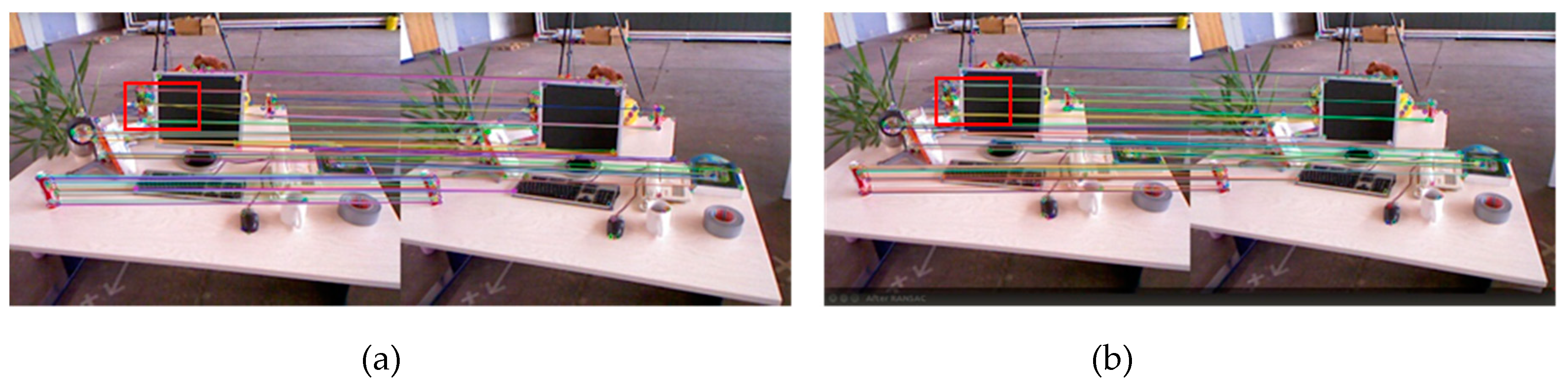
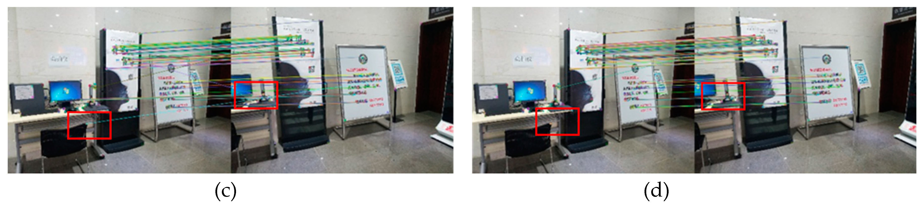
Figure 7.
Comparison of eliminating mismatches between random sample consensus (RANSAC) and PROSAC. (a,b) Results of the feature point extraction, (c) the result of the feature point matching without mismatching points elimination and (d,e) the results of culling the mismatching points after RANSAC and PROSAC. Red rectangles are the highlight of the mismatches that RANSAC cannot remove while PROSAC correctly removes.

Figure 8.
Comparison of precision–recall between RANSAC and PROSAC.

Figure 9.
Comparison of time proportion of interior points between RANSAC and PROSAC.

Figure 10.
Comparison of eliminating mismatches between two kinds of matrices: (a,c) the results of the epipolar line constraint using the fundamental matrix; (b,d) the results of the epipolar line constraint using the essential matrix. Red rectangles are the highlight of the mismatches that the epipolar line constraint using the fundamental matrix cannot remove while the epipolar line constraint using the essential matrix correctly removes.


Figure 11.
Comparison of precision–recall between two kinds of matrices.

Figure 12.
Comparison of trajectories between two methods of visual odometry. (a,c) The trajectory data of the two videos; (b,d) enlarged detail views of the boxed areas in (a,c), respectively.
Figure 12.
Comparison of trajectories between two methods of visual odometry. (a,c) The trajectory data of the two videos; (b,d) enlarged detail views of the boxed areas in (a,c), respectively.


Table 1.
Comparison of camera pose recovery methods.
| Method | Error (mm) | Time (ms) |
|---|---|---|
| PnP | 4.277 | 5.531 |
| EPnP | 1.311 | 5.111 |
| UPnP | 2.796 | 5.309 |
| DLS | 2.684 | 5.479 |
Table 2.
Comparison of time between oFAST and AoFAST.
| Image | oFAST (ms) | AoFAST (ms) |
|---|---|---|
| Figure 4a | 0.200 | 0.215 |
| Figure 4b | 0.401 | 0.447 |
| Figure 4c | 0.443 | 0.451 |
| Figure 4d | 0.429 | 0.444 |
Table 3.
Comparison of calculation speed between two kinds of matrices.
| Data | Fundamental Matrix (ms) | Essential Matrix (ms) |
|---|---|---|
| Figure 4a | 4.710 | 4.598 |
| Figure 4b | 5.351 | 5.346 |
| Figure 4c | 5.095 | 4.961 |
| Figure 4d | 5.826 | 5.809 |
Table 4.
Comparison of translation vectors between two methods of visual odometry.
| Direction | Ground Truth (M) | ORB-SLAM2 (m) | Our Method (m) |
|---|---|---|---|
| X | 0.905 | 0.909 | 0.904 |
| Y | –0.046 | –0.042 | –0.047 |
| Z | 0.421 | 0.414 | 0.424 |
| RMS | 0.009 | 0.003 |
Table 5.
Comparison of errors in X and Y directions between two visual odometry methods.
| Data/Direction | ORB-SLAM2 (cm) | Our Method (cm) |
|---|---|---|
| Video1 | ||
| X | 2.626 | 2.352 |
| Y | 4.868 | 2.410 |
| Video2 | ||
| X | –1.147 | 0.721 |
| Y | 1.365 | 0.793 |
Table 6.
Comparison of translation and rotation errors between two visual odometry methods.
| ORB-SLAM2 (m) | Our Method (m) | |
|---|---|---|
| Video1 | ||
| translational_error.rmse | 0.075 | 0.047 |
| translational_error.mean | 0.058 | 0.040 |
| rotational_error.rmse | 2.407 | 1.544 |
| rotational_error.mean | 1.969 | 1.382 |
| Video2 | ||
| translational_error.rmse | 0.047 | 0.027 |
| translational_error.mean | 0.034 | 0.023 |
| rotational_error.rmse | 1.002 | 0.964 |
| rotational_error.mean | 0.848 | 0.816 |
Table 7.
Comparison of time between two visual odometry methods.
| Data | ORB-SLAM2 (ms) | Our Method (ms) |
|---|---|---|
| Video1 | 28.613 | 26.373 |
| Video2 | 26.066 | 23.726 |
© 2019 by the authors. Licensee MDPI, Basel, Switzerland. This article is an open access article distributed under the terms and conditions of the Creative Commons Attribution (CC BY) license (http://creativecommons.org/licenses/by/4.0/).
Share and Cite
MDPI and ACS Style
Qin, J.; Li, M.; Liao, X.; Zhong, J. Accumulative Errors Optimization for Visual Odometry of ORB-SLAM2 Based on RGB-D Cameras. ISPRS Int. J. Geo-Inf. 2019, 8, 581. https://0-doi-org.brum.beds.ac.uk/10.3390/ijgi8120581
AMA Style
Qin J, Li M, Liao X, Zhong J. Accumulative Errors Optimization for Visual Odometry of ORB-SLAM2 Based on RGB-D Cameras. ISPRS International Journal of Geo-Information. 2019; 8(12):581. https://0-doi-org.brum.beds.ac.uk/10.3390/ijgi8120581
Chicago/Turabian StyleQin, Jiangying, Ming Li, Xuan Liao, and Jiageng Zhong. 2019. "Accumulative Errors Optimization for Visual Odometry of ORB-SLAM2 Based on RGB-D Cameras" ISPRS International Journal of Geo-Information 8, no. 12: 581. https://0-doi-org.brum.beds.ac.uk/10.3390/ijgi8120581
Note that from the first issue of 2016, this journal uses article numbers instead of page numbers. See further details here.