Application of AHP to Road Selection

1
Faculty of Geomatics, Lanzhou Jiaotong University, Lanzhou 730070, China
2
National-Local Joint Engineering Research Center of Technologies and Applications for National Geographic State Monitoring, Lanzhou 730070, China
3
Gansu Provincial Engineering Laboratory for National Geographic State Monitoring, Lanzhou 730070, China
4
Key Laboratory of Urban Land Resources Monitoring and Simulation, Ministry of Land and Resources, Shenzhen 518000, China
*
Author to whom correspondence should be addressed.
ISPRS Int. J. Geo-Inf. 2020, 9(2), 86; https://0-doi-org.brum.beds.ac.uk/10.3390/ijgi9020086
Submission received: 12 October 2019
/
Revised: 13 January 2020
/
Accepted: 27 January 2020
/
Published: 1 February 2020
(This article belongs to the Special Issue Map Generalization)
Abstract
:The analytic hierarchy process (AHP), a decision-making method, allows the relative prioritization and assessment of alternatives under multiple criteria contexts. This method is also well suited for road selection. The method for road selection based on AHP involves four steps: (i) Points of Interest (POIs), the point-like representations of the facilities and habitations in maps, are used to describe and build the contextual characteristic indicator of roads; (ii) form an AHP model of roads with topological, geometrical, and contextual characteristic indicators to calculate their importance; (iii) select roads based on their importance and the adaptive thresholds of their constituent density partitions; and (iv) maintain the global connectivity of the selected network. The generalized result at a scale of 1:200,000 by AHP-based methods better preserved the structure of the original road network compared with other methods. Our method also gives preference to roads with relatively significant contextual characteristics without interfering with the structure of the road network. Furthermore, the result of our method largely agrees with that of the manual method.
1. Introduction
The automatic generalization of geographic information is still a challenge in the field of cartography. Road selection is one of the main operations in topographic map generalization. It aims to maintain global and local patterns [1,2] and connectivity [3,4,5] of the original road network while reducing the level of detail in the road network. According to the representation mode of road networks, road selection methods can be broadly categorized into mesh-based methods, line-based methods, and combined line-mesh methods [6].
Mesh-based methods indirectly select roads by aggregating the meshes enclosed by road segments in terms of certain constraints (for example, the mesh area is less than the pre-defined threshold) [7,8,9,10,11]. The density pattern and connectivity of the road network can be better retained through these methods [10]. However, this method is not applicable to networks that are unable to construct areas and seldom takes into account the topological characteristics of roads.
Line-based methods are the most commonly used methods in road selection. They are realized by directly deleting roads in a ranked order [1,2,3,4,12,13,14,15,16,17,18,19,20,21,22,23,24]. In this group of methods, much attention is paid to topological relationships. For example, guided by graph theory, road networks are manipulated as connected graphs to perform road selection. Some conceptions like shortest path [12], minimum-spanning-tree [3], and centrality [4] are included to guide road selection. However, the centrality approach is unable to maintain the density distribution of original road networks and neglects some factors in actual road networks, such as roundabouts, dead ends, etc. Weiss and Weibel [13] developed some extensions in response to the aforementioned problems, realizing desirable selection results at small scales.
Line-mesh combination methods achieve selection by successively aggregating meshes and selecting the line features attached to those meshes. These combination methods focus on the individual meshes or lines in road networks, thus performing better than separate methods at medium scales [6,25]. However, different results might be produced by using different combination strategies of lines and meshes. Hence, this method needs to be further explored [26].
Compared with other map features, roads, as a linear feature, have noticeable characteristics in their connectivity and continuity. Fractured and disconnected networks can easily be generated by selection based on road segments. To avert this drawback, Thomson and Richardson proposed the concept of “strokes” based on the good continuation principle of perceptual grouping [15]. In this method, several neighboring road segments are grouped into a stroke, which is then treated as a unit in the selection process. This concatenation mode is widely used in line-based methods and line-mesh methods due to its superiority in maintaining the longitudinal hierarchy and geometric features of the original network. In addition, with the development of volunteered geographic information (VGI), methods that employ big data have come into being, thus widening the clues and perspectives of road selection studies. Points of Interest (POIs)have been adapted in recent years to regulate road selection. Xu et al. developed parameters such as POI density and the ratio of significant POIs around a road to reflect the contextual characteristics of roads [22]. However, this method is insufficient to distinguish the relative importance of different categories of POIs. For transportation purposes, Yu et al. added constraints between strokes by using taxi trajectory data [27]. Benz proposed the concept of POI accessibility. He argued that the paths to POIs should be retained in the selection process to enhance the practicality of the generalized results [25]. In addition, some objective weighting methods, such as Criteria Importance Though Intercriteria Correlation (CRITIC) [17,26,28], entropy [24], and coefficient of variation [22], were introduced to regulate the influence of different indicators on road selection. These methods have a strong mathematical basis, and are able to avoid different selection results caused by differences in cartographic experience. However, the determined weights often fail to reflect the actual importance of the indicators in the road selection environment. For instance, betweenness centrality should be given a higher weight in small-scale generalization due to its ability to identify the main hubs in a network [13]. While a road’s frequency of usage, type, width, length, and degree centrality also play a vital role in generalization at medium scales, these indicators contain local information about roads and reflect the relations between roads and their neighboring facilities. Hence, these methods lead to the weights of indicators being inconsistent with cartographic experience. In this regard, the analytic hierarchy process (AHP) [29], a multiple criteria decision-making tool, was introduced into road selection.
In the AHP model, superior alternatives can be identified. AHP has been applied to almost all fields involving decision-making, since its invention [30]. Rather than pursuing complex mathematical methods, AHP employs pairwise matrices and their associated right-eigenvectors to generate appropriate priority sequences of alternatives [29]. AHP is tolerant of different math tools, like linear programming, fuzzy logic, etc., whose merits can thus be extracted to achieve a desired outcome. Further, AHP organically combines qualitative and quantitative methods and decomposes a decision into a multi-level hierarchical structure. In this way, decision makers’ thinking processes are systematized and simplified. Both cartographic experience and the relations between indicator values can be incorporated into the evaluation system.
This is the first application of AHP in road selection. As a line-based method, our method is suitable for small-scale generalization. In addition, the surrounding habitations and facilities of a road can influence the importance of roads. In this regard, apart from summarizing structural characteristic indicators, an indicator reflecting the contextual characteristics of roads is built by scoring different categories of POIs. The importance values of strokes can be calculated in the AHP model, and the result of AHP serves as the fundamental basis for road selection. This method fully captures the attribute information of roads and conducts the road evaluation process in a structured and organized manner, which can be easily accepted. AHP delves deeper into the nature of road evaluation, multiple indicators, and the internal relations of roads.
The remainder of this paper is organized as follows. Section 2 begins with an introduction to AHP. In Section 3, a road evaluation strategy based on AHP is proposed. Section 4 offers a density maintenance solution based on adaptive thresholds. Section 5 elaborates the detailed selection process as well as a connectivity maintenance algorithm. In Section 6, attention is turned to validations of the proposed approach. Finally, some conclusions are made in Section 7.
2. Basic Theory of AHP
AHP offers the concept of hierarchy when handling problems related to a number of criteria and alternatives. In this model, factors involved in the corresponding level are compared in a pairwise manner, and a numeric scale is designed to calibrate the subsequent results. AHP usually employs the following subsections.
2.1. Structuring the Target Problem in a Hierarchy
Broaden the problem into a hierarchical structure composed of following levels: a goal, criteria, sub-criteria and alternatives. In the AHP model, the goal of the problem forms the top level. The intermediate levels constitute the criteria and sub-criteria. The bottom level comprises the decision-making alternatives.
2.2. Computing the Weight Vector of the Criteria
Suppose a total of criteria participate in pairwise comparison. An matrix is constructed. Each entry in matrix represents the relative importance of the th criterion with respect to the th criterion, which is characterized by: ① ; ② ③ . is determined numerically according to the ratio-scale ranging from 1 to 9. It covers the entire comparison spectrum, as shown in Table 1. Finally, perform a calculation to find the maximum eigenvalue and its corresponding eigenvector of matrix :
where represents the priority weight of the th criterion.
Then, calculate the consistency index and the consistency ratio using Formulaes (2) and (3) to verify the effectiveness of the comparison matrix .
where is the order of matrix , is mean random consistency index and can be determined by Table 2. If < 0.1, the comparison matrix conforms to the consistency standard.
2.3. Computing the Score Matrix of Alternatives
Given alternatives altogether, compare each alternative, whose results are calibrated on the numerical scale in Table 1 to develop an matrix with respect to the th criterion,. Each entry in matrix stands for the relative importance of the th alternative compared with the th alternatives under the th criterion. Find the maximum eigenvalue and its corresponding eigenvector of matrix . Finally, the weight vectors are grouped into the score matrix :
2.4. Computing the Global Alternative Scores
The global scores are finally obtained by multiplying the score matrix S and the weight vector .
The priority of the th alternative depends on the entry of .
3. Road Importance Evaluation Strategy Based on AHP
3.1. Road Network Maps
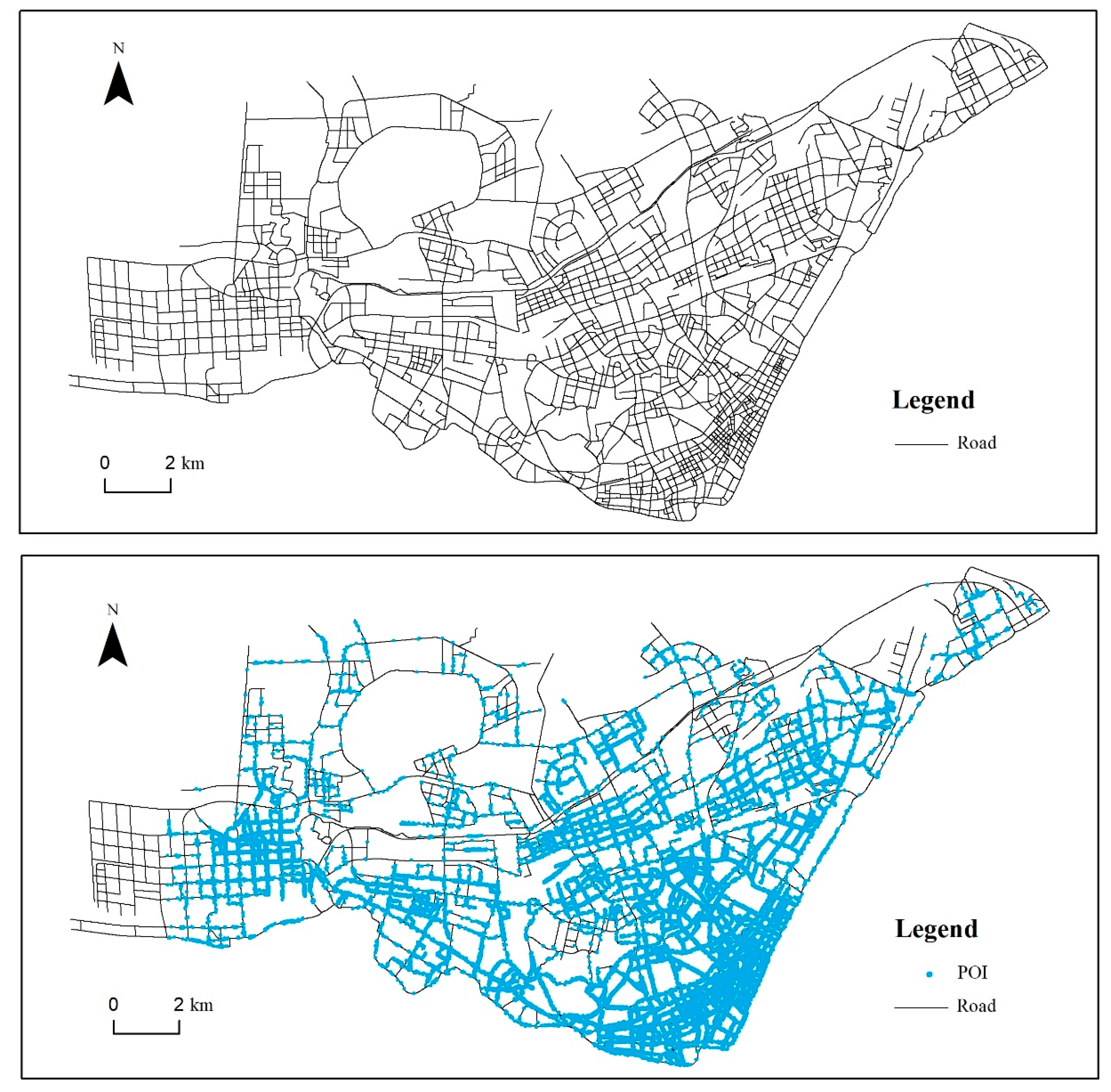
As shown in Figure 1, the experimental dataset was collected from the road network from Hankou District, Wuhan City, China, at a scale of 1:5000 and contains a total of 2815 segments. A total of 65,650 POIs inside road buffers were fetched from the open platform of Amap (http://lbs.amap.com/) by a Python crawler. Amap is a Chinese supplier of digital map content, navigation, and location services solutions., so the aforementioned website is in Chinese.
The roads in the map present a discernable distribution pattern. The roads in the lower-right corner are more densely distributed and surrounded by more POIs. These roads constitute the commercial center of the district. The roads and POIs in the upper areas are relatively sparse and represent the sub-urban areas.
3.2. Linegraph and Structural Characteristic Indicators of the Road Network
In road selection studies, when using graph theoretic principles, there are two kinds of common representations of road networks: one is to present roads as edges and road intersections as nodes, and the other is to map a road network onto a line graph, with roads as nodes and road intersections as edges.
The line graph can be defined by a simple unweighted graph , where and are the number of nodes and connected edges, respectively. The advantage of a line graph is that it is able to depict the connecting relationships between roads, the status of roads in a network, and the local and global efficiency of road networks clearly [31]. Hence, a line graph aids in the in-depth analysis of the structural characteristics and overall morphology of a road network [32].
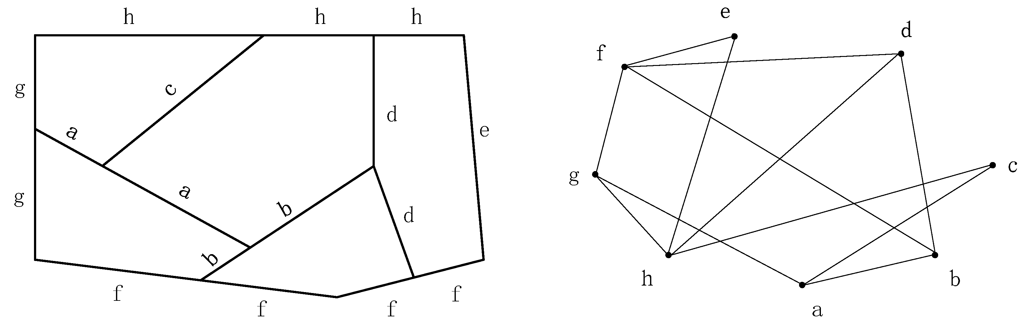
The practice of treating strokes, sets of road segments, as the selection unit has been widely accepted in previous research. Strokes are usually generated in terms of the semantic consistency or deflection angle threshold between neighboring road segments. Some studies have argued that a deflection angle threshold within a range of 40°~60° is optimal [33]. However, Weiss and Weibel [13] used a series of hierarchical angle thresholds according to road classes. This solution generated more reasonable stroke networks. Due to the lack of road class information, we adapted the standard method of setting the deflection angle to 45° to generate strokes.
Figure 2 shows an example to illustrate the methods mentioned above. To the left is a stroke network generated based on a deflection angle of 45°, while to the right is the corresponding line graph.
Geometrical characteristics and topological relations are the most fundamental and important attributes of roads and the key factors that affect the function of road networks. The relevant information for these attributes is inherent in road networks. Thus, they are highly practical to reflect the importance of roads [19]. Derived from a line graph, centrality indicators are used to measure the topological characteristics of roads, which can be mathematically summarized as degree centrality, betweenness centrality, and closeness centrality [4]. As a global indicator, betweenness centrality measures to what extent a road lies in between the paths connecting other roads and has the advantage of revealing the hierarchical importance of roads [13]. In this algorithm, the shortest distances from a given node to all other nodes within a network need to be calculated. So betweenness centrality is computationally expensive in practice. Although ,, and measure the importance of a stroke from a local perspective, they potentially identify the status of a stroke from the aspect of a structure. Closeness centrality measures to what extent a road is close to the center of a network, without representing the structural characteristics of roads. Thus, betweenness centrality and degree centrality are included in our approach. Since it is not guaranteed that a road with significant topological properties will function well in the network, the length of the stroke is introduced to measure the geometric characteristics of roads.
3.3. Contextual Characteristic Indicator of Roads
In addition to the structural characteristics of roads, it is also necessary to consider the surrounding habitations and facilities. Roads surrounded by key facilities tend to be more significant. Conversely, if the habitations and facilities around a road are sparse and insignificant, its status in the network might be lowered. For example, Wangfujing street in Beijing is not prominent in terms of structural characteristics. However, as a well-known commercial street in Beijing, it enjoys high recognition among people and performs a very important function. Furthermore, map features are constrained by their spatial interactions. The generalization of road networks should not be isolated from other features. Specifically, roads and their neighboring habitations are associated cartographic elements on maps [34,35]. This addition embodies the theory of the cooperative generalization of multiple features. In this regard, consideration should be given to the content of surrounding habitations and facilities to enhance the practicability and scientific rigor of road evaluation. To accomplish this, an indicator is built to define the contextual characteristics of roads assisted by POIs.
3.3.1. POI
A POI is a general term for any geographic entities that can be expressed using points, especially facilities and habitations. POI data are highly integrated and up to date. As point-like representations of habitations, POIs contain abundant relevant information, which can be used to assist in measuring the effects of contextual facilities on roads. According to existing studies and standard specifications [22,34], POIs within a buffer of 30 m from roads are regarded as habitations and facilities that are able to exert an influence on roads. In addition, due to the different sources of POI datasets, there are diverse POI classification criteria. Our objective is to distinguish differences in the importance of POIs by their classification. From this point of view, an official and unified classification of POIs is required. In this way, POIs are reclassified in line with the national standards for urban land classification (the code for the classification of urban land use and planning standards of development land GB50137-2011). The classification details are listed in Table 3.
3.3.2. Building the Contextual Characteristic Indicator
Different categories of POIs have unequal influence on the status of a road. Thus, when measuring the contextual characteristics of strokes, the Delphi method [36] is introduced to score POIs in terms of their categories, thereby differentiating and quantizing the influence of different POIs.
The Delphi method is a widely accepted method used to gather insights from respondents. It aims to discover a complete range of options, potential assumptions and associated judgements and eventually reaches a consensus on a real-world topic. This method conducts a series of questionnaires repeatedly to collect feedback from the respondent group.
When receiving the questionnaires, the experts are required to make judgments of “not significant”, “not very significant”, “generally significant”, “rather significant” or “quite significant” for each category of POIs. According to a 5-point Likert scale, the above five types of judgments are assigned scores of 1 to 5. The attributes of some categories of POIs can be measured with industrial or national standards or via common sense. For example, the shopping service category can be clearly classified into supermarkets, general shopping malls, and small shops according to business scopes. Tourist attractions can be classified into world heritage sites, national attractions, provincial attractions, and other attractions. Medical care can be divided into general hospitals, specialized hospitals, clinics, and pharmacies. Therefore, when making judgments, on the one hand, experts should consider the influence of POIs on the importance of roads. On the other hand, they should distinguish the differences of the attributes and characteristics within one category. Assume that among eight cartographers, the numbers of experts scoring 1 to 5 for the th category of POIs are , , , and , respectively, and the final score of the th category is calculated as:
Scores for partial POI categories are shown in Table 4.
Both the number and importance of different categories of POIs alongside a stroke are indispensable parameters to determine the influence of contextual habitations and facilities. Gather the statistics for the number and categories of POIs inside the buffer of the th stroke, and the contextual characteristic indicator can be calculated by the following formula:
where is the number of the POIs of the th category inside the buffer of the th stroke, and is the score of the th category. Unlike betweenness centrality, the measures the local characteristics of a road, so the indicator takes less computation time.
3.4. Stroke Importance Evaluation Based on AHP
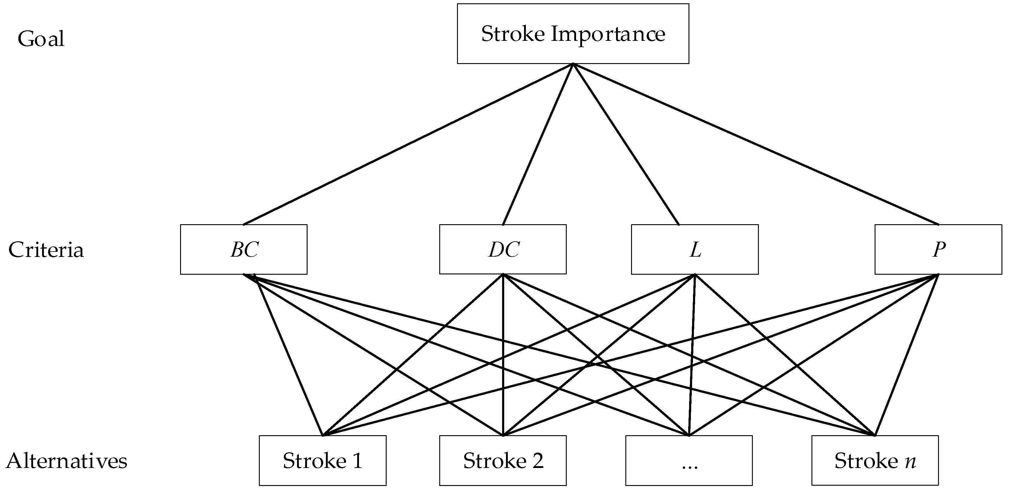
In the model of AHP, the elements in the corresponding level are compared in a natural, pairwise manner, and their results are then synthesized to assist decision makers. Not only does this systematic and structured method make full use of attribute information, but it is also in line with human cognition [35]. In this paper, AHP is introduced to compute the priority weights of stokes. The betweenness centrality, degree centrality, contextual characteristic indicator, length (corresponding to , , , and , respectively) are integrated in the procedure to measure strokes from the perspective of their geometrical, topological, and contextual characteristics. The AHP model based on stroke importance is shown in Figure 3.
The proposed method is divided into the steps listed below:
Step 1: The values of the , , , and of each stroke are calculated first. These four indicators are regarded as the criteria in AHP. Assume that there are strokes in the networks, then a matrix of 4 can be constructed:
Step 2: Calculate the weights of the indicators
The weights of the indicators are determined by evaluating their effects on the importance of the strokes. measures the importance of strokes in terms of the global and structural aspects of a network, so has a more significant effect on strokes. , and contain the local information of a stroke, so they are less important compared to . According to the ratio-scale in AHP (Table 2), the comparison matrix of the four indicators is shown in Table 5. The consistency ratio indicates that comparison matrix is completely consistent.
Then, calculate the corresponding eigenvector of matrix to obtain the weight vector of the indicators: [0.4, 0.2, 0.2, 0.2].
Step 3: Calculate the score matrix of the strokes
Given total strokes in a network, construct an pairwise comparison matrix , 1, 2, 3, 4 with respect to the indicators ,, and , respectively, whose entry indicates the relative importance of the th stroke compared to the th stroke under the th criterion. Note that if the th indicator value of the th or the th stroke is 0, then . Then, find the maximum eigenvalue and its eigenvector of matrix according to Section 2. The weight vectors are grouped into the score matrix .
Step 4: Multiply score matrix and the indicator weight vector to obtain the final scores of the strokes.
4. Adaptive Thresholds Based on Road Density Partition
Since the density distribution of roads on maps is heterogeneous, the selection results should reflect the contrast in the road density of different regions, to avoid the flattening or reversal of the density of a road network [37,38]. In our method, the stroke importance in urban areas tends to be relatively high. Because the values of and of the strokes in cities are higher, more roads in denser areas should be eliminated, while fewer roads should be eliminated in less dense areas in the generalization process. Considering the work of Tian [37] and Weiss and Weibel [13], we included a road density partition method based on Voronoi diagrams. The adaptive thresholds for stroke importance are pre-determined to regulate the selection process.
4.1. Road Density Partition
The basic idea of this method is that road intersections and endpoints are densely distributed in dense regions of the road network, while there are opposite situations in sparse regions. First, Voronoi diagrams of road intersections and endpoints are constructed to partition the entire map. The dense regions of the road network correspond to the clusters of Voronoi units of a small area. Similarly, the sparse regions correspond to the clusters of Voronoi units of a large area. Then, Getis-Ord Gi*, a hot spot analysis tool, is used to extract statistically high-value clustered regions and low-value clustered regions based on the area of the Voronoi units. Finally, the centroid points of the strokes are extracted. Their locations are then used to determine the density regions that the strokes belong to.
4.2. Preset Adaptive Thresholds Based on Road Density Partition
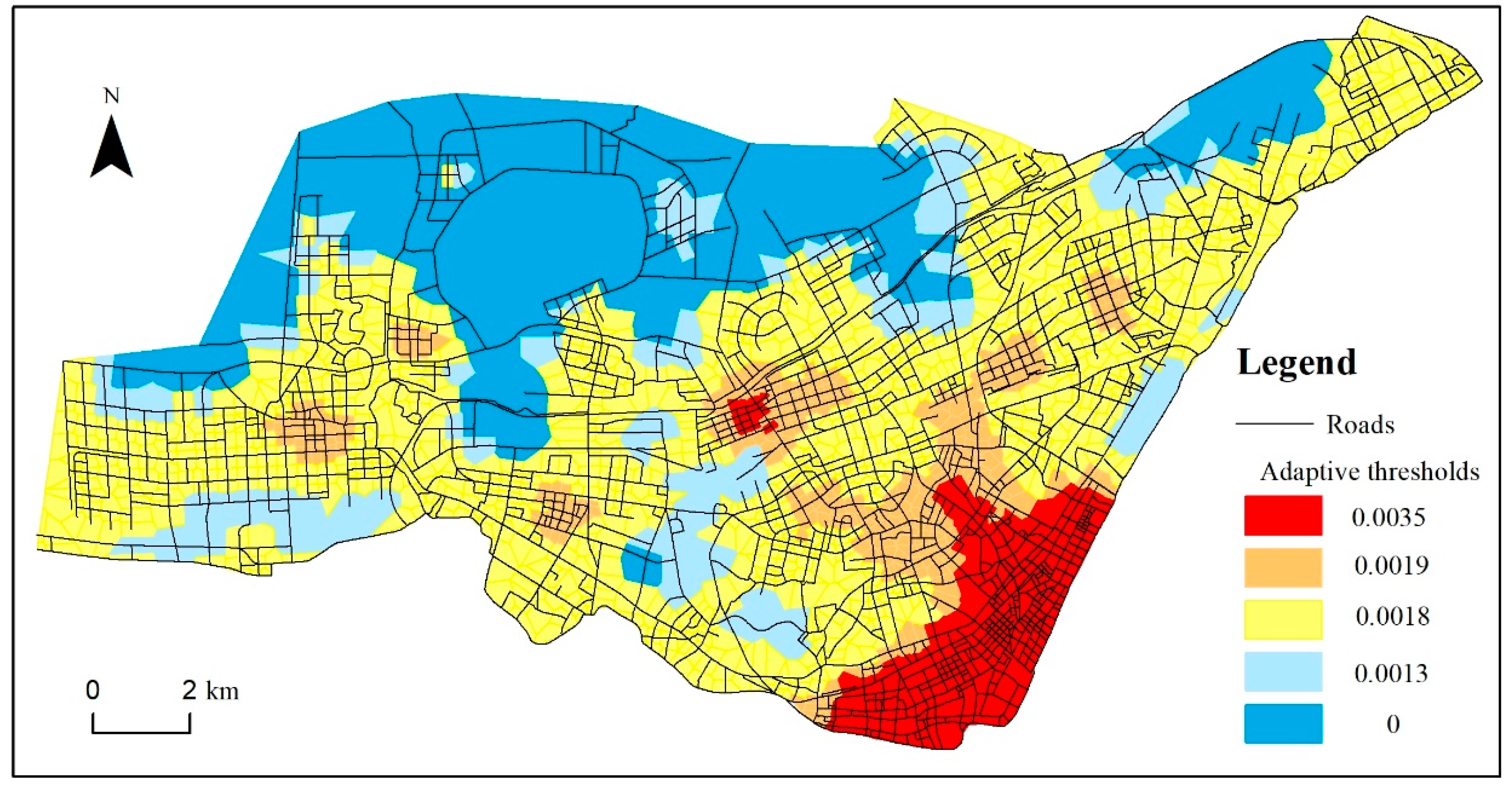
After the determination of the density regions of individual strokes, the adaptive thresholds for stroke importance are assigned to these clustered regions according to the importance values of their corresponding strokes. The principle for setting thresholds is to ensure the reservation of significant roads in each region and to exclude as many insignificant strokes as possible. Denser areas are constrained by more stringent thresholds. A stroke with a lower importance than the threshold is winnowed out when making selective omission decisions. The results of the road density partition and the preset thresholds for our test area are shown in Figure 4.
5. Road Selection Process
5.1. Overall Idea
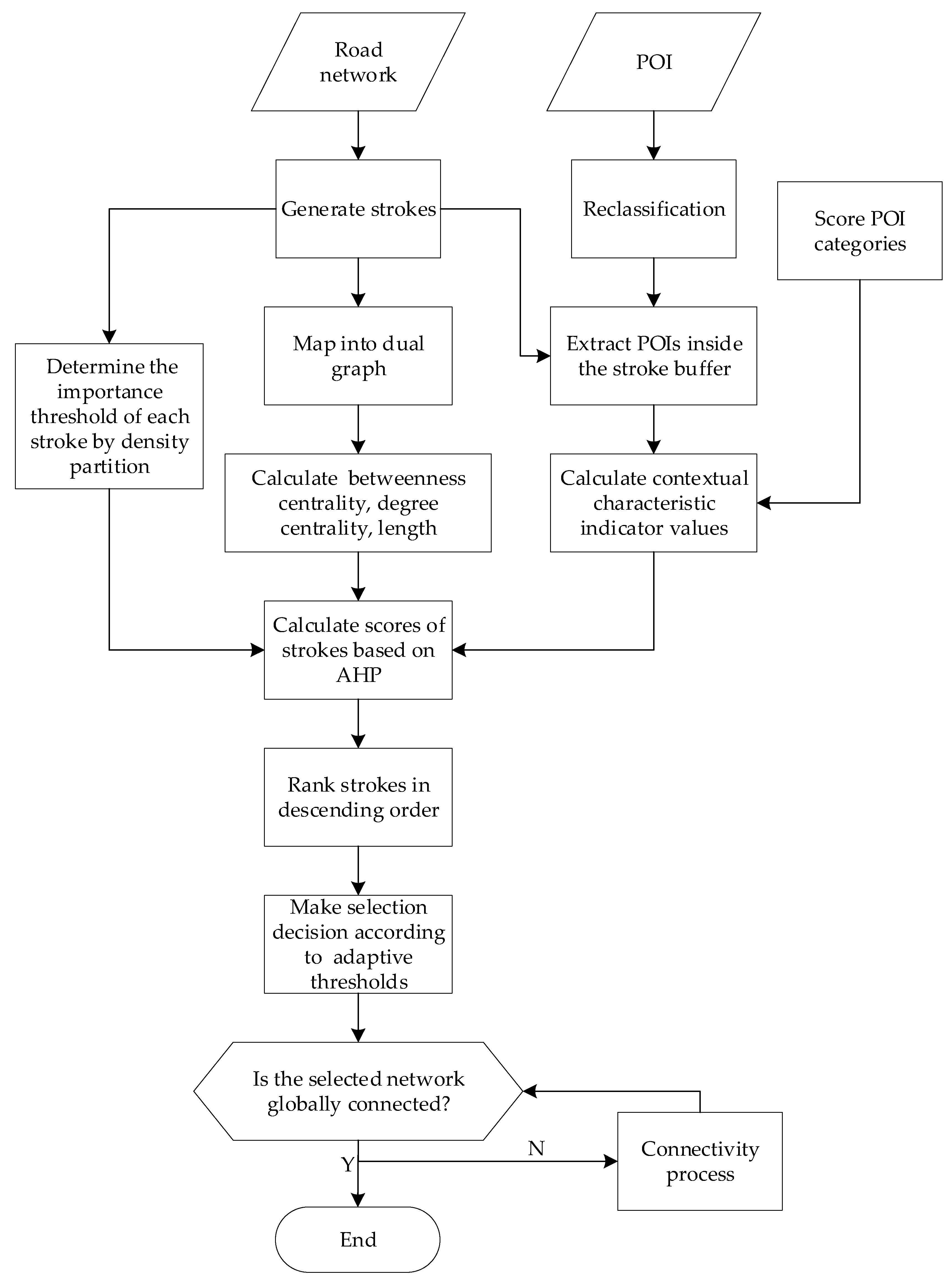
In the proposed method, four indicators are considered in the selection process, ,, and . The values of these indicators are aggregated into AHP to calculate the scores of strokes, which are then used to rank the strokes. This procedure is done in four main steps:
- (1)
- Extract the indicator values of the strokes: Generate the stroke network by setting the deflection angle as 45° and obtain the length of strokes. Calculate the contextual characteristic information assisted by the POIs inside the stroke buffer. Map the stroke network into a line graph to calculate the centrality indicator values.
- (2)
- Conduct a density partition using a Voronoi diagram and Getis-Ord Gi* to determine the importance threshold of each stroke.
- (3)
- Compute the scores of the strokes by the AHP-based method in Section 3.4, and select strokes in the descending order of the calculated scores. If the score of a stroke is higher than its corresponding importance threshold, the stroke is selected. This selection process continues until the total number is higher than the result calculated by the radical law method.
- (4)
- If the selected road network is disconnected, then the connectivity maintenance process in Section 5.2 is performed to keep the road network globally connected. Figure 5 shows the specific process of the proposed method.
5.2. Connectivity Maintenance
The generated stroke networks that are selected according to the importance ranking might break up into several disconnected parts, which is unacceptable. Some insignificant strokes connecting these disconnected parts should also be retained. Hence, a connectivity maintenance algorithm is proposed to be used in the selected network. We argue that the following principles should be followed when maintaining connectivity: add as few new strokes as possible and give priority to strokes of higher importance. In this regard, we define the weights of edges in the line graph of a stroke network and generate a spanning tree with the edges of maximum weight to maintain global connectivity.
5.2.1. Define Edge Weights for Line Graph
Edges in an unweighted complex network feature different significance [39]. To calculate the weights of these edges, we consider the importance of their constituent nodes. The edge weight of the two connecting nodes and is defined as:
where and are the scores of the corresponding strokes of nodes and , respectively. In this way, the line graph of the stroke network is converted into a weighted graph.
5.2.2. Connectivity Maintenance Algorithm
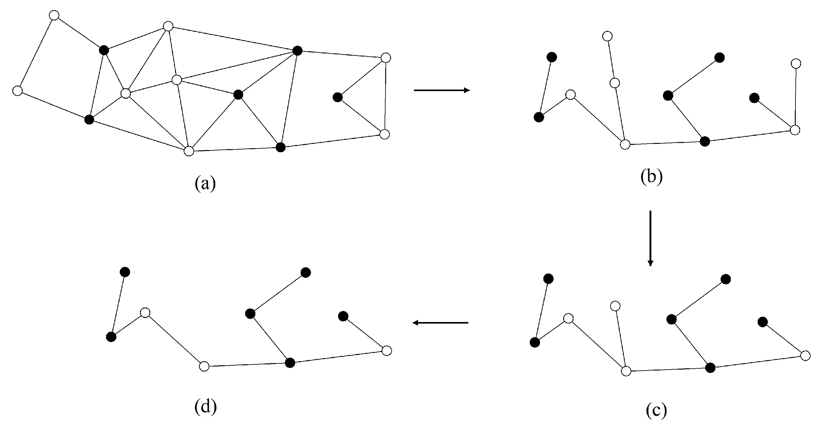
Figure 6a, for example, represents a line graph of the original road network. The black node set represents the selected strokes according the score ranking, while the white nodes represent the rest of the strokes in the original network. One can see that the generated graph is disconnected. The steps to maintain connectivity are as follows:
(1) Calculate the weights of edges in the original line graph by the formula in Section 5.2.1.
(2) Build a new spanning tree , in which , = 0. Each node in is regarded as a separate tree.
(3) Add the edges selected from in descending order of weight to . The nodes constituting the selected edges ought to belong to different trees, which are then merged into one tree, after selecting the edges.
(4) Repeat step (3) until all nodes are included in one tree, as shown in Figure 6b.
(5) Iteratively determine whether a leaf node in belongs to the selected node set ; if not, then delete it. This step ends until there are no white leaf nodes in (Figure 6c).
(6) The corresponding strokes of the remaining nodes in are the final result after maintaining connectivity (Figure 6d).
6. Experiments and Results
6.1. Comparison of the Methods with and without AHP
To highlight the effect of AHP, a comparison between the results with AHP, without AHP, and using the CRITIC method was conducted. In order to identify the difference between the three methods in prioritizing strokes, no extra solutions, i.e., adaptive density thresholds and connectivity maintenance, were applied to the optimization results. The stroke importance in the last two methods was assessed by the following formula:
In the method without AHP, , , , and are 0.4, 0.2, 0.2, and 0.2, respectively, which are the same as the weights calculated by the first level of AHP. While the , , , and calculated by CRITIC are 0.18, 0.16, 0.46, and 0.2, respectively. All the values of these indicators are normalized with an interval of [0, 1] before calculation.
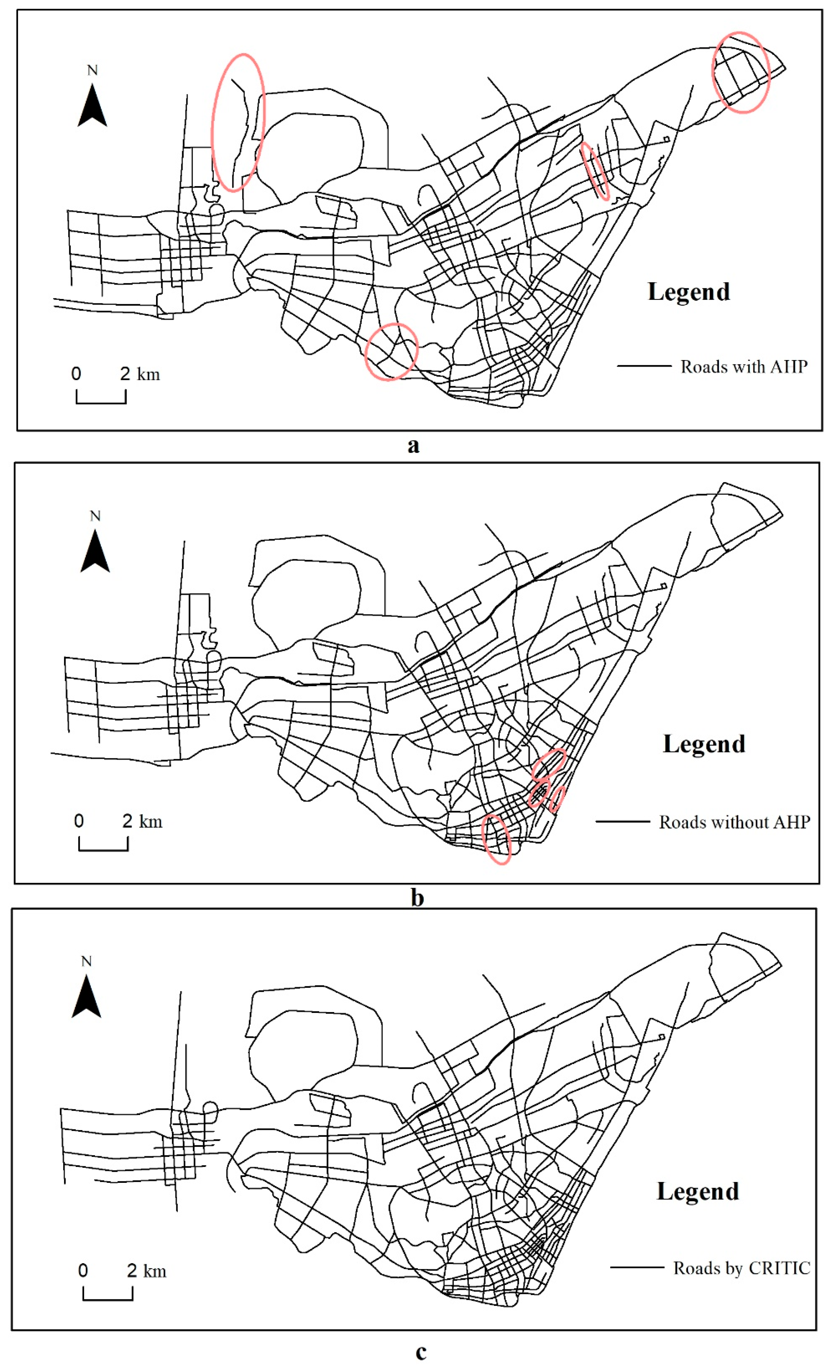
Figure 7 shows the results at a scale of 1:200,000 for the three methods. Overall, the results in Figure 7a,b are rather similar. However, after zooming into the details, a few differences can be identified. As shown in the pink circles in (a) and (b), without AHP, more strokes in the urban areas are retained, while the strokes in sub-urban are unduly eliminated. However, the strokes with significant geometric characteristics in sub-urban areas are retained with AHP. In Figure 7c, it can be observed that neither the density distribution nor the coverage of the original road network is maintained by the CRITIC method. Too much weight is assigned to the indicator of and , thus interfering with the structural characteristics of the road network. By comparing the values of the indicators in pairs and then combining the scores of the two layers, AHP achieves a more thorough and clear analysis of the relevant indicators, and accurately understands their internal relationships, thereby obtaining a more reasonable outcome.
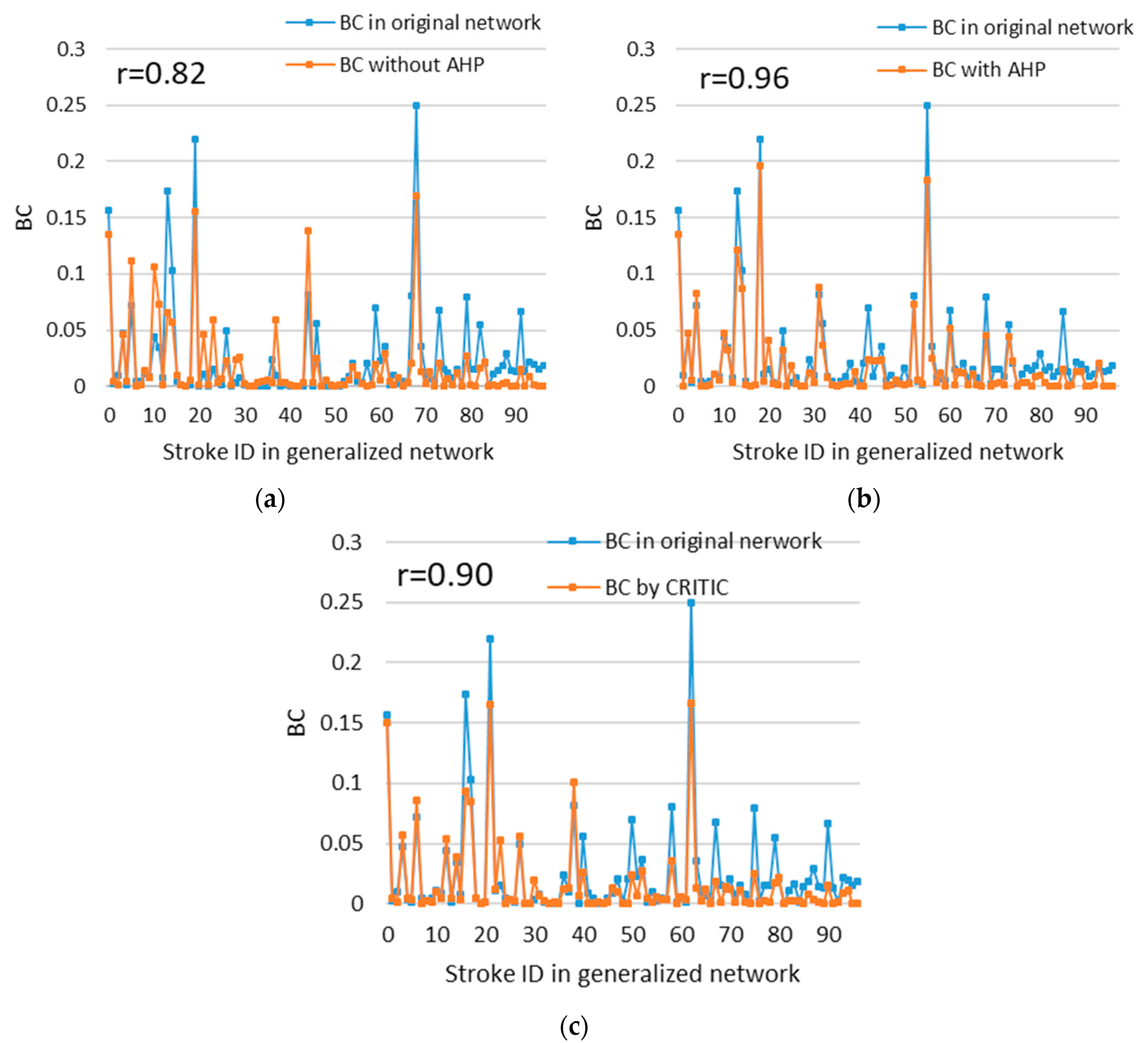
In addition to the visual evaluation, we conducted a quantitative evaluation using the Pearson correlation coefficient, which is a linear correlation coefficient ranging from -1 to 1. This coefficient is used to reflect the degree of linear correlation between two variables. The larger the absolute value, the stronger the correlation. The Pearson correlation coefficient has been used to measure the structural similarity of complex networks [23,40]. We calculated the Pearson correlation coefficient of between the generalized road networks and the original network to indicate their structural similarity. Assume that and are the node sets of network and , respectively. Then, the structural similarity between and is calculated by the following formula:
where is the similarity measure of network and ; means that the node set is shared by network and ; and both and are topological measures (that refer to the betweenness centrality in this experiment) used to measure the structural similarity of network and . and is the mean of the topological measures of and , respectively.
Figure 8 shows the statistics of the betweenness centrality of the strokes in the generalized networks and in the original network. By comparing the Pearson correlation coefficient , it can be concluded that our method better preserves the structural characteristics of the original road network.
6.2. Changes after Considering Contextual Characteristics
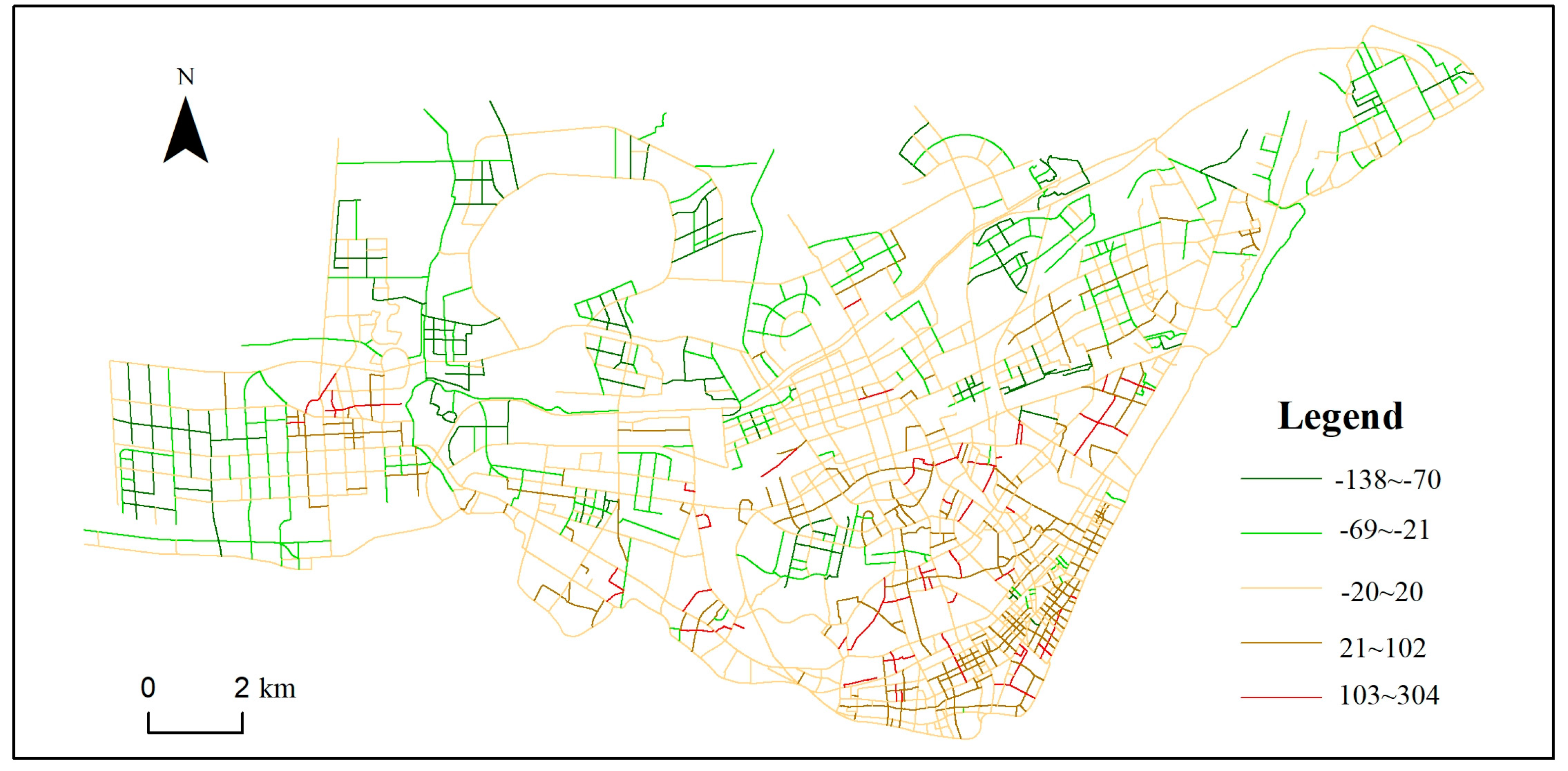
Figure 9 illustrates the changes in the importance order of the strokes after integrating the contextual characteristic indicator, in which the positive values represent an ascension in the ranking, and not vice versa. This analysis shows that the categories and number of POIs around different strokes varied, and different degrees of changes occurred in their rankings. The rankings of many streets that were insignificant in their contextual characteristics thus improved. These streets are distributed mainly in the business district at the lower-right corner of the map. However, in the suburban areas with a sparse POI distribution, there was a general drop in stroke rankings.
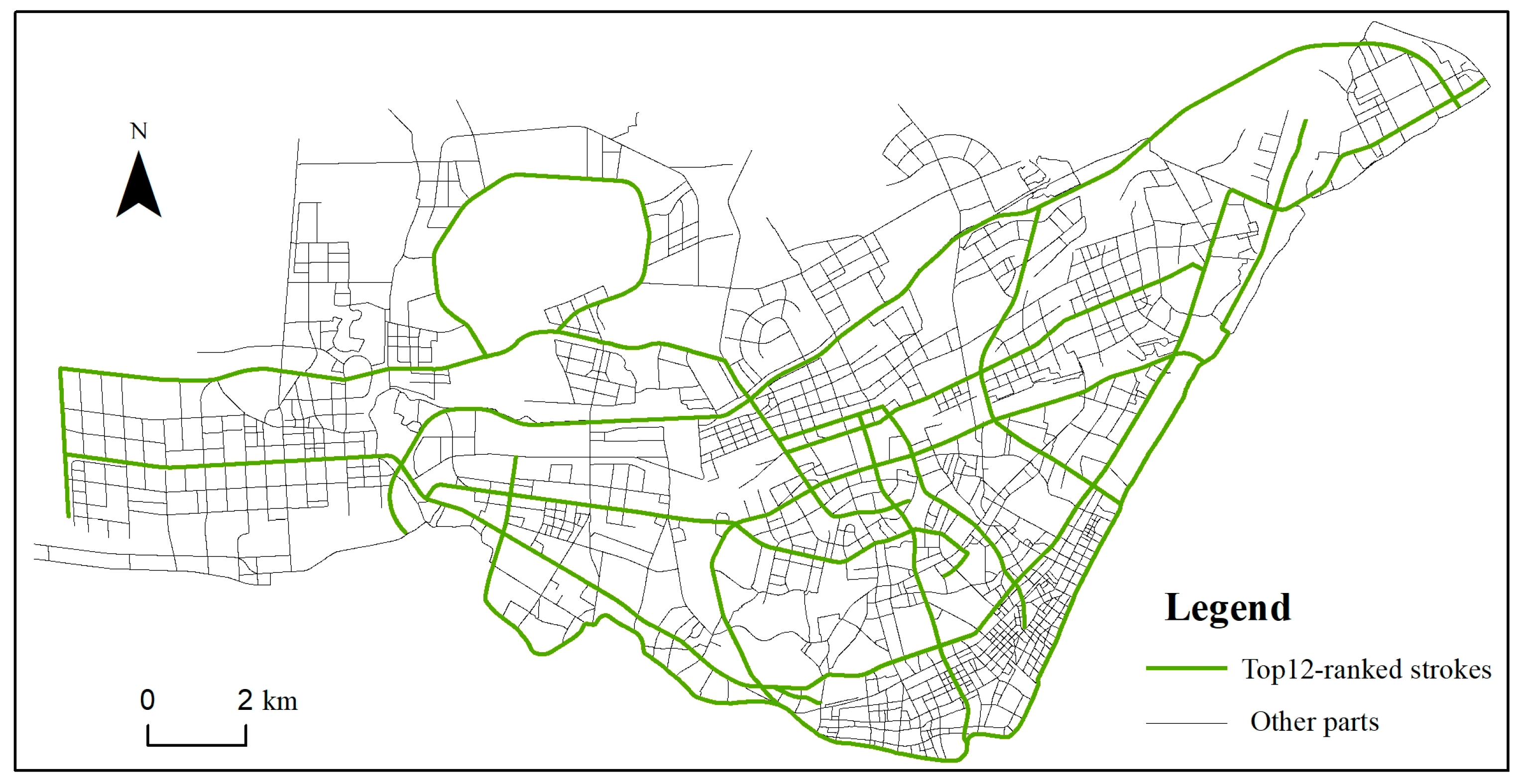
We ranked the strokes in the original network in descending order according to their values. The top twelve strokes (rendered in green in Figure 10) did not change significantly before and after the constraint of POIs, and their statistics are listed in Table 6. As indicated by their values in the table, these strokes have prominent advantages in the topological structure of the original road network. The constraint of POIs did not significantly influence their rankings. Thus, it can be concluded that our method can also preserve the main structure of the road network in the Hankou District.
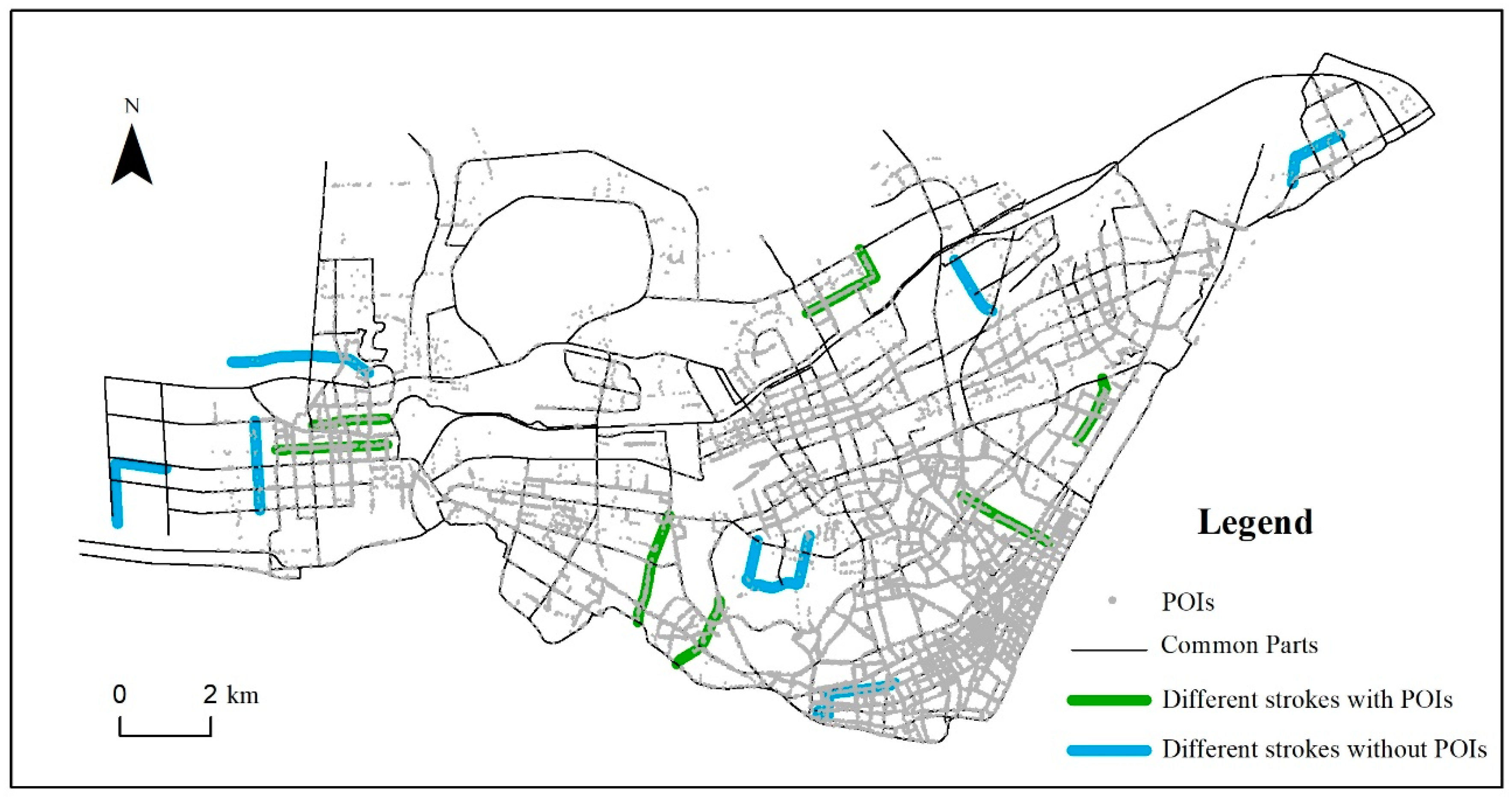
In addition, we compared the generalized results at a scale of 1:200,000 with and without the constraint of POIs. In this link, we determined the adaptive thresholds for stroke importance and the connectivity maintenance solution. The different strokes are highlighted in Figure 11. One can see that these different strokes feature similar structural characteristics. The strokes rendered in green tend to be surrounded by more POIs compared to strokes rendered in blue. These green strokes play a relatively significant role in people’s travel due to their adjacent POIs, so they should be preferentially retained in generalized maps compared to blue strokes. Therefore, roads with relatively significant contextual characteristics were selected prior to their competitors, thereby yielding a more reasonable result.
6.3. Comparison with Manual Method
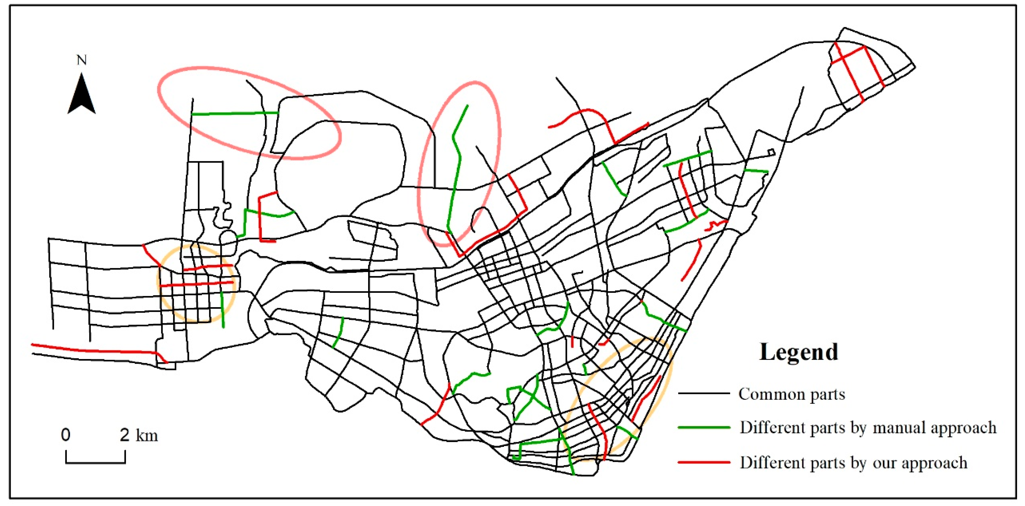
Finally, manual selection was conducted by referring to compilation specifications for national scale maps. Experienced cartographers were invited to select strokes according to general principles, to ensure the preservation of significant roads, to maintain the connection between roads and residential areas, and to maintain the characteristics of the plane graphics of road networks. The result of manual selection was treated as the benchmark. The comparison results between manual approach and our approach are shown in Figure 12. The first observation in the comparison maps is that the results of our approach basically agree with those of the manual approach.
Through in-depth discussion with our cartographic experts, we evaluated the generalized results of our method as follows: The general thinning of the road network was acceptable. The road networks in urban and sub-urban areas were properly generalized overall. However, slight thinning was still needed in denser areas (in the orange circles). Some roads (in the pink circles) that reflected significant structural features of the network were pruned. The ‘crisp boundary effect’, the adaptive thresholds, the constraint of POIs, or the lack of road class are potential reasons for these deviations.
To reflect the results more specifically, we adopted the maximum similarity approach to measure the consistency among two results. The similarity results are listed in Table 7. The statistics indicate that the two results achieve good consistency.
7. Conclusions
The accurate and reasonable evaluation of roads is a prerequisite for road selection. Some weighting methods such as CRITIC, entropy, and coefficient of variation are widely used in line-based methods. The weights of the road indicators assigned by these methods are not consistent with actual cartographic experience. In this regard, we adapted AHP to prioritize our strokes. Among the various road selection methods, line-based methods generally include multiple indicators to determine the priority order of roads, which can be deemed a multi-attribute decision-making problem. Considering the advantages of AHP in handling this kind of problem, a new road selection method is proposed based on AHP. Previous studies tend to solely rely on the indicators summarized by the intrinsic information of road networks. However, if the effects of other features, such as surrounding habitations or facilities, are included and quantitatively described in the selection method, the produced road network might be more in tune with actual needs. Therefore, we established a road evaluation indicator system that considers both the structural and contextual characteristics of roads. In our method, the contextual characteristic indicator is built according to the surrounding POIs of roads, which is then integrated into the model of AHP along with structural characteristic indicators to calculate the importance values of strokes. We also designed another two complementary solutions, namely preset adaptive thresholds and connectivity maintenance, to improve the generalized results.
To evaluate the performance, we carried out visual and quantitative experiments. Some improvements in terms of the structures and contextual characteristics of roads could be identified. The results ofour method achieved higher accuracy than manual selection. Hence, it is feasible to apply AHP to road selection. In addition, the extra computing time produced by the proposed indicator in Section 3.3.2 can be ignored. Thus, this method has the potential to be adopted in road generalization.
Author Contributions
Z.W. helped conceive and design the study; Y.H. carried out the method and wrote the manuscript; X.L. and B.H. offered significant contribution to result evaluation; All authors have read and agreed to the published version of the manuscript.
Funding
This research was funded by National Natural Science Foundation of China (No. 41561090,41861060 and 41930101), The Project Supported by the Open Fund of Key Laboratory of Urban Land Resources Monitoring and Simulation, Ministry of Land and Resources (No. KF-2018-03-007), LZJTU EP (No. 201806) as well as Youth Program of National Natural Science Foundation of China(No.41801395).
Acknowledgments
We sincerely appreciate the Editor’s encouragement and the anonymous reviewer’s valuable support.
Conflicts of Interest
The authors declare that they have no conflict of interest.
References
- Chen, B.; Wu, F.; Qian, H.Z. Study on Road Networks Auto-selection Algorithms. J. Image Gr. 2008, 13, 2388–2393. [Google Scholar] [CrossRef]
- Yang, M.; AI, T.H.; Zhou, Q. A Method of Road Network Generalization Considering Stroke Properties of Road Object. Acta Geod. Cartogr. Sin. 2013, 42, 581–587. [Google Scholar]
- Mackaness, W. Analysis of Urban Road Networks to Support Cartographic Generalization. Cartogr. Geogr. Inf. Sci. 1995, 22, 306–316. [Google Scholar] [CrossRef]
- Jiang, B.; Claramunt, C. A Structural Approach to the Model Generalization of an Urban Street Network*. GeoInformatica 2004, 8, 157–171. [Google Scholar] [CrossRef]
- Hu, Y.G.; Chen, J.; Li, Z.L. Selective Omission of Road Features Based on Mesh Density for Digital Map Generalization. Acta Geod. Cartogr. Sin. 2007, 36, 351–357. [Google Scholar] [CrossRef]
- Li, Z.; Zhou, Q. Integration of linear and areal hierarchies for continuous multi-scale representation of road networks. Int. J. Geogr. Inf. Sci. 2012, 26, 855–880. [Google Scholar] [CrossRef]
- Peng, W.N.; Muller, J.C. A Dynamic Decision Tree Structure Supporting Urban Road Network Automated Generalization. Cartogr. J. 1996, 33, 5–10. [Google Scholar] [CrossRef]
- Edwardes, A.J.; Mackaness, W.A. Intelligent Generalization of Urban Road Networks. In Proceedings of the GIS Research UK Conference, New York, NY, USA, January 2000. [Google Scholar]
- Deng, H.Y.; Wu, F.; Wang, H.L. A Generalization of Road Networks Based on Topological Similarity. J. Geomat. Sci. Technol. 2008, 25, 183–187. [Google Scholar]
- Chen, J.; Hu, Y.; Li, Z.; Zhao, R.; Meng, L. Selective omission of road features based on mesh density for automatic map generalization. Int. J. Geogr. Inf. Sci. 2009, 23, 1013–1032. [Google Scholar] [CrossRef]
- Touya, G. A Road Network Selection Process Based on Data Enrichment and Structure Detection. Trans. GIS 2010, 14, 595–614. [Google Scholar] [CrossRef] [Green Version]
- Thomson, R.C.; Richardson, D.E. A Graph Theory Approach to Road Network Generalization. In Proceedings of the 17th International Cartographic Conference, Barcelona, Spain, 3–9 September 1995; pp. 1871–1880. [Google Scholar]
- Weiss, R.; Weibel, R. Road network selection for small-scale maps using an improved centrality-based algorithm. J. Spat. Inf. Sci. 2014, 9, 71–99. [Google Scholar] [CrossRef]
- Liu, X.; Zhan, F.B.; Ai, T. Road selection based on Voronoi diagrams and “strokes” in map generalization. Int. J. Appl. Earth Obs. Geoinf. 2010, 12, S194–S202. [Google Scholar] [CrossRef]
- Thomson, R.C.; Richardson, D.E. The Good Continuation Principle of Perceptual Organisation Applied to the Generalisation of Road Networks. In Proceedings of the 19th International Cartographic Conference, Ottawa, ON, Canada, 14–21 August 1999; pp. 1215–1223. [Google Scholar]
- Zhang, Q.N. Road Network Generalization Based on Connection Analysis. In Proceedings of the 11th International Symposium on Spatial Data Handling, Leicester, UK, 22–24 August 2004. [Google Scholar] [CrossRef]
- Tian, J.; Luo, Y.; Lin, L.P. A Comparative Study of Two Strategies of Road Network Selection. Geomat. Inf. Sci. Wuhan Univ. 2019, 44, 310–316. [Google Scholar] [CrossRef]
- Yang, B.; Luan, X.; Li, Q. Generating hierarchical strokes from urban street networks based on spatial pattern recognition. Int. J. Geogr. Inf. Sci. 2011, 25, 2025–2050. [Google Scholar] [CrossRef]
- Xu, Z.; Liu, C.; Zhang, H. Road Selection Based on Evaluation of Stroke Network Functionality. Acta Geod. Cartogr. Sin. 2012, 41, 769–776. [Google Scholar]
- Richardson, D.E.; Thomson, R.C. Integrating Thematic, Geometric, and Topologic Information in the Generalization of Road Networks. Cartographica 1996, 33, 75–83. [Google Scholar] [CrossRef]
- Deng, H.G.; Wu, F.; Zhai, R.J. A Generalization Model of Road Networks Based on Genetic Algorithm. Geomat. Inf. Sci. Wuhan Univ. 2006, 31, 164–167. [Google Scholar] [CrossRef]
- Xu, Z.B.; Wang, Z.H.; Yan, H.W. A Method for Automatic Road Selection Combined with POI Data. J. Geo-Inf. Sci. 2018, 20, 159–166. [Google Scholar]
- Song, H.Q.; Guo, J.; Liu, G. Auto Generalization Approach and Importance Evaluation of Urban Roads Based on Complex Networks. Eng. Surv. Map. 2017, 26, 8–12. [Google Scholar]
- Cao, W.W.; Zhang, H. Road Selection Considering Structural and Geometric Properties. Geomat. Inf. Sci. Wuhan Univ. 2017, 42, 520–524. [Google Scholar]
- Benz, S.A.; Weibel, R. Road network selection for medium scales using an extended stroke-mesh combination algorithm. Cartogr. Geogr. Inf. Sci. 2014, 41, 323–339. [Google Scholar] [CrossRef] [Green Version]
- Zhang, J.; Wang, Y.; Zhao, W. An Improved Hybrid Method for Enhanced Road Feature Selection in Map Generalization. ISPRS Int. J. Geo-Inf. 2017, 6, 196. [Google Scholar] [CrossRef] [Green Version]
- Yu, W.; Zhang, Y.; Ai, T.; Guan, Q.; Chen, Z.; Li, H. Road network generalization considering traffic flow patterns. Int. J. Geogr. Inf. Sci. 2019, 34, 119–149. [Google Scholar] [CrossRef]
- Luan, X.C.; Yang, B.S.; Zhang, Y.F. Structural Hierarchy Analysis of Streets Based on Complex Network Theory. Geomat. Inf. Sci. Wuhan Univ. 2012, 37, 728–732. [Google Scholar] [CrossRef]
- Saaty, T.L. What is the analytic hierarchy process. In Mathematical Models for Decision Support; Springer: Berlin/Heidelberg, Germany, 1988; pp. 109–121. [Google Scholar]
- Vaidya, O.S.; Kumar, S. Analytic hierarchy process: An overview of applications. Eur. J. Oper. Res. 2006, 169, 1–29. [Google Scholar] [CrossRef]
- Jiang, B.; Liu, C. Street-based topological representations and analyses for predicting traffic flow in GIS. Int. J. Geogr. Inf. Sci. 2009, 23, 1119–1137. [Google Scholar] [CrossRef] [Green Version]
- Zhao, G.F.; Yuan, S.W.; Yusheng, C. Analysis of Complex Network Property and Robustness of Urban Road Network. J. Hwy. Trans. Res. Dvpt. 2016, 33, 119–124. [Google Scholar]
- Zhou, Q.; Li, Z. A comparative study of various strategies to concatenate road segments into strokes for map generalization. Int. J. Geogr. Inf. Sci. 2012, 26, 691–715. [Google Scholar] [CrossRef]
- Zhang, Y.F.; Yang, B.S.; Luan, X.C. Integrating Urban POI and Road Networks Based on Semantic Knowledge. Geomat. Inf. Sci. Wuhan Univ. 2013, 38, 1229–1233. [Google Scholar] [CrossRef]
- Hu, H.M.; Qian, H.Z. Auto-selection of areal Habitation Based on Analytic Hierarchy Process. Acta Geod. Cartogr. Sin. 2016, 45, 740–746. [Google Scholar] [CrossRef]
- Hsu, C.C.; Sandford, B.A. The Delphi technique: making sense of consensus. Pract. Ass. Res. Eval. 2007, 12, 1–8. [Google Scholar]
- Tian, J.; Xiong, F.Q. Road Density Partition and Its Application in Evaluation of Road Selection. Geomat. Inf. Sci. Wuhan Univ. 2016, 41, 1225–1231. [Google Scholar] [CrossRef]
- Sujit, K.S.; Martin, B. Geospatial Analysis of Building Structures in Megacity Dhaka: The Use of Spatial Statistics for Promoting Data-driven Decision-making. J. Geo-visu. Spat. Ann. 2019, 3, 7. [Google Scholar]
- Namtirtha, A.; Dutta, A.; Dutta, B. Weighted kshell degree neighborhood method: An approach independent of completeness of global network structure for identifying the influential spreaders. In Proceedings of the 10th International Conference on Communication Systems & Networks (COMSNETS), Bangalore, India, 3–7 January 2018; pp. 81–88. [Google Scholar] [CrossRef]
- Lü, L.; Medo, M.; Yeung, C.H.; Zhang, Y.-C.; Zhang, Z.-K.; Zhou, T. Recommender systems. Phys. Rep. 2012, 519, 1–49. [Google Scholar] [CrossRef] [Green Version]
Figure 1.
Original road network of the Hankou district and the distribution of POIs inside the road buffer.
Figure 1.
Original road network of the Hankou district and the distribution of POIs inside the road buffer.

Figure 2.
Two types of representations for a road network.

Figure 3.
Analytic hierarchy model of strokes importance.

Figure 4.
Road density partition result and the preset thresholds of the clustered regions. Denser areas are constrained by more stringent thresholds.
Figure 4.
Road density partition result and the preset thresholds of the clustered regions. Denser areas are constrained by more stringent thresholds.

Figure 5.
Process of road selection.

Figure 6.
Connectivity maintenance of the selected strokes.

Figure 7.
Generalized road networks with AHP (a), without AHP (b), and by CRITIC (c).

Figure 8.
The statistics of the values of the selected roads before and after the three selection processes: (a) The values of the selected roads without AHP; (b) the values of the selected roads with AHP; (c) the values of the selected roads using the CRITIC. The Pearson correlation coefficient reveals the similarity of the topological characteristics between the generalized results and the original road network.

Figure 9.
Changes in the order of strokes before and after the constraint of POIs.

Figure 10.
Twelve strokes with the highest values in the original road network.

Figure 11.
Comparison between the results with and without the constraint of POIs. The green strokes tend to be surrounded by more POIs, compared to blue strokes, indicating that our method can preserve more roads with relatively significant contextual characteristics.
Figure 11.
Comparison between the results with and without the constraint of POIs. The green strokes tend to be surrounded by more POIs, compared to blue strokes, indicating that our method can preserve more roads with relatively significant contextual characteristics.

Figure 12.
Comparison between our method and manual method. Our method is still unable to reach desired effects in all aspects due to some non-optimal parts of the method. Slight thinning was needed in denser areas (in the orange circles). Some roads (in the pink circles) that reflected significant structural features of the network were pruned.


Table 1.
Numerical scale of relative importance.
| Numerical Scale | Interpretation |
|---|---|
| 1 | Equally important |
| 3 | Weakly important |
| 5 | Moderately important |
| 7 | Very important |
| 9 | Extremely important |
| 2, 4, 6, 8 | In between their two neighbors |
Table 2.
Mean random consistency index.
| 1 | 2 | 3 | 4 | 5 | 6 | 7 | 8 | 9 | |
|---|---|---|---|---|---|---|---|---|---|
| RI | 0 | 0 | 0.58 | 0.90 | 1.12 | 1.24 | 1.32 | 1.41 | 1.45 |
Table 3.
Reclassification of Points of Interest (POIs).
| First Class Classification | Second Class Classification |
|---|---|
| Residence Communities | residential areas, villas, etc. |
| Public Management | government agencies and administrative offices |
| Public Services | medical care, science and education, life services, etc. |
| Business Services | catering services, shopping services, financial services, accommodation services, etc. |
| Industrial | factories |
| Logistics and warehousing | warehouses, postal services, etc. |
| Transportation | transport facilities, affiliated facilities of roads, etc. |
| Public facilities | power supply, sewage treatments, public toilets, etc. |
| Greenbelts and squares | parks, squares, etc. |
Table 4.
Scores of partial POI categories.
| First Class Classification | Third Class Classification | Scores |
|---|---|---|
| Residence Communities | residential districts | 1.25 |
| Public Management | provincial and municipal government agencies | 4.75 |
| Public Services | art troupes | 1 |
| general hospitals | 4.875 | |
| movie theaters | 1.375 | |
| sports venues | 1 | |
| national attractions | 4.625 | |
| research institutions | 3.625 | |
| Business Services | supermarkets | 4.5 |
| four-star hotels | 2.125 | |
| hostels | 1 | |
| office buildings | 1 | |
| Industrial | mining companies | 1.125 |
| Logistics and warehousing | postal offices | 1.625 |
| Transportation | railway stations | 4.25 |
| subways | 2 | |
| Public facilities | public toilets | 1 |
| Greenbelts and squares | zoos | 2.75 |
Table 5.
Comparison matrix of the indicators.
| 1 | 2 | 2 | 2 | |
| 1/2 | 1 | 1 | 1 | |
| 1/2 | 1 | 1 | 1 | |
| 1/2 | 1 | 1 | 1 |
Table 6.
Changes in the order of the top twelve-ranked strokes.
| Stroke ID | Order without POI | Order with POI | Difference in Order | ||||
|---|---|---|---|---|---|---|---|
| 0 | 2 | 2 | 0 | 0.15 | 30,224.67 | 1849.5 | 64 |
| 13 | 10 | 9 | 1 | 0.07 | 7256.21 | 1063.25 | 30 |
| 37 | 3 | 3 | 0 | 0.17 | 17,041.61 | 1866 | 53 |
| 39 | 5 | 4 | 1 | 0.10 | 14,541.79 | 941.25 | 35 |
| 52 | 1 | 1 | 0 | 0.21 | 21,111.06 | 1945.25 | 65 |
| 104 | 6 | 6 | 0 | 0.08 | 7887.87 | 1407.62 | 34 |
| 163 | 8 | 7 | 1 | 0.07 | 12,463.45 | 1388.88 | 41 |
| 220 | 4 | 5 | −1 | 0.08 | 26,758.73 | 347.625 | 22 |
| 247 | 0 | 0 | 0 | 0.24 | 22,525.28 | 332.375 | 46 |
| 282 | 11 | 12 | −1 | 0.06 | 7766.20 | 187.375 | 25 |
| 346 | 7 | 8 | −1 | 0.07 | 9474.87 | 809.375 | 29 |
| 478 | 9 | 11 | −2 | 0.06 | 11,430.17 | 67.375 | 21 |
Table 7.
Statistics of maximum similarity and its related parameters.
| Parameters | Values |
|---|---|
| Total length of roads by manual method /km | 560,498.1 |
| Total length of roads by our method /km | 534,801 |
| Total length of common roads of two methods /km | 522,549.5 |
| Maximum Similarity | 0.91 |
| Ratio of common stroke number among two methods to total selected number | 0.89 |
© 2020 by the authors. Licensee MDPI, Basel, Switzerland. This article is an open access article distributed under the terms and conditions of the Creative Commons Attribution (CC BY) license (http://creativecommons.org/licenses/by/4.0/).
Share and Cite
MDPI and ACS Style
Han, Y.; Wang, Z.; Lu, X.; Hu, B. Application of AHP to Road Selection. ISPRS Int. J. Geo-Inf. 2020, 9, 86. https://0-doi-org.brum.beds.ac.uk/10.3390/ijgi9020086
AMA Style
Han Y, Wang Z, Lu X, Hu B. Application of AHP to Road Selection. ISPRS International Journal of Geo-Information. 2020; 9(2):86. https://0-doi-org.brum.beds.ac.uk/10.3390/ijgi9020086
Chicago/Turabian StyleHan, Yuan, Zhonghui Wang, Xiaomin Lu, and Bowei Hu. 2020. "Application of AHP to Road Selection" ISPRS International Journal of Geo-Information 9, no. 2: 86. https://0-doi-org.brum.beds.ac.uk/10.3390/ijgi9020086
Note that from the first issue of 2016, this journal uses article numbers instead of page numbers. See further details here.