Machine Learning Generalisation across Different 3D Architectural Heritage


3D Optical Metrology (3DOM) unit, Bruno Kessler Foundation (FBK), Via Sommarive 18, 38121 Trento, Italy
*
Author to whom correspondence should be addressed.
ISPRS Int. J. Geo-Inf. 2020, 9(6), 379; https://0-doi-org.brum.beds.ac.uk/10.3390/ijgi9060379
Submission received: 28 April 2020
/
Revised: 28 May 2020
/
Accepted: 5 June 2020
/
Published: 9 June 2020
(This article belongs to the Special Issue Automatic Feature Recognition from Point Clouds)
Abstract
:The use of machine learning techniques for point cloud classification has been investigated extensively in the last decade in the geospatial community, while in the cultural heritage field it has only recently started to be explored. The high complexity and heterogeneity of 3D heritage data, the diversity of the possible scenarios, and the different classification purposes that each case study might present, makes it difficult to realise a large training dataset for learning purposes. An important practical issue that has not been explored yet, is the application of a single machine learning model across large and different architectural datasets. This paper tackles this issue presenting a methodology able to successfully generalise to unseen scenarios a random forest model trained on a specific dataset. This is achieved looking for the best features suitable to identify the classes of interest (e.g., wall, windows, roof and columns).
1. Introduction
The documentation, restoration and conservation of architectural heritage monuments have become fundamental for protecting and preserving them from armed conflicts, climate change effects, natural catastrophes and human-caused disasters. The presence of these risks is further enlarged by the fact that all monuments are inevitably in a constant state of chemical transformation.
The advent in the last decades of 3D optical instruments for the 3D digitisation of objects and sites has undoubtedly changed the concept of heritage conservation and preservation. Indeed, the cultural heritage (CH) field is taking great advantage of reality-based surveying techniques (e.g., photogrammetry, laser scanning) [1,2]. Currently, digital photogrammetry and laser scanning have become standard methods for data acquisition and digital recording for the 3D documentation of heritage assets. These technologies for 3D documentation allow the generation of realistic 3D results in terms of geometric and radiometric accuracy, overcoming the so-called direct surveys, which involve measuring in direct contact of objects or excavation areas. Once data are acquired (images, scans, single points, etc.), post-processing operations allow the derivation of dense point clouds, polygonal models, orthoimages, sections, maps and drawing or further products. Towards providing precise representations of the objects at a given time to be passed down to future generations, these kinds of data can be used as a base for any further studies [3]. In this context, the association of semantic information to the point clouds leads to a simplification in the CH reading, accelerating the phase of data management and interpretation. There are various applications where semantically annotated point clouds are requested such as:
As most of these applications are based on time-consuming and subjective manual procedures of annotation, it becomes fundamental to realise a more objective and automated classification method.
1.1. State of the Art
Up to now, machine- and its subset deep-learning algorithms (ML / DL) have become the state-of-the-art method to deal with point cloud classification, overcoming rule-based approaches such as Hough transform, Random Sample Consensus (RANSAC), or region growing, presented by Grilli et al. in [19]. Among the ML approaches, the studies proposed in Vosselman [20], Weinmann et al. [21], and Niemeyer et al. [22] can be considered as pioneer works in the geospatial field. Equally, on the DL side, it is fundamental to mention PointNet and its later improvement PointNet++ [23,24], built to perform the classification/part segmentation of simple objects with replicated shapes (e.g., mug, plane, table, car). Both ML and DL are fields of artificial intelligence scientific research related to the development of algorithms that allow computers to make predictions based on empirical training data. Associated with the training data are the so-called features, variables found in the given training set, that can powerfully or at least sufficiently help us at building an accurate predictive model. While within standard machine learning approaches, the choice of the features depends on the operators, deep-learning methods can learn the features by themselves, as part of the training process [25]. This ability to learn features is considered as one of the main causes for the quick advance in 2D and 3D understanding benchmark results [26]. However, deep learning does so using neural networks with many hidden layers, powerful computational resources and a significant amount of annotated data [27]. In this regard, the availability/unavailability of data can raise/limit the application of the deep-learning approaches in some fields more than in other ones. As Griffith and Boehm asserted [26], benchmarks are essential to provide the community with high-quality training data, also allowing a fair comparison between the various algorithms/approaches.
Although current public datasets provide several indoor [28,29,30] and outdoor scenes [31,32,33,34], there is still an evident lack of benchmarks designed for the heritage and architectural field. Despite this, in recent years the following solutions have been proposed. A random forest (RF) classifier has been used on texture and geometric data in [35]. Murtiyoso and Grussenmeyer [36] have proposed an algorithmic approach to perform point cloud segmentation through geometric rules and mathematical functions. Pierdicca et al. [37] presented a dynamic graph convolutional neural network (DGCNN) for point cloud segmentation trained with 11 labelled scenes of heritage architecture.
1.2. Aim and Contribution of the Paper
The design of a heritage data classification model is challenging due to the high variability of scenarios in this field. In addition, the class definition might change according to the classification aims (e.g., architectural element identification vs. material quantification) and the case study treated (e.g., classic temples differ from churches, churches can differ a lot from each other according to their architectural style, etc.).
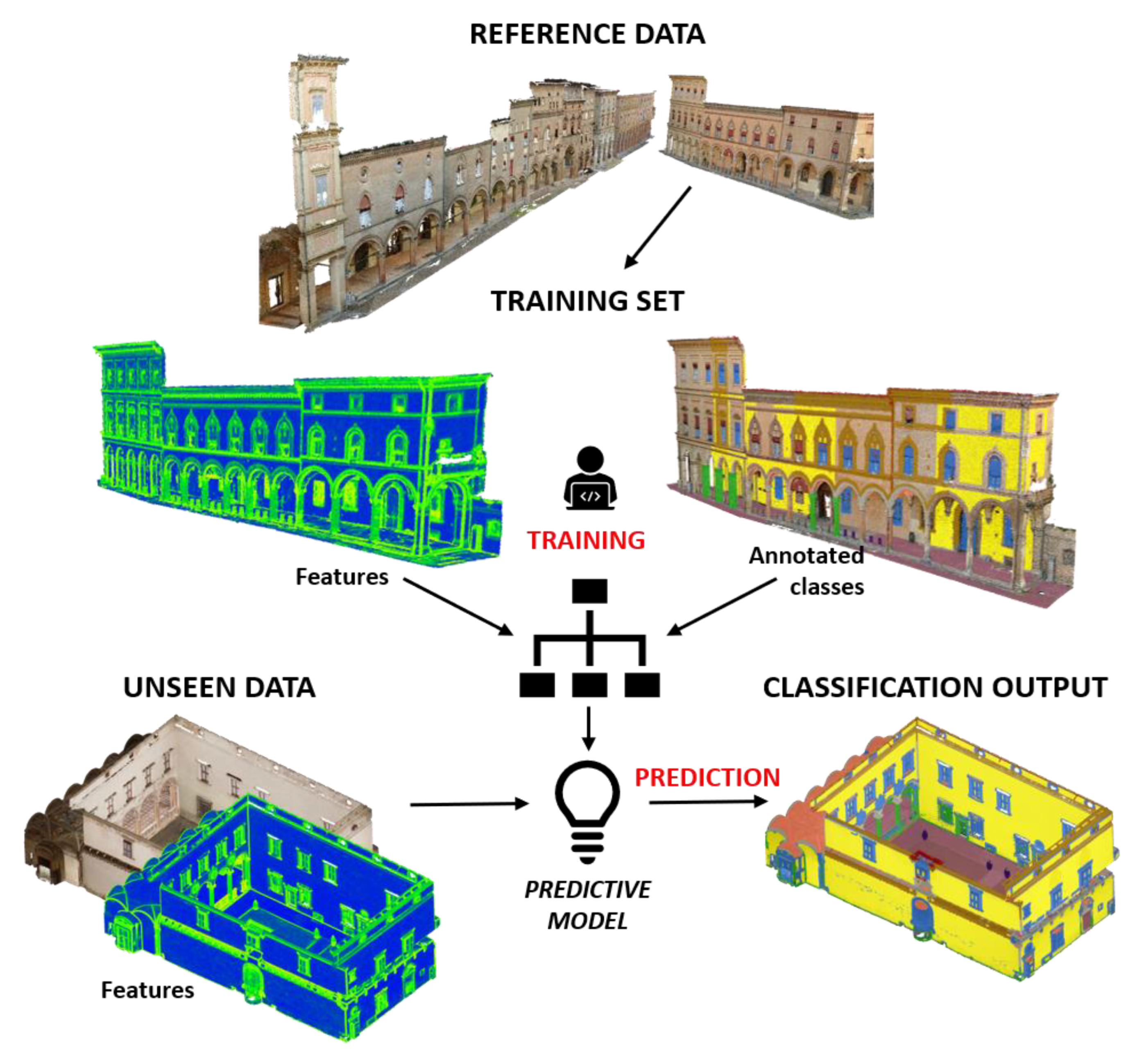
In our previous work [38], a standard machine learning approach based on an accurate selection of geometric features was developed to facilitate and accelerate the classification of some heritage monuments. While before, for each case study a specific model was trained (Figure 1), the main aim of this paper is to verify the capability of a pre-trained model to generalise over other unseen 3D scenarios, featuring similar characteristics (Section 2). When we talk about ‘generalisation’, we refer to a machine learning model’s ability to perform well on new, unseen data, rather than just the data that it was trained on. This term might be confused with the concept of ‘transfer learning’, used in the deep learning community to indicate the use of a model pre-trained for a particular task to solve a different problem (i.e., using a model trained to recognise apples for identifying pears) [39,40]. In order to test the generalisation concept, we worked with urban architectures (Section 1.3), looking for some recurrent classes such as floors, facades, windows, doors and columns. (Figure 2).
An additional goal of this work is to test the generalisation when training and test datasets are acquired with different sensors (i.e., terrestrial photogrammetry and terrestrial laser scanners), featuring different resolutions, levels of noise, and attributes (Section 3.2).
In summary, the aims and contributions of the presented work are:
- Identifying a set of transversal architectural classes and a few (geometric and radiometric) features that can behave similarly among different datasets;
- Generalising a pre-trained random forest (RF) classifier over unseen 3D scenarios, featuring similar characteristics;
- Classifying 3D point clouds featuring different characteristics, in terms of acquisition technique, geometric resolution and size.
In the next paragraph, the heritage datasets used for the experiments are presented. In Section 2 the adopted approach is described, with particular regard to the identification of the classes and the feature selection. Section 3 presents different experiments and discusses the classification results, followed by the conclusions in Section 4.
1.3. Datasets
The different datasets used in our experiments consist of five photogrammetric point clouds provided with RGB colour information and one laser scanned point cloud without colour information (Table 1).
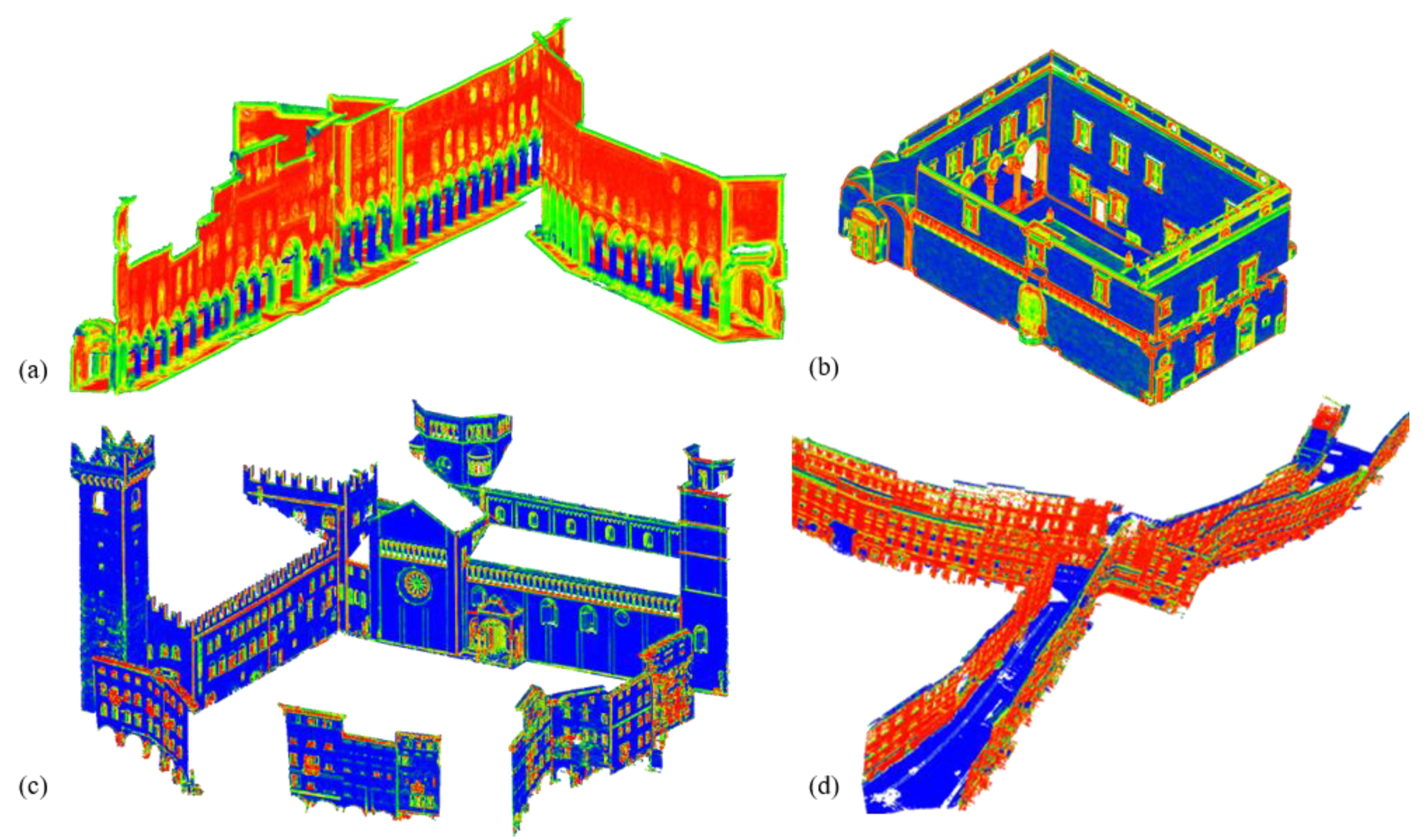
The first three datasets considered (Table 1 - A–B–C) represent a portion of the 40 km of porticoes built between the 11th–20th centuries in Bologna. As they became a distinctive building feature of the city, 25% of the porticoes were digitised using terrestrial photogrammetry under a project for the candidature of the porticoes as UNESCO “world heritage site” [41]. Such structures are interesting for our study, because they combine various types of columns and vaults, different materials, and many architectural details such as mouldings and ornaments. Among them, the Bologna–S. Stefano dataset (Table 1 - A) was considered as a reference dataset where some portions were annotated and used as a training set. This dataset was chosen because it represents a heterogeneous starting point for the subsequent classification of the other scenarios (Figure 3).
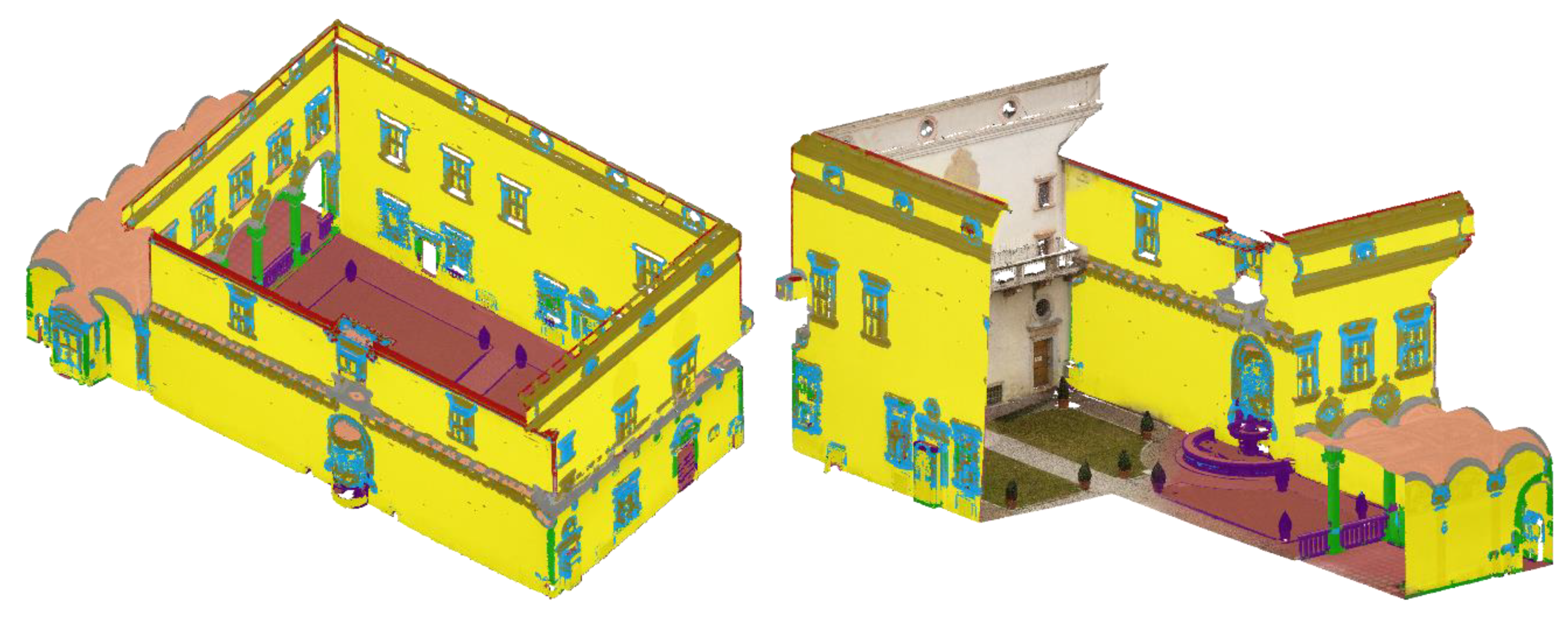
Dataset D comes from a photogrammetric survey of the Buonconsiglio Castle in Trento (Italy). It is the renaissance-style lodge of the castle (15th century) that, despite being of modest size, includes all the architectural classes previously annotated in the Bologna dataset.
To test the generalisation properties of the model we also worked on the challenging dataset of the Dome square in Trento (E), composed of buildings of different styles and periods, including the medieval praetorian palace, the city tower and the Dome (12th–13th centuries).
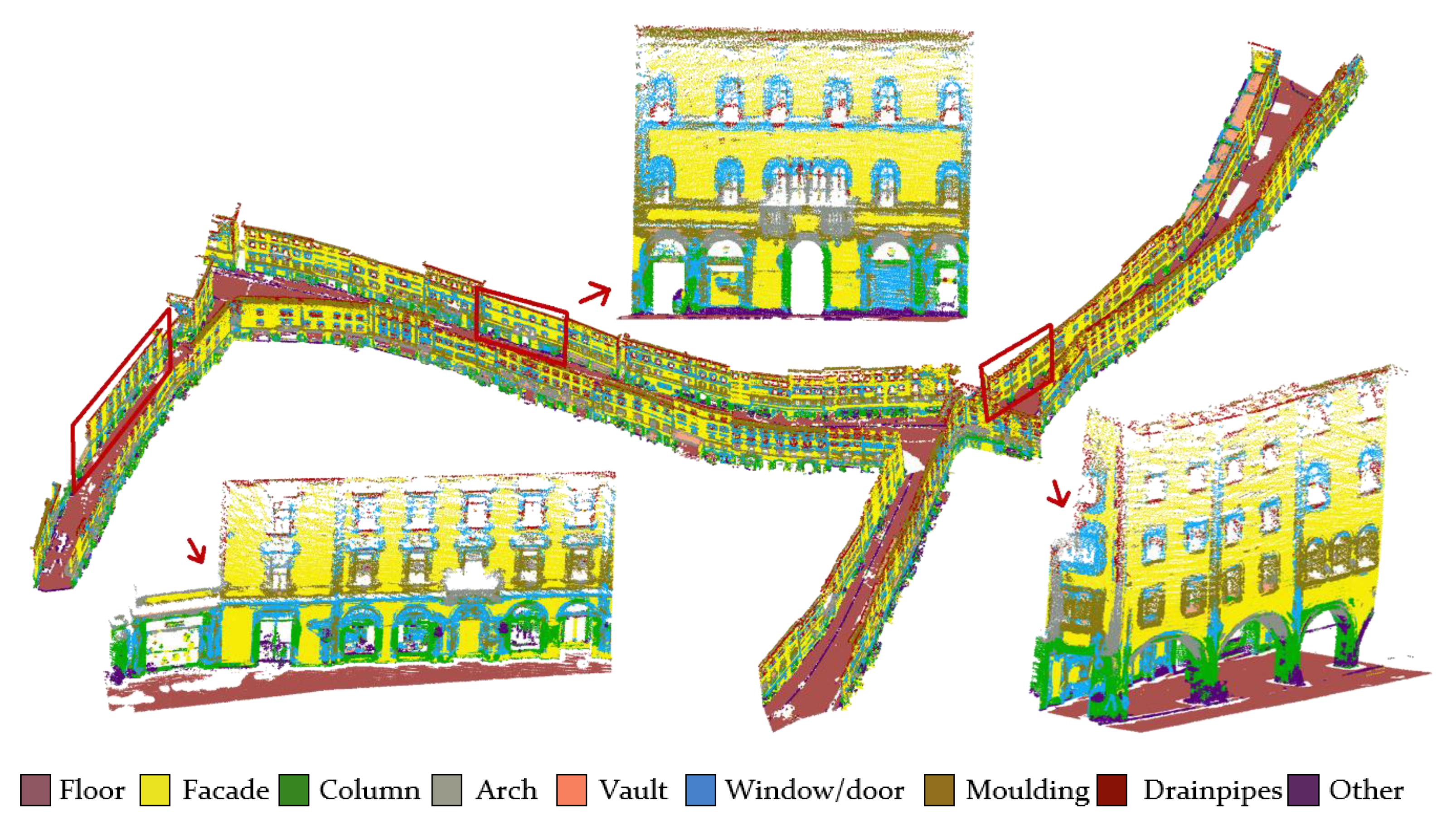
Finally, the classification was extended to a big portion of the old town of Trento (F) (about 1 km of facades), surveyed with a hand-held laser scanning system. A critical problem with this dataset was the presence of a decreasing spatial resolution from ground to top, as well as the absence of the texture information.
2. Methodology
Even considering the advent of the deep learning approaches for point cloud classification [26], in this paper we chose to work with a random forest (RF) algorithm [42], for the following reasons:
- We wanted to extend the method presented in our previous study [38], and verify its applicability to larger and different scenarios;
- There is a lack of annotated architectural training data necessary for training a neural network.
RF uses an ensemble of classification trees, then gets a prediction from each tree and selects the best solution through voting. Each tree represents an individual classifier in the ensemble and is trained on a random subset of the training sample. During the training phase, both class labels and features were given as input to the model so it can learn to classify points based on these features. In this context, to increase the reliability of the generalisation, we had to make sure that the training dataset was as representative as possible of the entire scenario. To achieve this, it was fundamental to identify (i) transversal classes (Section 2.1) and (ii) features that could behave similarly among different datasets (Section 2.2).
In our classification experiments, the Scikit-learn Python library (version 0.21.1) was used [47] to train the RF classifier and predict the classes over unseen areas.
2.1. Class Selection
For the class selection, we followed the idea proposed in [48], where classes have been defined by studying several standards and dictionaries underlying the construction of 3D architectural models. In addition to their proposed floor, facade, column, arch, vault, window and door, we decided to add the classes moulding, drainpipe and other. This last category specifically includes all those objects that do not belong to the architectural classes (e.g., low vegetation, fences, garbage cans, bikes).
2.2. Feature Selection
A critical part of the success of a classification model relies on the good selection of the training features. In order to characterise each point for classification, we combined the use of (i) radiometric and (ii) geometric features, extracted from the point clouds.
2.2.1. Radiometric Features
Radiometric features, when available, can be useful to recognise objects such as windows, commonly painted with specific colours, or also drainpipes, covered with a reflective material resulting in a high-intensity value. Given that different colour spaces represent the colour information in different ways, some of them can facilitate certain calculations [35]. Hence, after various attempts, in this work we chose to use both a composite channel of the RGB values ((R+G+B) / 3) and the colour component b* of the colour space La*b* [50]. In the L*a*b* colour space, L* indicates lightness and a* and b* are chromaticity coordinates. The a* and b* coordinates are the red/green and yellow/blue axis. Ignoring the L channel (luminance) makes the algorithm more robust to lighting differences. The colour component b* was chosen as it can facilitate the distinction between windows and walls (Figure 5).
2.2.2. Geometric Features–Covariance Features
To describe the geometric distribution of the points and highlight the discontinuities between the architectural elements, we used a few selected covariance features from [51]. The covariance features are widely used in segmentation and classification procedures because of their capability to provide in-depth knowledge on the geometrical structure of the reconstructed scene [21,52,53]. These features derive from the normalised eigenvalues λi (λ1 > λ2 > λ3) of the 3D structure tensor calculated from the 3D coordinates of all the points within a considered neighbourhood [54]. Different strategies can be applied to identify local neighbourhoods for points belonging to a 3D point cloud [55]. In a previous study [38], the authors investigated the behaviour of the covariance features calculated within spherical neighbourhoods at increasing radius sizes, in order to select a reduced number of features that could be beneficial for the classification of heritage case studies. Besides covariance features, the verticality V and the absolute height of the points in the cloud (Z coordinates) were considered. One of the main problems of using many features is the computational time, that grows with the density of the point clouds, the number of features to be extracted, and the size of the search radii [56]. Moreover, in [38] it was proved that the accuracy of the results was not related to the amount of the features used, but rather to their quality.
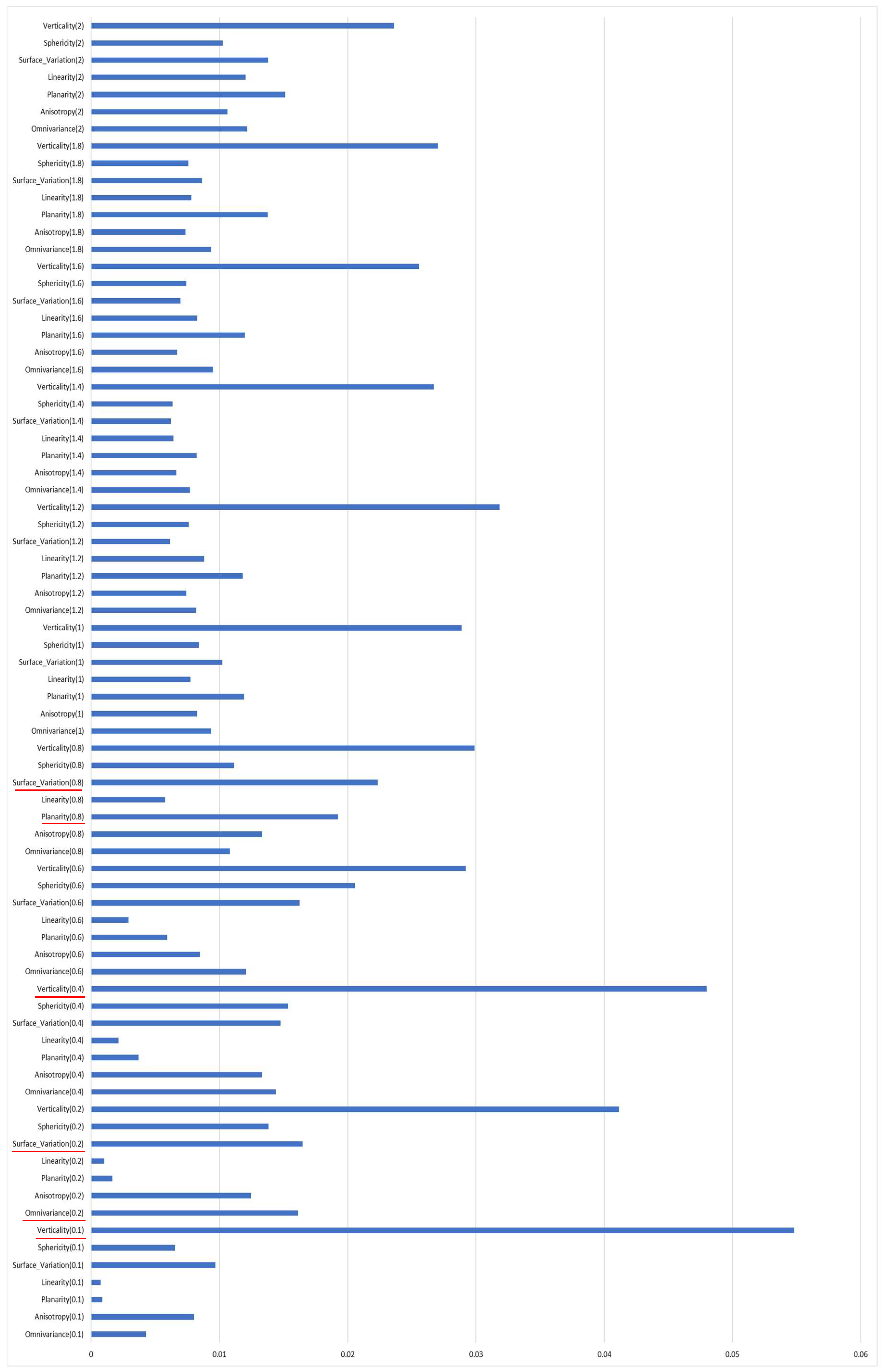
Therefore, to make the generalisation effective, it was essential to identify a small set of features able to perform similarly across different architectural datasets. For the analysis of the best features, we first considered the selection suggested by the RF algorithm, based on impurity reduction [42], starting from a multi-scale analysis done over the training set (Figure 6). Then, iteratively considering the most important features, only planarity P, omnivariance O, surface variation C, and verticality V, at specific radii (Table 2, Figure 7) were used. In addition, the absolute height was employed.
Once all the mentioned features had been extracted from all the datasets, we noticed that omnivariance O, and surface variation C, were presenting different ranges depending on the point cloud densities. Hence, we normalised them in the range 0–1 adopting the modified logistic function defined in [57], to facilitate the generalisation between the pre-trained model and the unseen scenarios.
3. Experiments and Results
3.1. Evaluation Method
Traditionally, the evaluation of a classification model is performed by splitting the labelled data into two sets, one used for training and the other one for testing. However, in this way, the evaluation procedure does not assess how the method generalises to a different framework.
In this paper, we first pre-trained a model over a limited portion (about 5M points) of a reference dataset (dataset A: Bologna–S. Stefano, Table 1), then we extended the classification to all the different datasets described in Table 1. In this way, we could evaluate the performances of the classifier at four different levels of generalisation:
- Changing city and acquisition technique: a modified version (model 2) of the pre-trained model 1 is tested on the TL dataset F (Table 7, Figure 12). Since the handheld scanning dataset was not provided with RGB values, a re-training round was necessary including exclusively height and geometry-based features.
Finally, for an exhaustive evaluation of each level, some portions of each classified dataset were taken into consideration and compared with the same manually annotated point clouds. The number of correct and incorrect predictions were summarised with count values and broken down by each class inside confusion matrices, that allows the visualisation of the performance of the algorithm (Table 3, Table 4, Table 5, Table 6 and Table 7). Each row of the matrix represents the instances in an actual class (ground truth), while each column represents the instances in a predicted class. From each confusion matrix we could then derive the following accuracy metrics:
● Precision: it is a ratio of the total detection by the classifier. It gives information about the model performance with respect to false positives (how many did we catch):
● Recall: it is a ratio of the correct detection over the total number of test samples and gives information about a classifier’s performance with respect to false negatives (how many did we miss):
● F1 score: it is used to compare the performance of the predictive model. It considers both the precision and recall values to compute the measures:
where = true positive (sum of the values in the diagonal position), = false positive (sum of the values in the column without the main diagonal one), = false negative (sum of the values in the row without the main diagonal one).
Precision, recall and the F1 score were first computed for each class using the above formula, then the arithmetic and weighted averages over all the classes were considered.
3.2. Results
From the observation of the accuracy metrics (Table 3, Table 4, Table 5, Table 6 and Table 7) and the results (Figure 8, Figure 9, Figure 10, Figure 11 and Figure 12), we can reasonably infer that both model 1 and model 2 were able to generalise over unseen datasets.
If we take into consideration Table 3, even if the training samples represent a portion of the tested dataset A, the results are still surprising (0.93 F1-score). In fact, these accuracy metrics have far exceeded our previous study results (0.80 F1-score) achieved over a smaller portion of the same Bologna dataset.
Concerning the second experiment (Table 4), the average of the arithmetic metrics is around 0.80. However, from a closer analysis, we can see that low values were achieved for the class other, which represents a small sample of the entire dataset. Hence, if we consider the weighted average, then the accuracy easily reaches 0.89. This kind of problem may be due to the lack of a representative annotation for this class within the training set. In particular, we can see that in dataset B and C some garbage cans (not present in dataset A) have been wrongly classified under facade or column (Figure 9c).
On the other hand, this problem was not present within experiments 3 and 4, where instead, the accuracy values were decreased because of some problem with the classes window and moulding, often confused with each other (Table 5 and Table 7). This is especially evident where the RGB values were not available in the point cloud (Table 7). A possible solution for this, in a future study, might be to include in the class window both glass and moulding.
The most problematic generalisation experiment was the one relative to dataset E, where the F1-score reached was only about 0.70 (Table 6). The peculiar type of windows and decorations of the medieval facades (Figure 11) has led to several classification problems. To solve these kinds of errors in future works, it might be useful to integrate the training set with the samples coming from this dataset.
Finally, quite satisfying results have been achieved testing the generalisation between datasets with different characteristics (Table 7).
The presented methodology and all the results are summarised in this video: https://www.youtube.com/watch?v=_68PdseUh3o.
Moreover, the Random Forest code we used, and the pre-trained classifier models are available at: https://github.com/3DOM-FBK/RF4PCC
4. Conclusions
This paper proved the capability of a pre-trained random forest (RF) model to generalise across different and unseen 3D heritage scenarios. Although a reduced number of datasets have been evaluated in this study, it is essential to consider that, except for the Trento Lodge case study, each dataset (streets or square) already contains a big differentiation of buildings within it.
The absence of a generalisation study using a standard machine learning approach in this field precludes a practical comparison between similar works. Nevertheless, if we would compare the average of our accuracy metrics with other results (e.g., [36] and [37]), we can say that at the moment our results reached better accuracy metrics, notwithstanding less training data and a faster prediction time.
The strengths of the presented approach can be summarised as follows:
- It is possible to classify a large dataset starting from a reduced number of annotated samples, saving time in both collecting and preparing data for training the algorithm; this is the first time that this has been demonstrated within the complex heritage field;
- The generalisation works even when training and test sets have different densities and the distribution of the points in the cloud is not uniform (Experiment 4, Figure 12);
- The quality of the results allows us to have a general idea of the distribution of the architectural classes and could support restoration works by providing approximate surface areas or volumes;
- The output can facilitate the scan-to-BIM problems, semantically separating elements in point clouds for the modelling procedure in a BIM environment;
- Automated classification methods can be used to accelerate the time-consuming process of the annotation of a significant number of datasets, in order to benchmark 3D heritages;
- The used RF model is easy to implement, and it does not require high computational efforts nor long learning or processing time.
On the other hand, we saw that when the test set does not follow the distribution of the training data, then the model does not perform as expected. Starting from this observation and considering previous research experiences [35,38], the authors believe that in the heritage field, particular case studies should be treated individually. However, it is possible, and it might be worth generating different pre-trained classifier models for macro-categories of architectures (e.g., classical architecture, Greek temples, gothic churches). In this view, we will consider in the future the possibility to generate simulated point clouds coming from BIM to further accelerate the annotation phase.
To conclude, the heritage domain is a sophisticated testfield for both machine and deep learning classification methods. For this reason, a new benchmark dataset [58] is going to be released in order to boost research activities in this field and become a central resource for the development of new, efficient and accurate methods for classifying heritage 3D data.
Author Contributions
Conceptualization, Eleonora Grilli; methodology, Eleonora Grilli; investigation, Eleonora Grilli and Fabio Remondino; resources, Fabio Remondino; data curation, Eleonora Grilli; writing—original draft preparation, Eleonora Grilli; writing—review and editing, Fabio Remondino; visualization, Eleonora Grilli; supervision, Fabio Remondino. All authors have read and agreed to the published version of the manuscript.
Funding
This research received external funding from the project “Artificial Intelligence for Cultural Heritage” (AI4CH), a joint Italy–Israel lab which was funded by the Italian Ministry of Foreign Affairs and International Cooperation (MAECI).
Conflicts of Interest
The authors declare no conflict of interest.
References
- Gruen, A. Reality-based generation of virtual environments for digital earth. Int. J. Digit. Earth 2008, 1, 88–106. [Google Scholar] [CrossRef]
- Remondino, F. Heritage Recording and 3D Modeling with Photogrammetry and 3D Scanning. Remote Sens. 2011, 3, 1104–1138. [Google Scholar] [CrossRef] [Green Version]
- Barsanti, S.G.; Remondino, F.; Fenández-Palacios, B.J.; Visintini, D. Critical Factors and Guidelines for 3D Surveying and Modelling in Cultural Heritage. Int. J. Herit. Digit. Era 2014, 3, 141–158. [Google Scholar] [CrossRef] [Green Version]
- Son, H.; Kim, C. Semantic as-built 3D modeling of structural elements of buildings based on local concavity and convexity. Adv. Eng. Inform. 2017, 34, 114–124. [Google Scholar] [CrossRef]
- Lu, Q.; Lee, S. Image-based technologies for constructing as-is building information models for existing buildings. J. Comput. Civ. Eng. 2017, 31, 04017005. [Google Scholar] [CrossRef]
- Rebolj, D.; Pučko, Z.; Babič, N.; Bizjak, M.; Mongus, D. Point cloud quality requirements for Scan-vs-BIM based automated construction progress monitoring. Autom. Constr. 2017, 84, 323–334. [Google Scholar] [CrossRef]
- Bassier, M.; Yousefzadeh, M. Comparison of 2D and 3D wall reconstruction algorithms from point cloud data for as-built BIM. J. Inf. Technol. Constr. 2020, 25, 173–192. [Google Scholar] [CrossRef]
- Apollonio, F.I.; Basilissi, V.; Callieri, M.; Dellepiane, M.; Gaiani, M.; Ponchio, F.; Rizzo, F.; Rubino, A.R.; Scopigno, R.; Sobra’, G. A 3D-centered information system for the documentation of a complex restoration intervention. J. Cult. Herit. 2018, 29, 89–99. [Google Scholar] [CrossRef]
- Valero, E.; Bosché, F.; Forster, A. Automatic segmentation of 3D point clouds of rubble masonry walls, and its application to building surveying, repair and maintenance. Autom. Constr. 2018, 96, 29–39. [Google Scholar] [CrossRef]
- Sánchez-Aparicio, L.; Del Pozo, S.; Ramos, L.; Arce, A.; Fernandes, F. Heritage site preservation with combined radiometric and geometric analysis of TLS data. Autom. Constr. 2018, 24–39. [Google Scholar] [CrossRef]
- Roussel, R.; Bagnéris, M.; De Luca, L. A digital diagnosis for the «Autumn» statue (Marseille, France): Photogrammetry, digital cartography and construction of a thesaurus. ISPRS Int. Arch. Photogramm. Remote Sens. Spat. Inf. Sci. 2019, XLII-2/W15, 1039–1046. [Google Scholar] [CrossRef] [Green Version]
- Bosché, F. Automated recognition of 3D CAD model objects in laser scans and calculation of as-built dimensions for dimensional compliance control in construction. Adv. Eng. informatics 2010, 24, 107–118. [Google Scholar] [CrossRef]
- Ordóñez, C.; Martínez, J.; Arias, P.; Armesto, J. Measuring building façades with a low-cost close-range photogrammetry system. Autom. Constr. 2010, 19, 742–749. [Google Scholar] [CrossRef]
- Mizoguchi, T.; Koda, Y.; Iwaki, I.; Wakabayashi, H.; Kobayashi, Y.S.K.; Hara, Y.; Lee, H. Quantitative scaling evaluation of concrete structures based on terrestrial laser scanning. Autom. Constr. 2013, 35, 263–274. [Google Scholar] [CrossRef]
- Kashani, A.; Graettinger, A. Cluster-based roof covering damage detection in ground-based lidar data. Autom. Constr. 2015, 58, 19–27. [Google Scholar] [CrossRef]
- Barazzetti, L.; Banfi, F.; Brumana, R.; Gusmeroli, G.; Previtali, M.; Schiantarelli, G. Cloud-to-BIM-to-FEM: Structural simulation with accurate historic BIM from laser scans. Simul. Model. Pract. Theory 2015, 57, 71–87. [Google Scholar] [CrossRef]
- Banfi, F. BIM orientation: Grades of generation and information for different type of analysis and management process. Int. Arch. Photogramm. Remote Sens. Spat. Inf. Sci. 2017, XLII–2/W5, 57–64. [Google Scholar] [CrossRef] [Green Version]
- Bitelli, G.; Castellazzi, G.; D’Altri, A.; De Miranda, S.; Lambertini, A.; Selvaggi, I. Automated voxel model from point clouds for structural analysis of cultural heritage ISPRS-Int. Int. Arch. Photogramm. Remote Sens. Spat. Inf. Sci. 2016, 41, 191–197. [Google Scholar] [CrossRef]
- Grilli, E.; Menna, F.; Remondino, F. A review of point cloud segmentation and classification algorithms. ISPRS Int. Arch. Photogramm. Remote Sens. Spat. Inf. Sci. 2017, XLII-2/W3, 339–344. [Google Scholar] [CrossRef] [Green Version]
- Vosselman, G. Point cloud segmentation for urban scene classification. ISPRS Int. Arch. Photogramm. Remote Sens. Spat. Inf. Sci. 2013, XL-7/W2, 257–262. [Google Scholar] [CrossRef] [Green Version]
- Weinmann, M.; Jutzi, B.; Mallet, C. Feature relevance assessment for the semantic interpretation of 3D point cloud data. ISPRS Ann. Photogramm. Remote Sens. Spat. Inf. Sci. 2013, II-5/W2, 313–318. [Google Scholar] [CrossRef] [Green Version]
- Niemeyer, J.; Rottensteiner, F.; Soergel, U. Contextual classification of lidar data and building object detection in urban areas. ISPRS J. Photogramm. Remote Sens. 2014, 87, 152–165. [Google Scholar] [CrossRef]
- Charles, R.Q.; Su, H.; Kaichun, M.; Guibas, L.J. PointNet: Deep Learning on Point Sets for 3D Classification and Segmentation. In Proceedings of the Conference on Computer Vision and Pattern Recognition (CVPR), Honolulu, HI, USA, 21–26 July 2017; pp. 77–85. [Google Scholar]
- Qi, C.R.; Yi, L.; Su, H.; Guibas, L.J. PointNet++: Deep Hierarchical Feature Learning on Point Sets in a Metric Space. In Proceedings of the Conference on Neural Information Processing Systems (NIPS), Long Beach, CA, USA, 24 January 2019. [Google Scholar]
- Dargan, S.; Kumar, M.; Ayyagari, M.R.; Kumar, G. A survey of Deep Learning and its applications: A new paradigm to Machine Learning. Arch. Comput. Methods Eng. 2019, 26, 1–22. [Google Scholar] [CrossRef]
- Griffiths, D.; Boehm, J. A Review on Deep Learning Techniques for 3D Sensed Data Classification. Remote Sens. 2019, 11, 1499. [Google Scholar] [CrossRef] [Green Version]
- O’Mahony, N.; Campbell, S.; Carvalho, A.; Harapanahalli, S.; Hernandez, G.V.; Krpalkova, L.; Riordan, D.; Walsh, J. Deep Learning vs. Traditional Computer Vision. arXiv 2019, arXiv:1910.13796. [Google Scholar]
- Chang, A.X.; Funkhouser, T.; Guibas, L.; Hanrahan, P.; Huang, Q.; Li, Z.; Savarese, S.; Savva, M.; Song, S.; Su, H.; et al. Shapenet: An information-rich 3d model repository. arXiv 2015, arXiv:1512.03012v1. [Google Scholar]
- Armeni, I.; Sener, O.; Zamir, A.R.; Savarese, S. Joint 2D-3D-Semantic Data for Indoor Scene Understanding. arXiv 2017, arXiv:1702.01105. [Google Scholar]
- Dai, A.; Chang, A.X.; Savva, M.; Halber, M.; Funkhouser, T.; Nießner, M. ScanNet: Richly-annotated 3D Reconstructions of Indoor Scenes. In Proceedings of the IEEE Conference on Computer Vision and Pattern Recognition, Honolulu, HI, USA, 21–26 July 2017; pp. 5828–5839. [Google Scholar]
- Munoz, D.; Bagnell, J.A.; Vandapel, N.; Hebert, M. Contextual classification with functional max-margin markov networks. In Proceedings of the 2009 IEEE Conference on Computer Vision and Pattern Recognition, Miami, FL, USA, 20–26 June 2009; pp. 975–982. [Google Scholar]
- Serna, A.; Marcotegui, B.; Goulette, F.; Deschaud, J.-E. Paris-rue-Madame database: A 3D mobile laser scanner dataset for benchmarking urban detection, segmentation and classification methods. In Proceedings of the 3rd International Conference on Pattern Recognition, Applications and Methods ICPRAM, Angers, Loire Valley, France, 6–8 March 2014. [Google Scholar]
- Cordts, M.; Omran, M.; Ramos, S.; Rehfeld, T.; Enzweiler, M.; Benenson, R.; Franke, U.; Roth, S.; Schiele, B.; R&d, D.A.; et al. The Cityscapes Dataset for Semantic Urban Scene Understanding. In Proceedings of the IEEE Conference on Computer Vision and Pattern Recognition, Las Vegas, NV, USA, 26 June–1 July 2016. [Google Scholar]
- Hackel, T.; Savinov, N.; Ladicky, L.; Wegner, J.D.; Schindler, K.; Pollefeys, M. Semantic3D.net: A new Large-scale Point Cloud Classification Benchmark. arXiv 2017, arXiv:1704.03847. [Google Scholar] [CrossRef] [Green Version]
- Grilli, E.; Remondino, F. Classification of 3D Digital Heritage. Remote Sens. 2019, 11, 847. [Google Scholar] [CrossRef] [Green Version]
- Murtiyoso, A.; Grussenmeyer, P. Virtual Disassembling of Historical Edifices: Experiments and Assessments of an Automatic Approach for Classifying Multi-Scalar Point Clouds into Architectural Elements. Sensors 2020, 20, 2161. [Google Scholar] [CrossRef] [Green Version]
- Pierdicca, R.; Paolanti, M.; Matrone, F.; Martini, M.; Morbidoni, C.; Malinverni, E.S.; Frontoni, E.; Lingua, A.M. Point Cloud Semantic Segmentation Using a Deep Learning Framework for Cultural Heritage. Remote Sens. 2020, 12, 1005. [Google Scholar] [CrossRef] [Green Version]
- Grilli, E.; Farella, E.M.; Torresani, A.; Remondino, F. Geometric features analysis for the classification of cultural heritage point clouds. ISPRS Int. Arch. Photogramm. Remote Sens. Spat. Inf. Sci. 2019, XLII-2/W15, 541–548. [Google Scholar] [CrossRef] [Green Version]
- Weiss, K.; Khoshgoftaar, T.M.; Wang, D.D. A survey of transfer learning. J. Big Data 2016, 3, 9. [Google Scholar] [CrossRef] [Green Version]
- Sarkar, D.; Bali, R.; Ghosh, T. Hands-On Transfer Learning with Python: Implement Advanced Deep Learning and Neural Network Models Using TensorFlow and Keras; Packt Publishing Ltd.: Birmingham, UK, 2018. [Google Scholar]
- Remondino, F.; Gaiani, M.; Apollonio, F.; Ballabeni, A.; Ballabeni, M.; Morabito, D. 3D documentation of 40 km of historical porticoes—The challenge. Int. Arch. Photogramm. Remote Sens. Spat. Inf. Sci. 2016, 41, 711–718. [Google Scholar] [CrossRef]
- Breiman, L. Random Forests. Mach. Learn. 2001, 45, 5–32. [Google Scholar] [CrossRef] [Green Version]
- Bassier, M.; Genechten, B.V.; Vergauwen, M. Classification of sensor independent point cloud data of building objects using random forests. J. Build. Eng. 2019, 21, 468–477. [Google Scholar] [CrossRef]
- Kogut, T.; Weistock, M. Classifying airborne bathymetry data using the Random Forest algorithm. Remote Sens. Lett. 2019, 10, 874–882. [Google Scholar] [CrossRef]
- Poux, F.; Billen, R. Geo-Information Voxel-based 3D Point Cloud Semantic Segmentation: Unsupervised Geometric and Relationship Featuring vs Deep Learning Methods. ISPRS Int. J. Geo-Inf. 2019, 8, 213. [Google Scholar] [CrossRef] [Green Version]
- Grilli, E.; Ozdemir, E.; Remondino, F. Application of machine and deep learning strategies for the classification of heritage point clouds. Int. Arch. Photogramm. Remote Sens. Spat. Inf. Sci. 2019, XLII-4/W18, 447–454. [Google Scholar] [CrossRef] [Green Version]
- Pedregosa, F.; Varoquaux, G.; Gramfort, A.; Michel, V.; Thirion, B.; Grisel, O.; Blondel, M.; Prettenhofer, P.; Weiss, R.; Dubourg, V.; et al. Scikit-learn: Machine Learning in Python. J. Mach. Learn. Res. 2011, 12, 2825–2830. [Google Scholar]
- Malinverni, E.S.; Pierdicca, R.; Paolanti, M.; Martini, M.; Morbidoni, C.; Matrone, F.; Lingua, A. Deep learning for semantic segmentation of 3D point cloud. ISPRS Int. Arch. Photogramm. Remote Sens. Spat. Inf. Sci. 2019, XLII-2/W15, 735–742. [Google Scholar] [CrossRef] [Green Version]
- Semantic Segmentation Editor. Available online: https://github.com/GerasymenkoS/semantic-segmentation-editor (accessed on 27 April 2020).
- Jurio, A.; Pagola, M.; Galar, M.; Lopez-Molina, C.; Paternain, D. A comparison study of different color spaces in clustering based image segmentation. In International Conference on Information Processing and Management of Uncertainty in Knowledge-Based Systems; Springer: Berlin/Heidelberg, Germany, 2010; pp. 532–541. [Google Scholar]
- Chehata, N.; Guo, L.; Mallet, C. Airborne lidar feature selection for urban classification using random forests. Laser Scanning IAPRS 2009, XXXVIII, 207–212. [Google Scholar]
- Weinmann, M.; Jutzi, B.; Mallet, C.; Weinmann, M. Geometric features and their relevance for 3D point cloud classification. ISPRS Ann. Photogramm. Remote Sens. Spat. Inf. Sci. 2017, IV-1/W1, 157–164. [Google Scholar] [CrossRef] [Green Version]
- Hackel, T.; Wegner, J.D.; Schindler, K. Fast Semantic Segmentation of 3D Point Clouds with Strongly Varying Density. ISPRS Ann. Photogramm. Remote Sens. Spat. Inf. Sci 2016, III–3, 177–184. [Google Scholar] [CrossRef]
- Blomley, R.; Weinmann, M.; Leitloff, J.; Jutzi, B. Shape distribution features for point cloud analysis-a geometric histogram approach on multiple scales. ISPRS Ann. Photogramm. Remote Sens. Spat. Inf. Sci. 2014, 2, 9–16. [Google Scholar] [CrossRef] [Green Version]
- Weinmann, M.; Schmidt, A.; Mallet, C.; Hinz, S.; Rottensteiner, F.; Jutzi, B. Contextual classification of point cloud data by exploiting individual 3D neigbourhoods. ISPRS Ann. Photogramm. Remote Sens. Spat. Inf. Sci. 2015, II-3/W4, 271–278. [Google Scholar] [CrossRef] [Green Version]
- Thomas, H.; Deschaud, J.-E.; Marcotegui, B.; Goulette, F.; Le Gall, Y. Semantic Classification of 3D Point Clouds with Multiscale Spherical Neighborhoods. In Proceedings of the International Conference on 3D Vision (3DV), Verona, Italy, 5–8 September 2018; pp. 390–398. [Google Scholar]
- Mauro, M.; Riemenschneider, H.; Signoroni, A.; Leonardi, R.; van Gool, L. A unified framework for content-aware view selection and planning through view importance. In Proceedings of the British Machine Vision Conference BMVC 2014, Nottingham, UK, 1–5 September 2014; pp. 1–11. [Google Scholar]
- Matrone, F.; Lingua, A.; Pierdicca, R.; Malinverni, E.S.; Paolanti, M.; Grilli, E.; Remondino, F.; Murtiyoso, A.; Landes, T. A benchmark for large-scale heritage point cloud semantic segmentation. ISPRS Int. Arch. Photogramm. Remote Sens. Spat. Inf. Sci. 2020, XLIII-B2, 4558–4567. [Google Scholar]
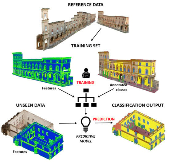
Figure 1.
Three-dimensional (3D) point cloud classification process where a portion of the dataset is used as training set.
Figure 1.
Three-dimensional (3D) point cloud classification process where a portion of the dataset is used as training set.

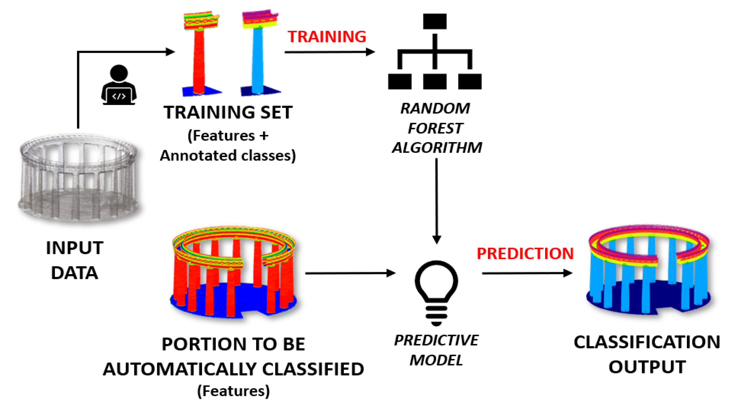
Figure 2.
Three-dimensional (3D) point cloud classification process for unseen datasets. Some portions are extracted from the reference point cloud, manually annotated and enriched with selected features (Section 2.2). A random forest algorithm is then trained to generate a predictive model. This model is used to classify unseen scenarios.

Figure 3.
A closer view of the reference dataset, where it is possible to see the big variety of the architectural elements (facades, windows, arches, doors, columns, etc.).
Figure 3.
A closer view of the reference dataset, where it is possible to see the big variety of the architectural elements (facades, windows, arches, doors, columns, etc.).

Figure 4.
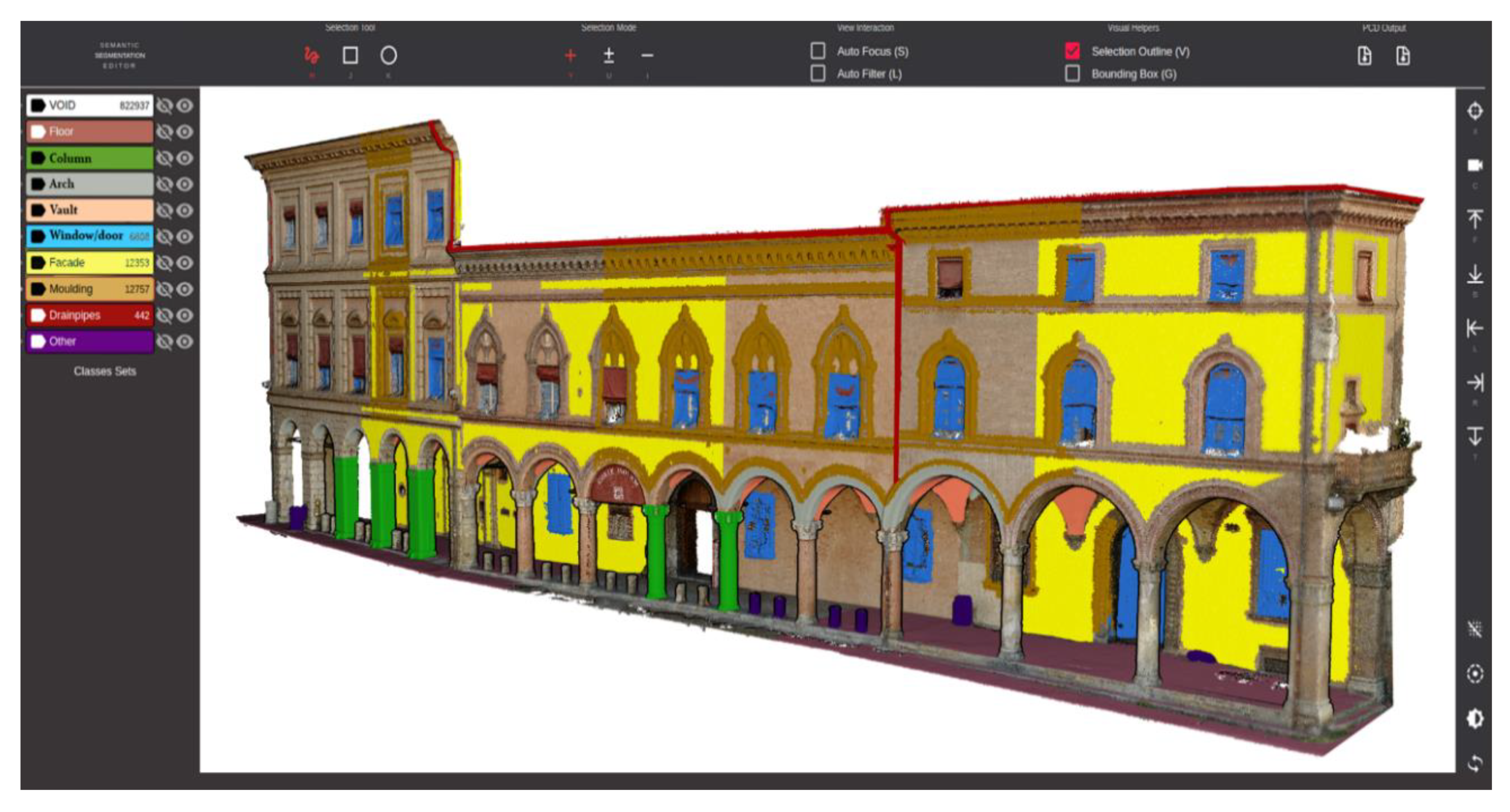
Our in-house web-based annotation tool.

Figure 5.
Use of the colour component b* to facilitate the distinction between the windows and walls.
Figure 5.
Use of the colour component b* to facilitate the distinction between the windows and walls.

Figure 6.
Feature importance ranking for a multi-scale classification. The features used in this study have been underlined in red.
Figure 6.
Feature importance ranking for a multi-scale classification. The features used in this study have been underlined in red.

Figure 7.
Example of the geometric features used for the classification procedure on Table 1 datasets: (a) planarity: it can facilitate the identification of arches and columns; (b) omnivariance and (c) surface variation: they highlight the discontinuities between the walls, mouldings and the windows; (d) verticality: it is essential to distinguish floors from facades.

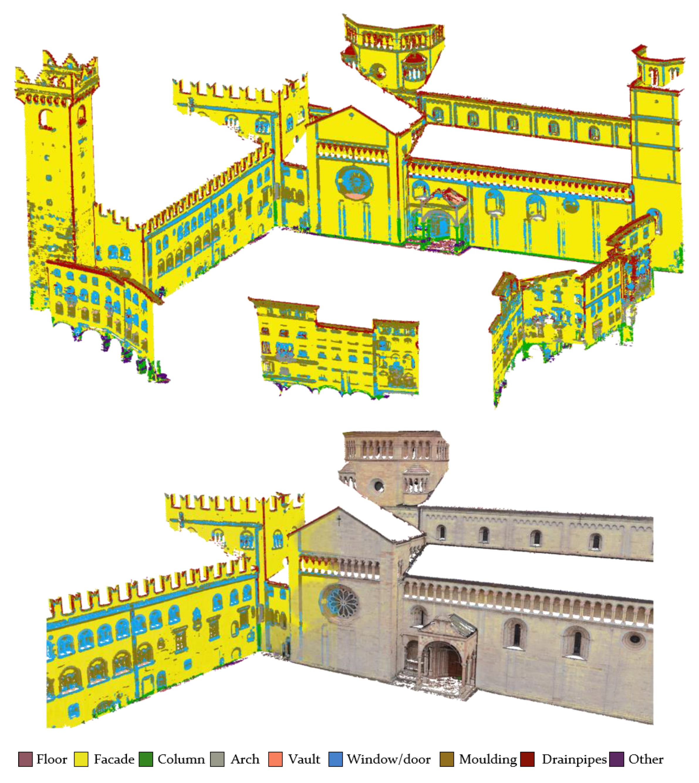
Figure 8.
Classification results: generalisation level #1, within dataset A.

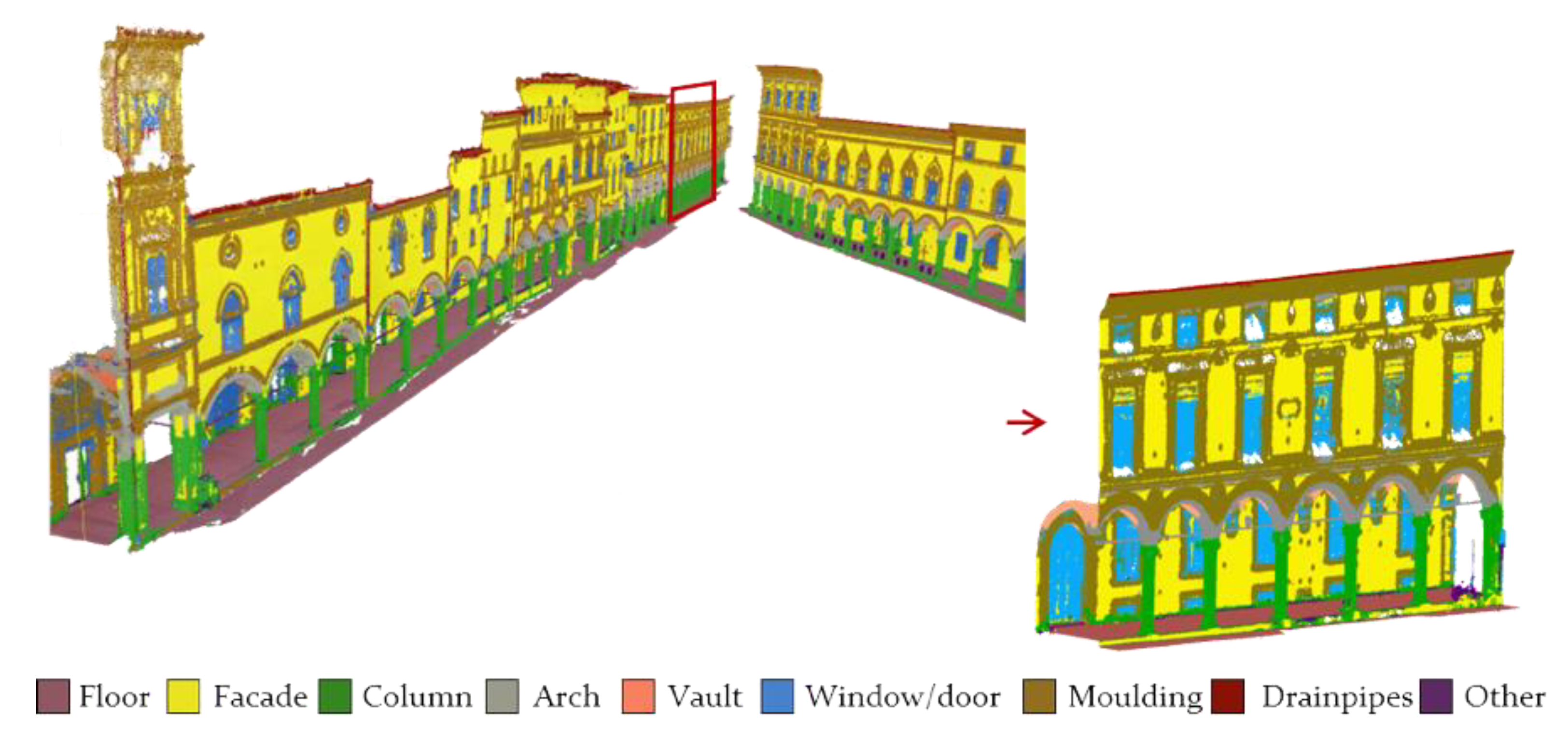
Figure 9.
Classification results: generalisation level #2: (a) dataset B, (b) dataset C, (c) a comparison between the prediction and the ground truth shows the classification errors within the class other.
Figure 9.
Classification results: generalisation level #2: (a) dataset B, (b) dataset C, (c) a comparison between the prediction and the ground truth shows the classification errors within the class other.

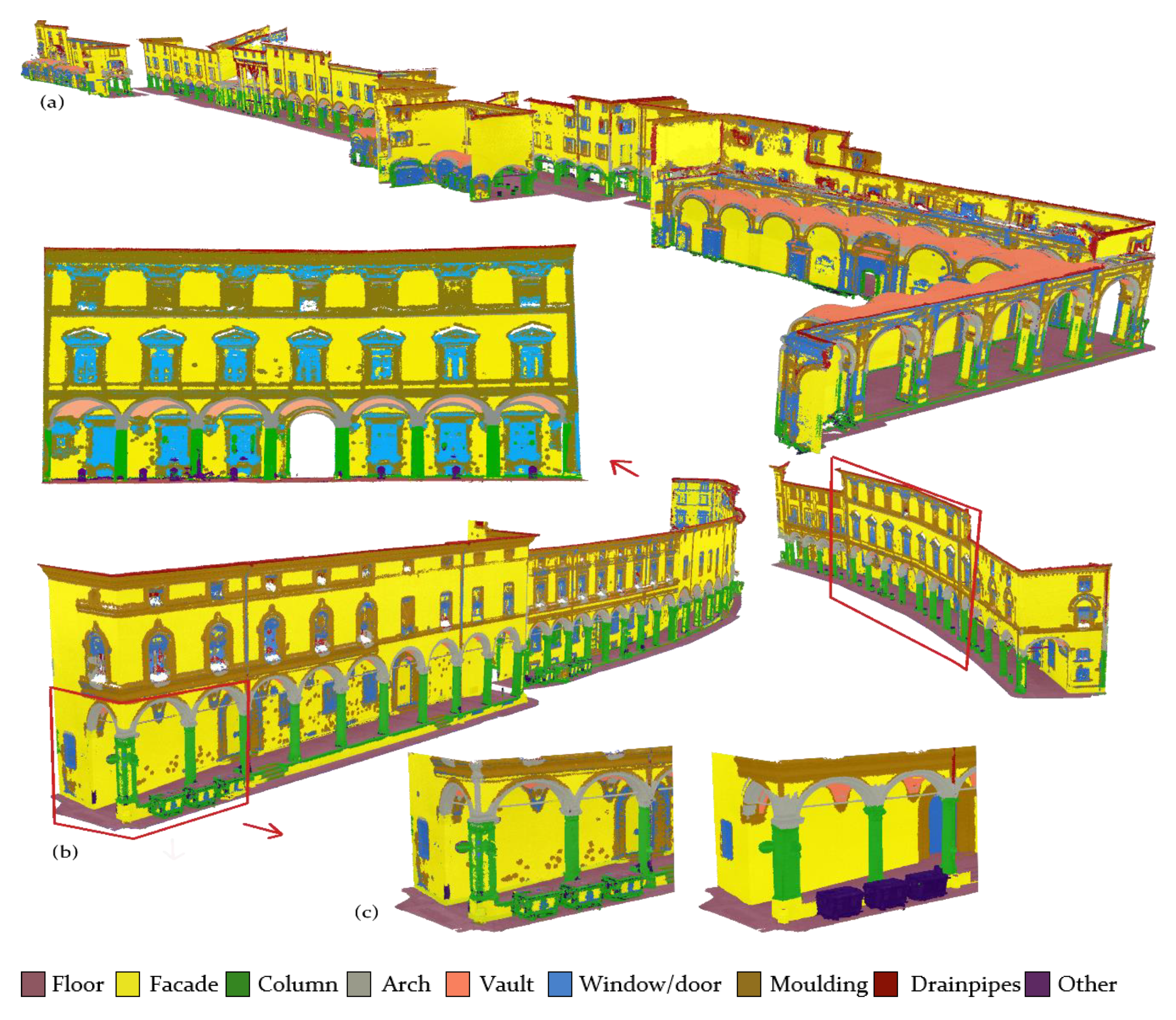
Figure 10.
Classification results: generalisation level #3, dataset D.

Figure 11.
Classification results: generalisation level #3, dataset E. A closer view shows how this architectural style is different from the one in the training dataset (Figure 4).
Figure 11.
Classification results: generalisation level #3, dataset E. A closer view shows how this architectural style is different from the one in the training dataset (Figure 4).

Figure 12.
Classification results: generalisation level #4, dataset F. Please note that despite the decreasing spatial resolution from ground to top, the generalisation could work.
Figure 12.
Classification results: generalisation level #4, dataset F. Please note that despite the decreasing spatial resolution from ground to top, the generalisation could work.


Table 1.
Datasets considered in the presented work to validate the pre-trained model and the generalisation method (Av. D. = average distance between points, L= length of the facades).
Table 1.
Datasets considered in the presented work to validate the pre-trained model and the generalisation method (Av. D. = average distance between points, L= length of the facades).
| DATASET | ACQUISITION | POINTS (M) | AV. D. (cm) | L (m) | ||
|---|---|---|---|---|---|---|
| A | Bologna– S. Stefano |  | Photogrammetry | 14 | 0.8 | 230 |
| B | Bologna– S. Maggiore |  | Photogrammetry | 22 | 0.8 | 330 |
| C | Bologna–Castiglione |  | Photogrammetry | 14 | 0.8 | 235 |
| D | Trento–Lodge |  | Photogrammetry | 6 | 1.0 | 100 |
| E | Trento–Square |  | Photogrammetry | 11 | 1.3 | 330 |
| F | Trento–Streets |  | Handheld scanning | 13 | From 0.2 to 15.0 | 810 |
Table 2.
Geometric features considered to train the model with their relative neighbourhood size.
| FEATURE | FORMULA | NEIGHBOURHOOD SIZE (m) |
|---|---|---|
| Planarity | Equation (1) | 0.8 |
| Omnivariance | Equation (2) | 0.2 |
| Surface variation | Equation (3) | 0.2, 0.8 |
| Verticality | Equation (4) | 0.1, 0.4 |
Table 3.
Evaluation metrics: generalisation level #1, within dataset A.
| CLASS | Floor | Facade | Column | Arch | Vault | Window | Moulding | Drainpipe | Other | Precision | Recall | F1-Score |
|---|---|---|---|---|---|---|---|---|---|---|---|---|
| floor | 546304 | 1 | 0 | 0 | 0 | 0 | 0 | 0 | 2619 | 1.00 | 1.00 | 1.00 |
| facade | 0 | 361751 | 4763 | 1175 | 0 | 185 | 0 | 0 | 2 | 0.98 | 0.99 | 0.99 |
| column | 0 | 218 | 59772 | 326 | 0 | 0 | 0 | 0 | 632 | 0.98 | 0.92 | 0.95 |
| arch | 0 | 507 | 94 | 57632 | 3972 | 20 | 5363 | 0 | 0 | 0.85 | 0.92 | 0.89 |
| vault | 0 | 0 | 0 | 3201 | 629809 | 1221 | 243 | 0 | 0 | 0.99 | 0.99 | 0.99 |
| window | 0 | 3030 | 0 | 2 | 24 | 78565 | 10531 | 852 | 0 | 0.84 | 0.88 | 0.86 |
| moulding | 0 | 200 | 143 | 227 | 1107 | 8668 | 304610 | 512 | 0 | 0.97 | 0.95 | 0.96 |
| drainpipe | 0 | 2 | 7 | 23 | 2 | 617 | 23 | 5641 | 0 | 0.89 | 0.81 | 0.85 |
| other | 111 | 137 | 230 | 0 | 0 | 0 | 0 | 0 | 18071 | 0.97 | 0.85 | 0.91 |
| ARITHMETIC AVERAGE | 0.94 | 0.92 | 0.93 | |||||||||
| WEIGHTED AVERAGE | 0.98 | 0.98 | 0.98 | |||||||||
Table 4.
Evaluation metrics: generalisation level #2, B–C datasets. The most critical F1 values are reported in italics (other class).
Table 4.
Evaluation metrics: generalisation level #2, B–C datasets. The most critical F1 values are reported in italics (other class).
| CLASS | Floor | Facade | Column | Arch | Vault | Window | Moulding | Drainpipe | Other | Precision | Recall | F1-Score |
|---|---|---|---|---|---|---|---|---|---|---|---|---|
| floor | 890967 | 207 | 20 | 0 | 0 | 4 | 0 | 0 | 3850 | 1.00 | 0.94 | 0.97 |
| facade | 3704 | 1084815 | 2530 | 16981 | 701 | 36776 | 17439 | 2 | 24741 | 0.91 | 0.91 | 0.91 |
| column | 20888 | 39614 | 200758 | 2672 | 0 | 961 | 1483 | 7 | 4664 | 0.74 | 0.85 | 0.79 |
| arch | 0 | 6855 | 21979 | 217040 | 6484 | 4477 | 16238 | 73 | 0 | 0.79 | 0.78 | 0.79 |
| vault | 76 | 0 | 0 | 27526 | 862579 | 833 | 1174 | 17 | 1 | 0.97 | 0.98 | 0.97 |
| window | 892 | 7801 | 163 | 657 | 4214 | 185498 | 51981 | 3231 | 677 | 0.73 | 0.66 | 0.69 |
| moulding | 4736 | 48394 | 13 | 14625 | 9687 | 44061 | 660871 | 815 | 74 | 0.84 | 0.88 | 0.86 |
| drainpipe | 0 | 9 | 17 | 26 | 0 | 8149 | 2478 | 25715 | 0 | 0.71 | 0.86 | 0.78 |
| other | 26107 | 5801 | 10828 | 0 | 5 | 519 | 385 | 0 | 34275 | 0.44 | 0.50 | 0.47 |
| ARITHMETIC AVERAGE | 0.79 | 0.82 | 0.80 | |||||||||
| WEIGHTED AVERAGE | 0.89 | 0.89 | 0.89 | |||||||||
Table 5.
Evaluation metrics: generalisation level #3, dataset D. The most critical F1 values are reported in italics (window and moulding classes).
Table 5.
Evaluation metrics: generalisation level #3, dataset D. The most critical F1 values are reported in italics (window and moulding classes).
| CLASS | Floor | Facade | Column | Arch | Vault | Window | Moulding | Drainpipe | Other | Precision | Recall | F1-Score |
|---|---|---|---|---|---|---|---|---|---|---|---|---|
| floor | 100514 | 613 | 787 | 0 | 0 | 0 | 184 | 0 | 3388 | 0.95 | 0.99 | 0.97 |
| facade | 0 | 204720 | 1305 | 341 | 0 | 4587 | 25349 | 0 | 71 | 0.87 | 0.94 | 0.90 |
| column | 39 | 3614 | 47864 | 1748 | 0 | 638 | 1073 | 0 | 877 | 0.86 | 0.84 | 0.85 |
| arch | 0 | 81 | 2923 | 20101 | 1665 | 242 | 992 | 0 | 0 | 0.77 | 0.79 | 0.78 |
| vault | 0 | 0 | 22 | 396 | 44387 | 450 | 533 | 0 | 0 | 0.97 | 0.95 | 0.96 |
| window | 19 | 5154 | 164 | 389 | 516 | 20424 | 13188 | 27 | 72 | 0.51 | 0.49 | 0.50 |
| moulding | 8 | 3203 | 1534 | 2376 | 328 | 15273 | 74301 | 1319 | 634 | 0.75 | 0.64 | 0.69 |
| drainpipe | 0 | 0 | 0 | 0 | 0 | 0 | 685 | 3047 | 11 | 0.81 | 0.69 | 0.75 |
| other | 832 | 143 | 2344 | 0 | 0 | 16 | 17 | 0 | 21208 | 0.86 | 0.81 | 0.83 |
| ARITHMETIC AVERAGE | 0.82 | 0.79 | 0.80 | |||||||||
| WEIGHTED AVERAGE | 0.84 | 0.85 | 0.85 | |||||||||
Table 6.
Evaluation metrics: generalisation level #3, dataset E. The most critical F1 values are reported in italics.
Table 6.
Evaluation metrics: generalisation level #3, dataset E. The most critical F1 values are reported in italics.
| CLASS | Floor | Facade | Column | Arch | Vault | Window | Moulding | Drainpipe | Other | Precision | Recall | F1-Score |
|---|---|---|---|---|---|---|---|---|---|---|---|---|
| floor | 8328 | 46 | 311 | 0 | 0 | 0 | 0 | 0 | 2253 | 0.76 | 0.97 | 0.85 |
| facade | 0 | 338699 | 3667 | 11911 | 1519 | 19313 | 6277 | 806 | 599 | 0.88 | 0.98 | 0.93 |
| column | 0 | 2286 | 40760 | 80 | 0 | 395 | 0 | 0 | 5831 | 0.83 | 0.56 | 0.66 |
| arch | 0 | 933 | 3494 | 63599 | 137 | 90 | 49 | 192 | 2966 | 0.89 | 0.70 | 0.78 |
| vault | 0 | 0 | 0 | 0 | 10924 | 0 | 6377 | 0 | 0 | 0.63 | 0.45 | 0.53 |
| window | 0 | 373 | 9432 | 8012 | 4913 | 118873 | 20431 | 1784 | 0 | 0.73 | 0.61 | 0.66 |
| moulding | 0 | 438 | 18 | 6716 | 6576 | 51118 | 160958 | 38202 | 291 | 0.61 | 0.82 | 0.70 |
| drainpipe | 0 | 1194 | 0 | 260 | 0 | 1279 | 3196 | 34627 | 0 | 0.85 | 0.46 | 0.60 |
| other | 251 | 2991 | 15559 | 0 | 15 | 3399 | 3 | 0 | 27772 | 0.56 | 0.70 | 0.62 |
| ARITHMETIC AVERAGE | 0.75 | 0.69 | 0.70 | |||||||||
| WEIGHTED AVERAGE | 0.77 | 0.80 | 0.78 | |||||||||
Table 7.
Evaluation metrics: generalisation level #4, dataset F. The most critical F1 values are reported in italics (window and moulding classes).
Table 7.
Evaluation metrics: generalisation level #4, dataset F. The most critical F1 values are reported in italics (window and moulding classes).
| CLASS | Floor | Facade | Column | Arch | Vault | Window | Moulding | Drainpipe | Other | Precision | Recall | F1-Score |
|---|---|---|---|---|---|---|---|---|---|---|---|---|
| floor | 2010296 | 0 | 78 | 0 | 0 | 38 | 16 | 0 | 1664 | 1.00 | 1.00 | 1.00 |
| facade | 1226 | 409440 | 7228 | 162 | 0 | 10308 | 6406 | 0 | 286 | 0.94 | 0.87 | 0.90 |
| column | 1574 | 2610 | 95728 | 5846 | 44 | 328 | 3068 | 0 | 4688 | 0.84 | 0.86 | 0.85 |
| arch | 0 | 682 | 3496 | 40202 | 792 | 778 | 4752 | 0 | 0 | 0.79 | 0.77 | 0.78 |
| vault | 0 | 0 | 0 | 3330 | 88774 | 1032 | 656 | 0 | 0 | 0.95 | 0.97 | 0.96 |
| window | 0 | 9174 | 1276 | 484 | 900 | 40848 | 30546 | 0 | 32 | 0.49 | 0.51 | 0.50 |
| moulding | 368 | 50698 | 2146 | 1984 | 1066 | 26376 | 148602 | 1370 | 34 | 0.64 | 0.75 | 0.69 |
| drainpipe | 0 | 0 | 0 | 0 | 0 | 54 | 2638 | 6094 | 0 | 0.69 | 0.81 | 0.75 |
| other | 6776 | 142 | 1754 | 0 | 0 | 144 | 1268 | 22 | 42416 | 0.81 | 0.86 | 0.83 |
| ARITHMETIC AVERAGE | 0.79 | 0.82 | 0.81 | |||||||||
| WEIGHTED AVERAGE | 0.94 | 0.93 | 0.93 | |||||||||
© 2020 by the authors. Licensee MDPI, Basel, Switzerland. This article is an open access article distributed under the terms and conditions of the Creative Commons Attribution (CC BY) license (http://creativecommons.org/licenses/by/4.0/).
Share and Cite
MDPI and ACS Style
Grilli, E.; Remondino, F. Machine Learning Generalisation across Different 3D Architectural Heritage. ISPRS Int. J. Geo-Inf. 2020, 9, 379. https://0-doi-org.brum.beds.ac.uk/10.3390/ijgi9060379
AMA Style
Grilli E, Remondino F. Machine Learning Generalisation across Different 3D Architectural Heritage. ISPRS International Journal of Geo-Information. 2020; 9(6):379. https://0-doi-org.brum.beds.ac.uk/10.3390/ijgi9060379
Chicago/Turabian StyleGrilli, Eleonora, and Fabio Remondino. 2020. "Machine Learning Generalisation across Different 3D Architectural Heritage" ISPRS International Journal of Geo-Information 9, no. 6: 379. https://0-doi-org.brum.beds.ac.uk/10.3390/ijgi9060379
Note that from the first issue of 2016, this journal uses article numbers instead of page numbers. See further details here.