Spatiotemporal Patterns and Driving Factors on Crime Changing During Black Lives Matter Protests

 , , ,
, , ,
Abstract
:1. Introduction
2. Materials and Methods
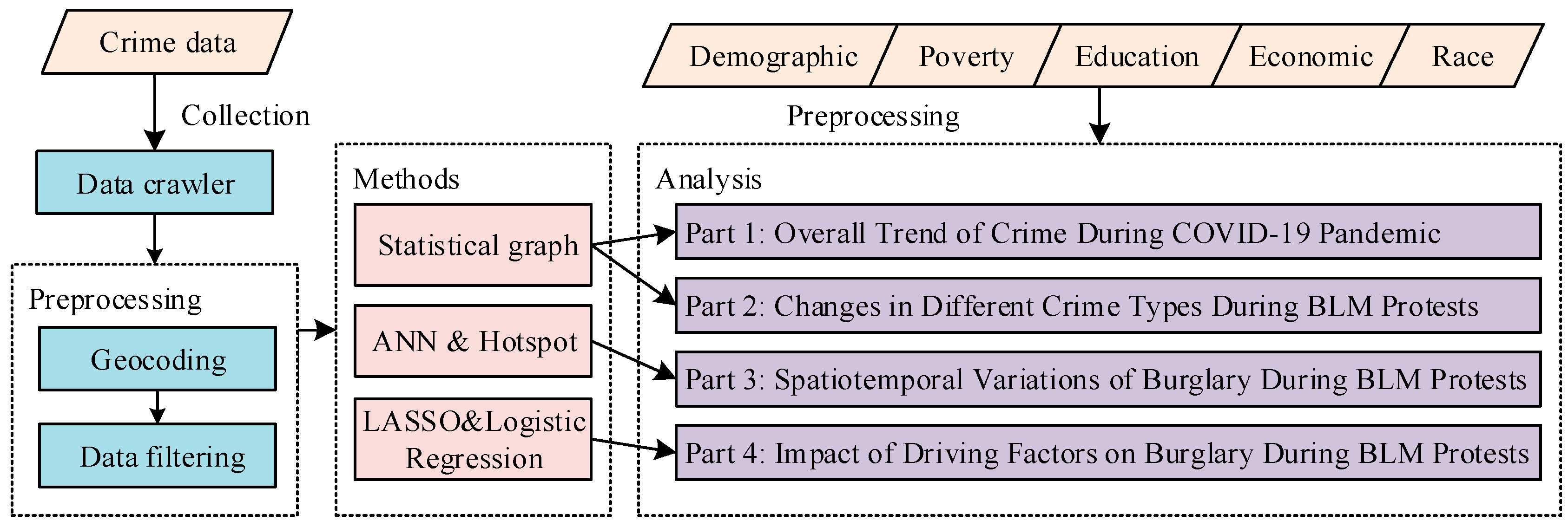
2.1. Workflow
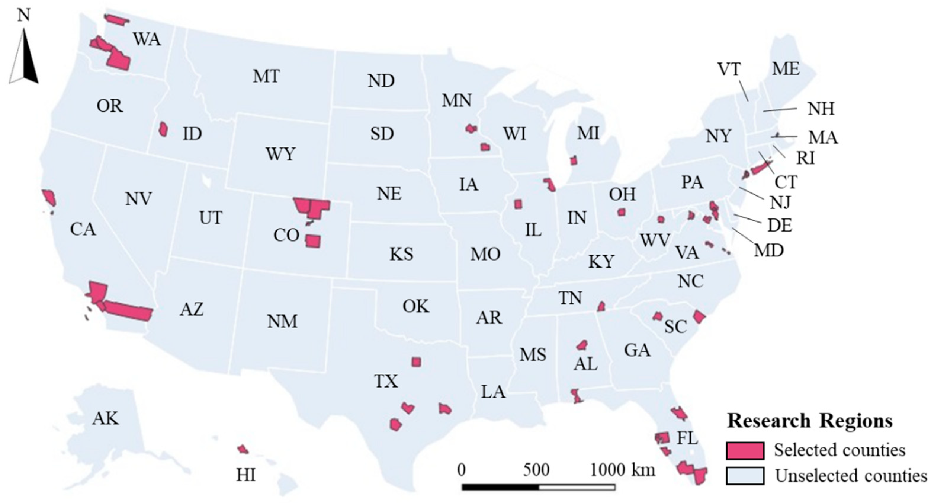
2.2. Dataset
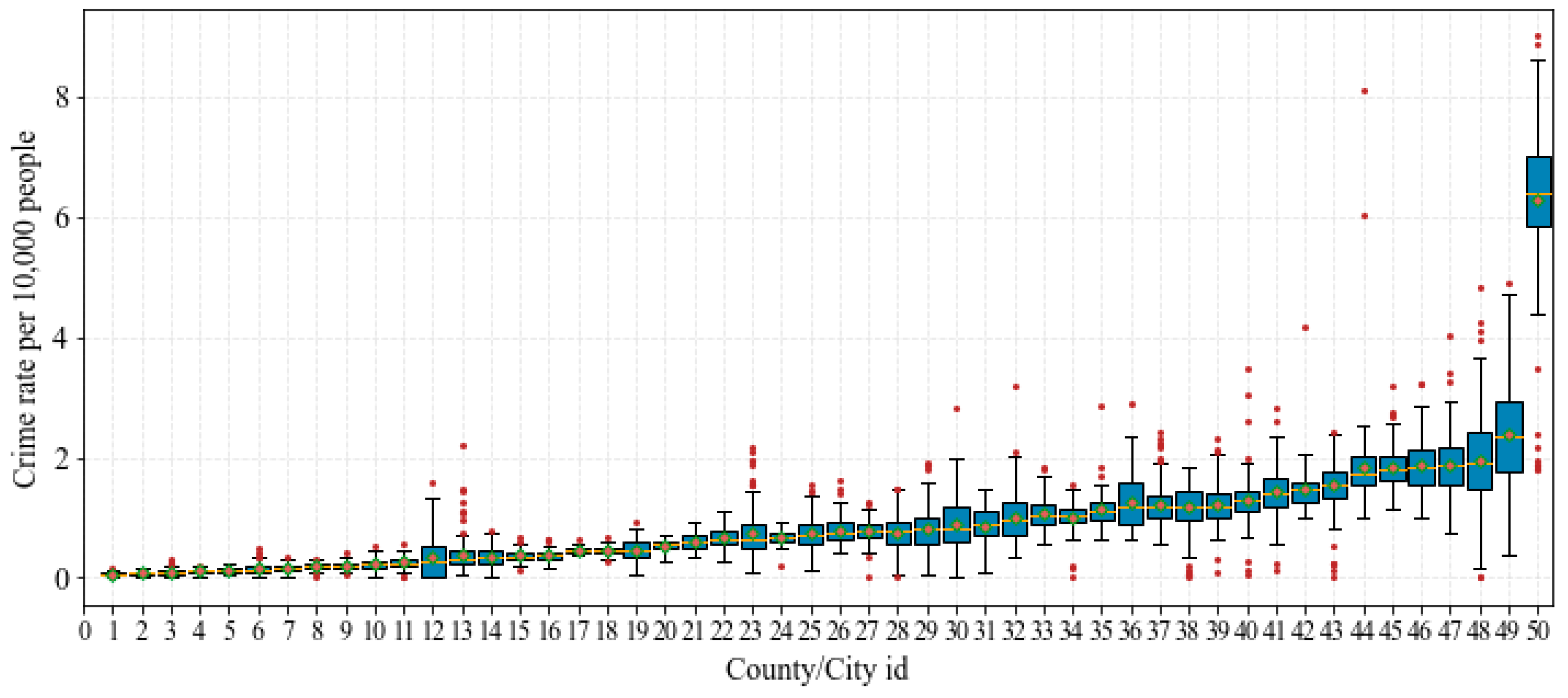
2.2.1. Crime Dataset
- The crime events data missing days for each region should be less than 30 days in 2020 to maintain data consistency for long period time-series analysis.
- The average number of all crime events is higher than 15 each day in individual regions to avoid data noising by small samples.
2.2.2. Driving Factors Datasets
2.3. Methods
2.3.1. Spatial Distribution Analysis
2.3.2. Logistic Regression Model
- (1)
- Dependent variable definition
- (2)
- Independent variables selection
- (3)
- Modeling building
3. Results
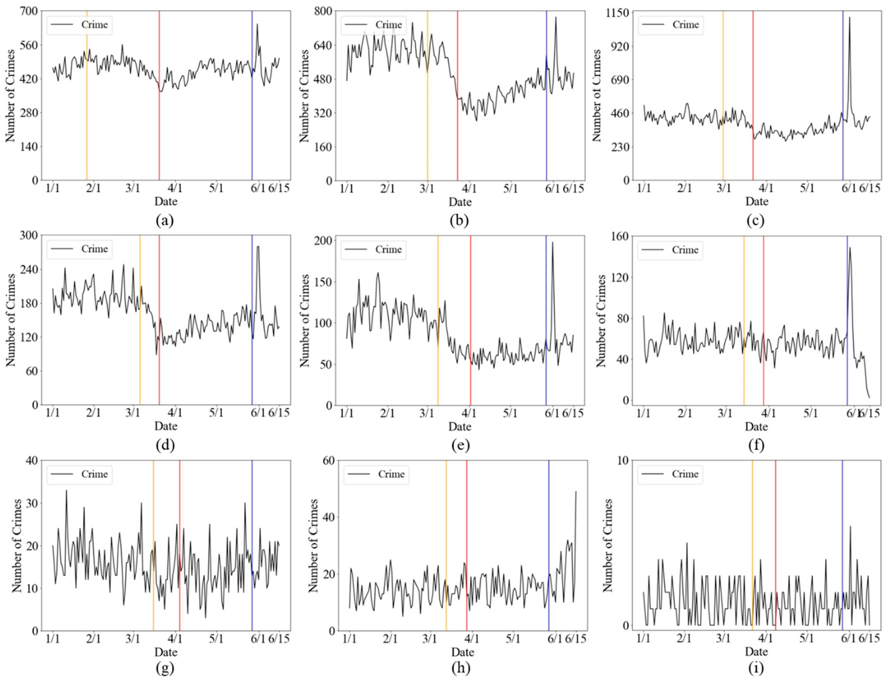
3.1. Overall Trend of Crime during COVID-19 Pandemic
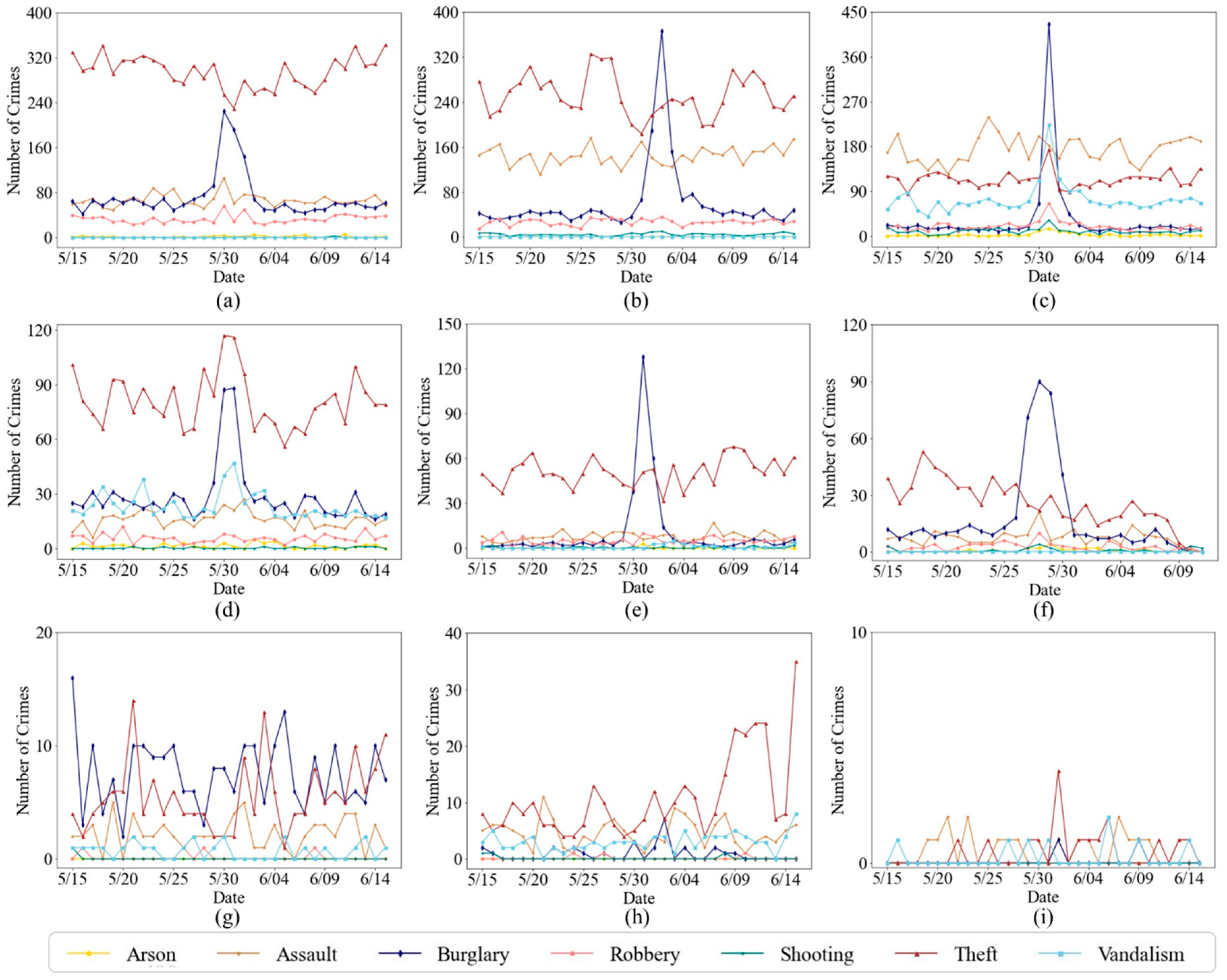
3.2. Changes in Different Crime Types during Black Lives Matter Protests
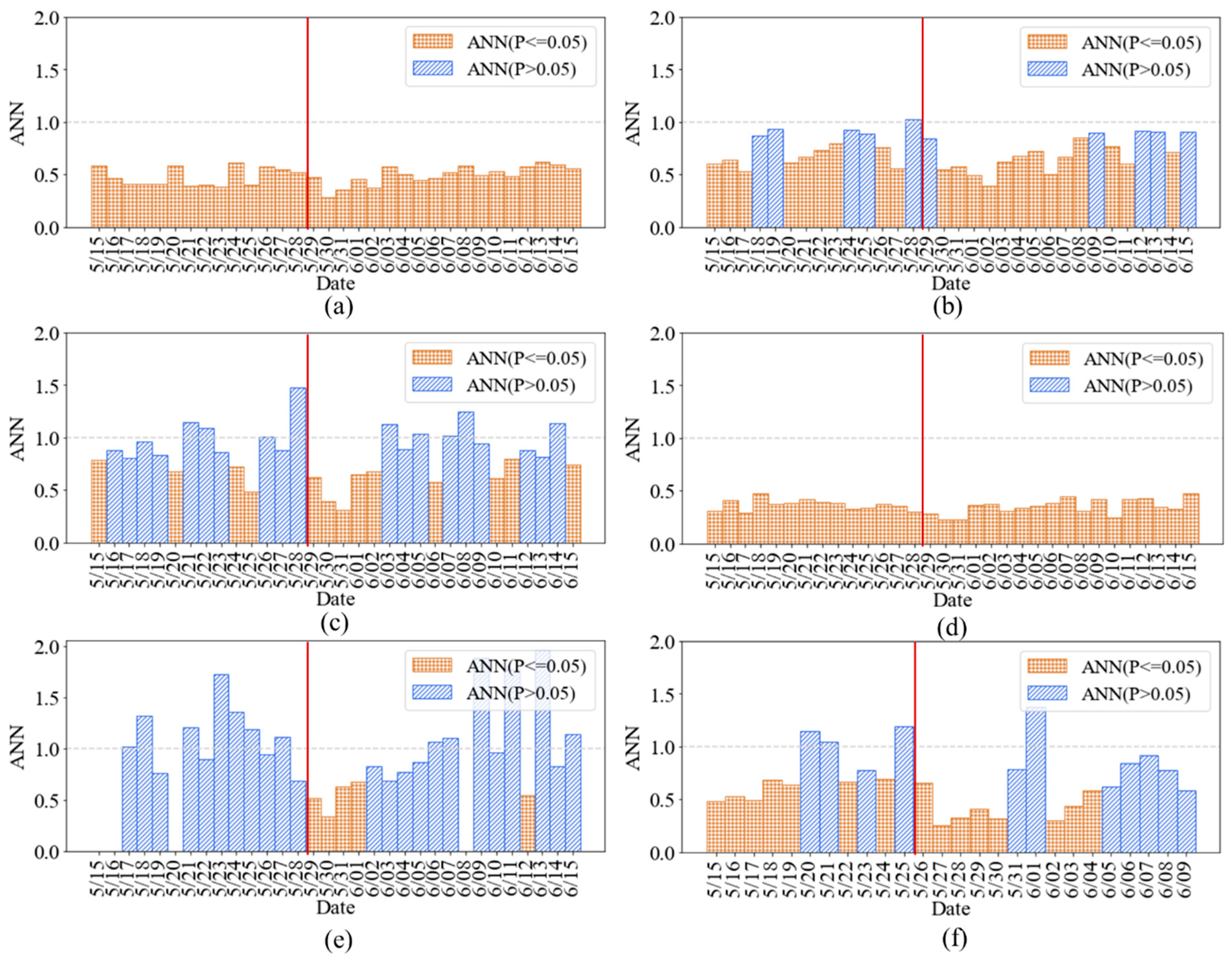
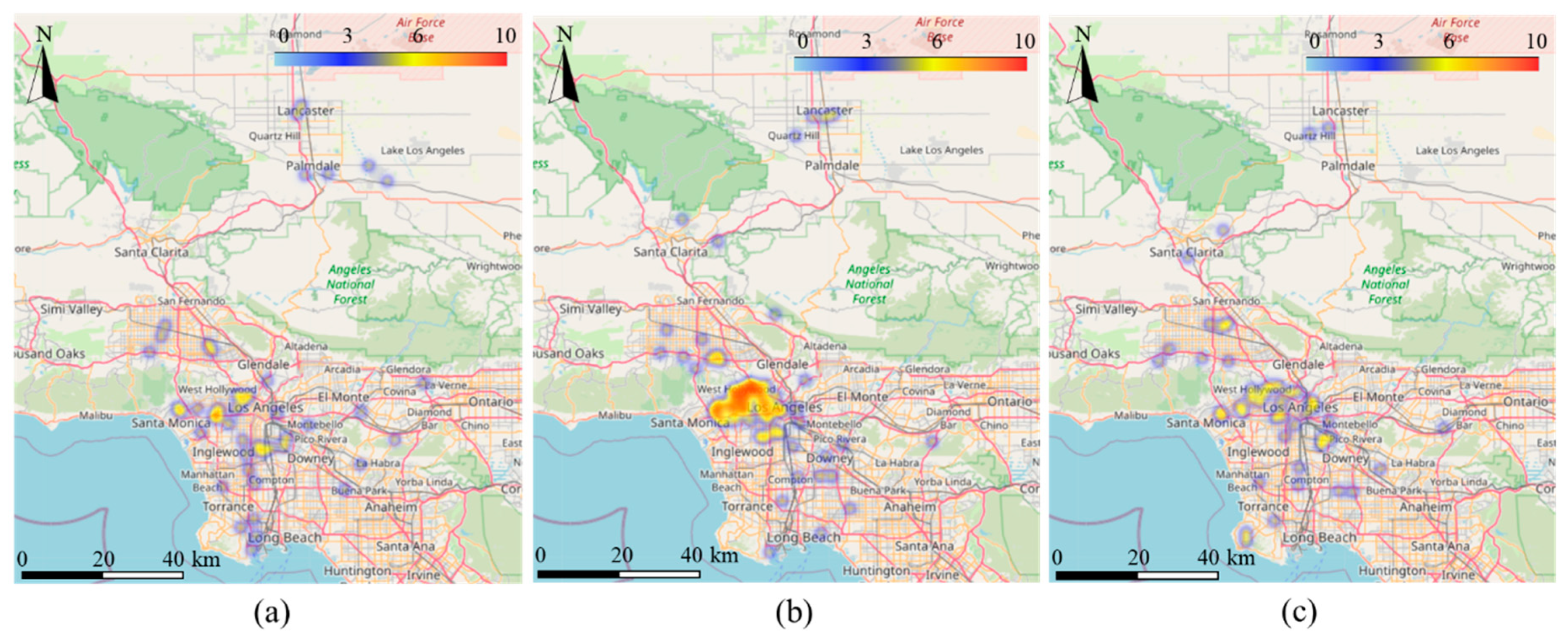
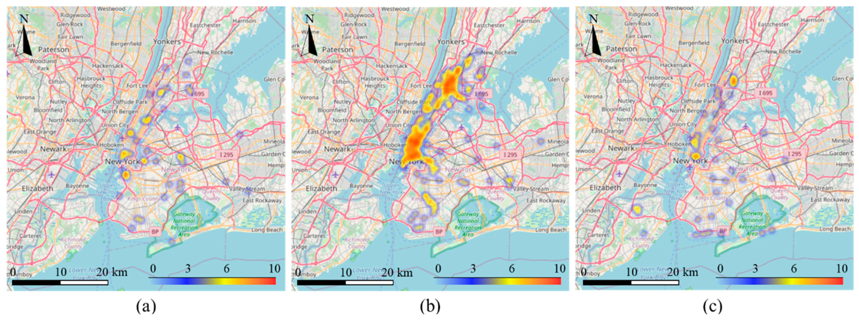
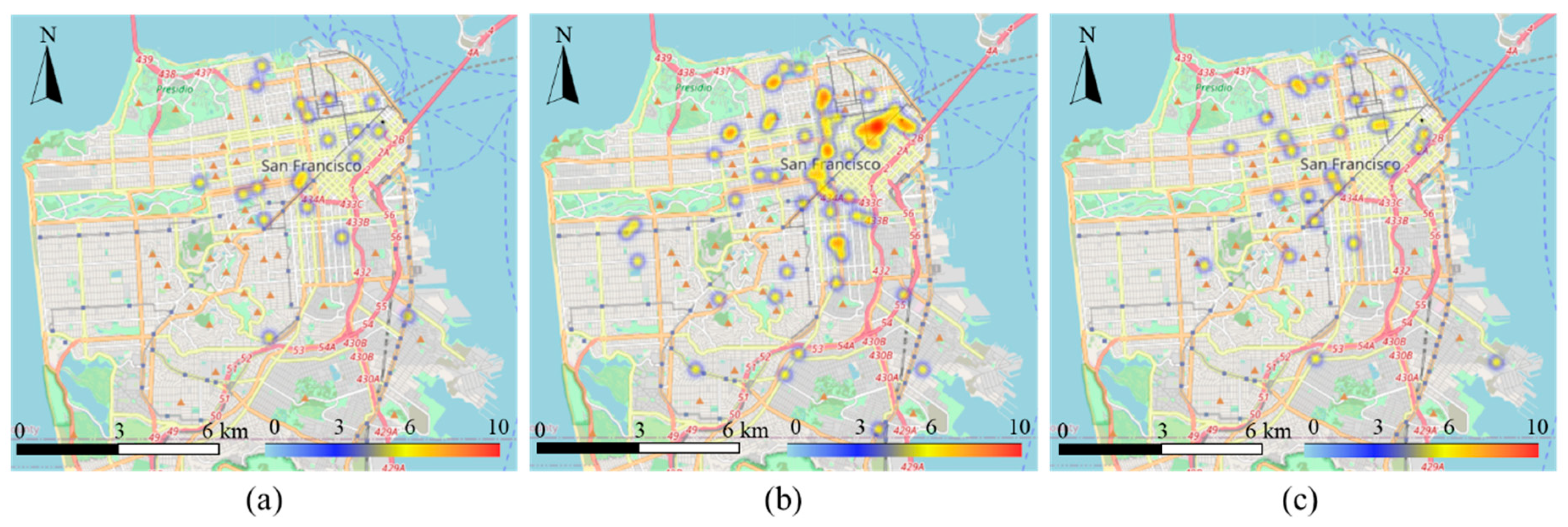
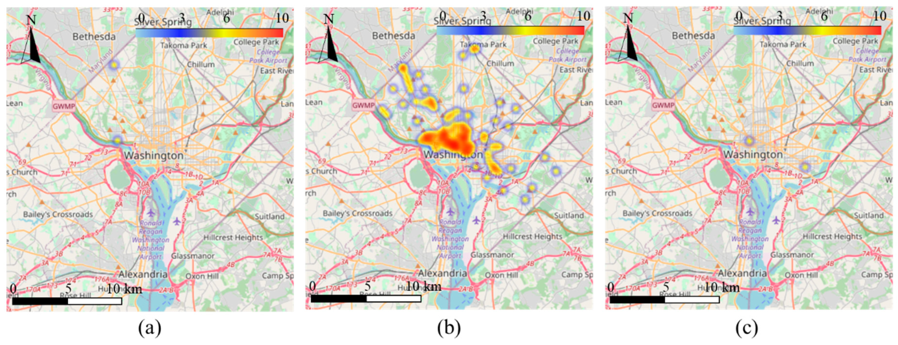
3.3. Spatiotemporal Variations of Burglary during Black Lives Matter Protests
3.4. Impact of Driving Factors on Burglary during Black Lives Matter Protests
3.4.1. Changing Rate of Burglary
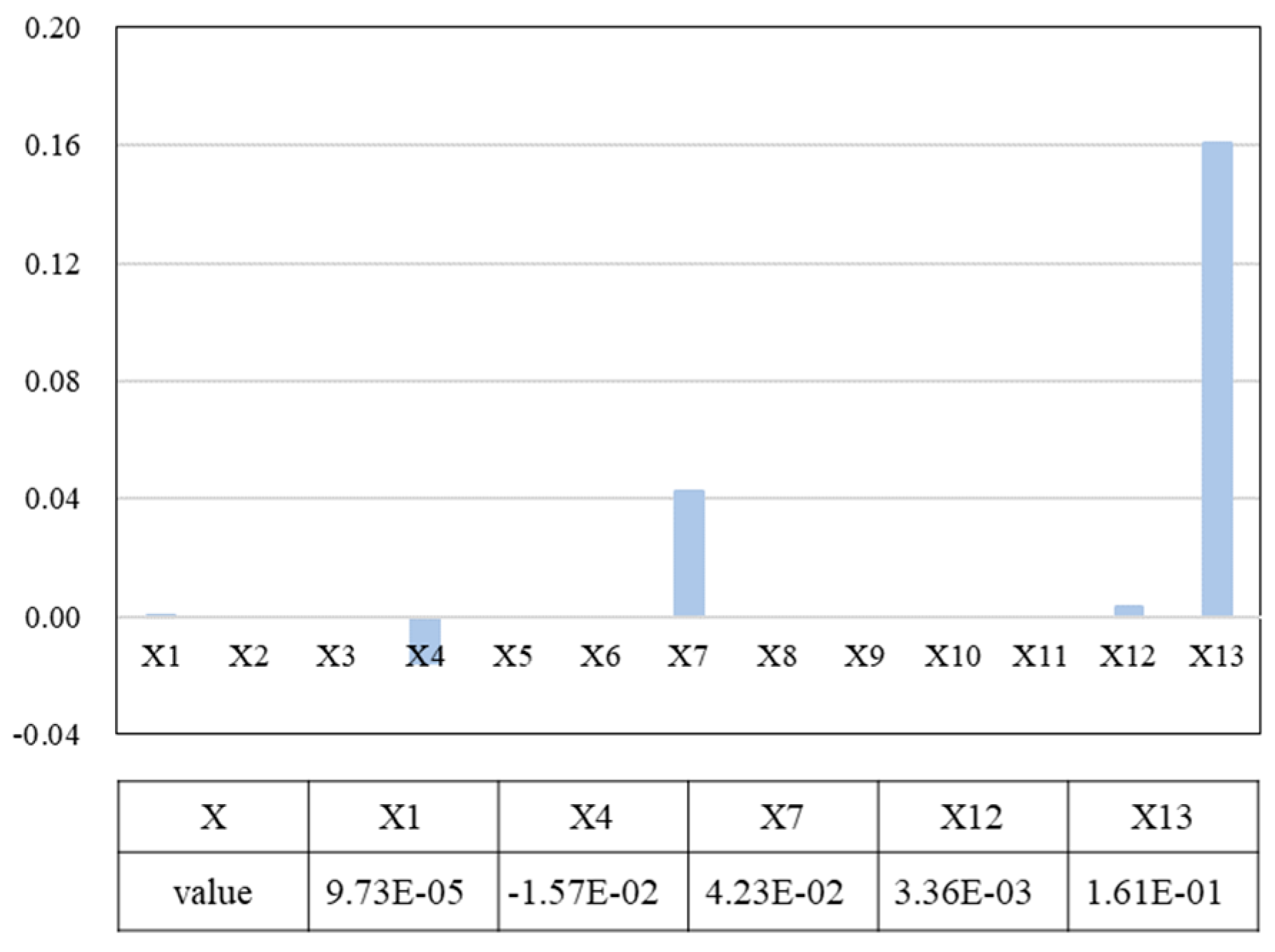
3.4.2. Independent Variables Selection
3.4.3. Driving Factors Analysis
4. Discussion
5. Conclusions
Author Contributions
Funding
Acknowledgments
Conflicts of Interest
References
- Roth, R.E.; Ross, K.S.; Finch, B.G.; Luo, W.; Maceachren, A.M. Spatiotemporal crime analysis in U.S. law enforcement agencies: Current practices and unmet needs. Gov. Inf. Q. 2013, 30, 226–240. [Google Scholar] [CrossRef]
- Duan, L.; Hu, T.; Cheng, E.; Zhu, J.; Gao, C. Deep Convolutional Neural Networks for Spatiotemporal Crime Prediction. In Proceedings of the International Conference on Information and Knowledge Engineering (IKE), Las Vegas, NV, USA, 17–20 July 2017. [Google Scholar]
- Smith, W.R.; Frazee, S.G.; Davison, E.L. Furthering the integration of routine activity and social disorganization theories: Small units of analysis and the study of street robbery as a diffusion process. Criminology 2000, 38, 489–524. [Google Scholar] [CrossRef]
- Sampson, R.J.; Groves, W.B. Community structure and crime: Testing social-disorganization theory. Am. J. Sociol. 1989, 94, 774–802. [Google Scholar] [CrossRef] [Green Version]
- Cohen, L.E.; Felson, M. Social change and crime rate trends: A routine activity approach. Am. Sociol. Rev. 1979, 44, 588–608. [Google Scholar] [CrossRef]
- Felson, M. Environmental Criminology and Crime Analysis, 2nd ed.; Routledge: New York, NY, USA, 2008; pp. 87–97. [Google Scholar]
- Andresen, M.A. A spatial analysis of crime in Vancouver, British Columbia: A synthesis of social disorganization and routine activity theory. Can. Geogr. Le Géographe Can. 2006, 50, 487–502. [Google Scholar] [CrossRef]
- Andresen, M.A. Crime measures and the spatial analysis of criminal activity. Br. J. Criminol. 2006, 46, 258–285. [Google Scholar] [CrossRef]
- Eck, J.E.; Guerette, R.T. The Oxford of Handbook of Crime Prevention; Oxford University Press: New York, NY, USA, 2012; pp. 354–383. [Google Scholar]
- Friedersdorf, C. How to Distinguish Between Antifa, White Supremacists, and Black Lives Matter. The Atlantic. Available online: https://www.theatlantic.com/politics/archive/2017/08/drawing-distinctions-antifathe-alt-right-and-black-lives-matter/538320 (accessed on 2 September 2020).
- Taylor, D.B. George Floyd Protests: A Timeline. New York Times, 10 July 2020. [Google Scholar]
- Dave, D.M.; Friedson, A.I.; Matsuzawa, K.; Sabia, J.J.; Safford, S. Black Lives Matter Protests, Social Distancing, and COVID-19; 0898–2937; National Bureau of Economic Research: Cambridge, MA, USA, 2020. [Google Scholar]
- Mohler, G.; Bertozzi, A.L.; Carter, J.; Short, M.B.; Sledge, D.; Tita, G.E.; Uchida, C.D.; Brantingham, P.J. Impact of social distancing during COVID-19 pandemic on crime in Los Angeles and Indianapolis. J. Crim. Justice 2020, 68, 101692. [Google Scholar] [CrossRef]
- Yang, C.; Sha, D.; Liu, Q.; Li, Y.; Lan, H.; Guan, W.W.; Hu, T.; Li, Z.; Zhang, Z.; Thompson, J.H. Taking the pulse of COVID-19: A spatiotemporal perspective. Int. J. Digit. Earth 2020, 10, 1186–1211. [Google Scholar] [CrossRef]
- Hu, T.; Guan, W.; Zhu, X.; Shao, Y.; Liu, L.; Du, J.; Liu, H.; Zhou, H.; Wang, J.; She, B.; et al. Building an Open Resources Repository for COVID-19 Research. Data Inf. Manag. 2020, 4, 130–147. [Google Scholar]
- Sha, D.; Miao, X.; Lan, H.; Stewart, K.; Ruan, S.; Tian, Y.; Yang, C. Spatiotemporal analysis of medical resource deficiencies in the U.S. under COVID-19 pandemic. PLoS ONE 2020, 15, 1–23. [Google Scholar] [CrossRef]
- Payne, J.; Morgan, A. COVID-19 and Violent Crime: A Comparison of Recorded Offence Rates and Dynamic Forecasts (ARIMA) for March 2020 in Queensland, Australia. SocArXiv de9nc, Center for Open Science. 2020. Available online: https://ideas.repec.org/p/osf/socarx/g4kh7.html (accessed on 2 September 2020).
- Piquero, A.R.; Riddell, J.R.; Bishopp, S.A.; Narvey, C.; Reid, J.A.; Piquero, N.L. Staying Home, Staying Safe? A Short-Term Analysis of COVID-19 on Dallas Domestic Violence. Am. J. Crim. Justice 2020, 3, 1–35. [Google Scholar] [CrossRef] [PubMed]
- Felson, M.; Jiang, S.; Xu, Y. Routine activity effects of the Covid-19 pandemic on burglary in Detroit, March, 2020. Crime Sci. 2020, 9, 10. [Google Scholar] [CrossRef] [PubMed]
- 250 Fined for Breaking 1.5 Metre Rule, but ‘Traditional’ Crime Drops Sharply. Available online: https://www.dutchnews.nl/news/2020/04/250-fined-for-breaking-1-5-metre-rule-but-traditional-crime-drops-sharply/ (accessed on 2 September 2020).
- Rosenfeld, R.; Lopez, E. Pandemic, Social Unrest, and Crime in U.S. Cities: August 2020 Update; Council on Criminal Justice: Washington, WA, USA, 2020. [Google Scholar]
- Pyrooz, D.C.; Decker, S.H.; Wolfe, S.E.; Shjarback, J.A. Was there a Ferguson Effect on crime rates in large U.S. cities? J. Crim. Justice 2016, 46, 1–8. [Google Scholar] [CrossRef]
- Updegrove, A.H.; Cooper, M.N.; Orrick, E.A.; Piquero, A.R. Red states and Black lives: Applying the racial threat hypothesis to the Black Lives Matter movement. Justice Q. 2020, 37, 85–108. [Google Scholar] [CrossRef]
- How Average Nearest Neighbor Works. Available online: https://pro.arcgis.com/en/pro-app/tool-reference/spatial-statistics/h-how-average-nearest-neighbor-distance-spatial-st.htm (accessed on 2 September 2020).
- Silverman, B.W. Density Estimation for Statistics and Data Analysis; CRC Press: Boca Raton, FL, USA, 1986; Volume 26. [Google Scholar]
- SpotCrime. Available online: https://spotcrime.com/ (accessed on 2 September 2020).
- Corso, A.J. Toward predictive crime analysis via social media, big data, and gis spatial correlation. In iConference 2015; iSchools: Newport Beach, CA, USA, 2015. [Google Scholar]
- UCR Offense Definitions. Available online: https://www.ucrdatatool.gov/offenses.cfm (accessed on 2 September 2020).
- Esri. 2020 Esri US Diversity Index Methodology Statement. Available online: https://downloads.esri.com/esri_content_doc/dbl/us/J10170_US_Diversity_Index_2020.pdf (accessed on 2 September 2020).
- Esri. Diversity in the United States. Available online: https://www.arcgis.com/home/item.html?id=def0151deab74cdb881eb92ea6d860d4 (accessed on 2 September 2020).
- Chainey, S.; Tompson, L.; Uhlig, S. The utility of hotspot mapping for predicting spatial patterns of crime. Secur. J. 2008, 21, 4–28. [Google Scholar] [CrossRef]
- Nitta, G.R.; Rao, B.Y.; Sravani, T.; Ramakrishiah, N.; BalaAnand, M. LASSO-based feature selection and naïve Bayes classifier for crime prediction and its type. Serv. Oriented Comput. Appl. 2019, 13, 187–197. [Google Scholar] [CrossRef]
- Santosa, F.; Symes, W.W. Linear inversion of band-limited reflection seismograms. SIAM J. Sci. Stat. Comput. 1986, 7, 1307–1330. [Google Scholar] [CrossRef]
- Tibshirani, R. Regression shrinkage and selection via the lasso. J. R. Stat. Soc. Ser. B 1996, 58, 267–288. [Google Scholar] [CrossRef]
- Fonti, V.; Belitser, E. Feature selection using lasso. VU Amst. Res. Pap. Bus. Anal. 2017, 30, 1–25. [Google Scholar]
- Hosmer, D.W., Jr.; Lemeshow, S.; Sturdivant, R.X. Applied Logistic Regression; John Wiley & Sons: Hoboken, NJ, USA, 2013; Volume 398. [Google Scholar]
- Hoonhout, T. Homicides in Los Angeles Increase 250 Percent from Previous Week. Available online: https://news.yahoo.com/homicides-los-angeles-increase-250-125611007.html (accessed on 2 September 2020).
- McEvoy, J. 14 Days of Protests, 19 Dead. Available online: https://www.forbes.com/sites/jemimamcevoy/2020/06/08/14-days-of-protests-19-dead/#4d7181ca4de4 (accessed on 2 September 2020).
- Rodgers, J.L.; Nicewander, W.A. Thirteen Ways to Look at the Correlation Coefficient. Am. Stat. 1988, 42, 59–66. [Google Scholar] [CrossRef]
- Stigler, S.M. Francis Galton‘s account of the invention of correlation. Stat. Sci. 1989, 4, 73–79. [Google Scholar] [CrossRef]
- Lochner, L. Non-Production Benefits of Education: Crime, Health, and Good Citizenship; CIBC Working Paper, No. 2010-7; The University of Western Ontario, CIBC Centre for Human Capital and Productivity: London, ON, Canada, 2010. [Google Scholar]
- Machin, S.; Marie, O.; Vujić, S. The crime reducing effect of education. Econ. J. 2011, 121, 463–484. [Google Scholar] [CrossRef] [Green Version]
- Parker, K.H.; Juliana, M.; Anderson, M. Amid Protests, Majorities Across Racial and Ethnic Groups Express Support for the Black Lives Matter Movement. Available online: https://tinyurl.com/ycslfon5. (accessed on 2 September 2020).
- Goldberger, S.; Rosenfeld, R. Understanding Crime Trends: Workshop Report; The National Academies Press: Washington, WA, USA, 2008. [Google Scholar]
- Yang, C.; Clarke, K.; Shekhar, S.; Tao, C.V. Big Spatiotemporal Data Analytics: A research and innovation frontier. Int. J. Geogr. Inf. Sci. 2020, 34, 1075–1088. [Google Scholar] [CrossRef] [Green Version]


| ID | County/City Name | ID | County/City Name | ID | County/City Name |
|---|---|---|---|---|---|
| 1 | Tarrant County, TX | 18 | Suffolk County, NY | 35 | Boston, MA |
| 2 | Franklin County, OH | 19 | Ada County, ID | 36 | Washington, DC |
| 3 | Larimer County, CO | 20 | Miami-Dade County, FL | 37 | Montgomery County, TX |
| 4 | Travis County, TX | 21 | New York, NY | 38 | Baltimore County, MD |
| 5 | Bexar County, TX | 22 | Hamilton County, TN | 39 | Henrico County, VA |
| 6 | Sonoma County, CA | 23 | Skagit County, WA | 40 | Minneapolis, MN |
| 7 | Volusia County, FL | 24 | Riverside County, CA | 41 | Newport News, VA |
| 8 | Orange County, CA | 25 | Shelby County, AL | 42 | Chicago, IL |
| 9 | Pierce County, WA | 26 | Fairfax County, VA | 43 | Horry County, SC |
| 10 | Weld County, CO | 27 | Thurston County, WA | 44 | St. Paul, MN |
| 11 | El Paso County, CO | 28 | Collier County, FL | 45 | Denver, CO |
| 12 | Newberry County, SC | 29 | Ottawa County, MI | 46 | San Francisco, CA |
| 13 | Yakima County, WA | 30 | Frederick County, VA | 47 | Norfolk, VA |
| 14 | Sarasota County, FL | 31 | Anne Arundel County, MD | 48 | Harrison County, WV |
| 15 | Pinellas County, FL | 32 | Olmsted County, MN | 49 | Knox County, IL |
| 16 | Hillsborough County, FL | 33 | Escambia County, FL | 50 | Baltimore, MD |
| 17 | Los Angeles County, CA | 34 | Honolulu, HI |
| Category | Factors | Minimum | Mean | Median | Maximum | Standard Deviation |
|---|---|---|---|---|---|---|
| demographic | Population density | 57.83 | 2671.15 | 796.24 | 27,903.88 | 4787.42 |
| Population under 18 years, % | 13.44 | 21.88 | 22.19 | 29.85 | 3.09 | |
| Population over 60 years, % | 13.97 | 21.53 | 19.72 | 43.46 | 5.56 | |
| Age dependency ratio, % | 39.80 | 60.41 | 60.25 | 99.80 | 10.81 | |
| Males per 100 females, % | 88.60 | 96.75 | 97.05 | 109.40 | 3.94 | |
| education | Less than 9th grade, % | 1.30 | 4.94 | 4.25 | 15.60 | 2.88 |
| Bachelor’s degree, % | 16.00 | 34.98 | 34.70 | 61.10 | 10.01 | |
| economic | Median household income, $ | 42,765.00 | 66,186.66 | 64,416.50 | 12,1133.00 | 15,779.62 |
| poverty | Below poverty level, % | 14.90 | 23.97 | 23.20 | 33.30 | 4.29 |
| race | White, % | 21.59 | 73.10 | 79.32 | 95.49 | 17.11 |
| Black or African American, % | 1.12 | 14.59 | 9.36 | 62.73 | 13.38 | |
| Diversity index | 13.00 | 60.42 | 61.50 | 87.00 | 15.83 | |
| crime | 2019 crime rate per 10,000 | 0.04 | 0.98 | 0.76 | 6.09 | 0.97 |
| County/City Name | Class | County/City Name | Class | ||||||
|---|---|---|---|---|---|---|---|---|---|
| Collier County, FL | 7.60 | 4.60 | −39.47 | 0 | Pinellas County, FL | 12.60 | 16.00 | 26.98 | 0 |
| Baltimore County, MD | 10.20 | 6.60 | −35.29 | 0 | Shelby County, AL | 6.20 | 8.20 | 32.26 | 0 |
| Honolulu, HI | 8.20 | 5.80 | −29.27 | 0 | Sarasota County, FL | 3.40 | 5.00 | 47.06 | 0 |
| Miami-Dade County, FL | 9.00 | 7.80 | −13.33 | 0 | Denver, CO | 13.40 | 21.60 | 61.19 | 1 |
| Montgomery County, TX | 6.00 | 5.80 | −3.33 | 0 | Baltimore, MD | 43.80 | 70.80 | 61.64 | 1 |
| Orange County, CA | 23.20 | 23.20 | 0.00 | 0 | Hillsborough County, FL | 8.60 | 18.60 | 116.28 | 1 |
| Pierce County, WA | 2.80 | 2.80 | 0.00 | 0 | Los Angeles County, CA | 64.00 | 144.40 | 125.63 | 1 |
| Riverside County, CA | 15.40 | 15.60 | 1.30 | 0 | San Francisco, CA | 23.00 | 54.60 | 137.39 | 1 |
| Thurston County, WA | 5.80 | 6.00 | 3.45 | 0 | New York, NY | 38.20 | 136.60 | 257.59 | 1 |
| Bexar County, TX | 4.40 | 4.60 | 4.55 | 0 | Minneapolis, MN | 13.00 | 59.00 | 353.85 | 1 |
| Suffolk County, NY | 3.80 | 4.20 | 10.53 | 0 | Fairfax County, VA | 1.40 | 7.60 | 442.86 | 1 |
| Escambia County, FL | 6.80 | 7.60 | 11.76 | 0 | Boston, MA | 2.60 | 19.80 | 661.54 | 1 |
| Hamilton County, TN | 6.20 | 7.00 | 12.90 | 0 | Chicago, IL | 13.00 | 129.40 | 895.38 | 1 |
| Knox County, IL | 4.60 | 5.40 | 17.39 | 0 | St. Paul, MN | 6.40 | 64.40 | 906.25 | 1 |
| Weld County, CO | 2.40 | 3.00 | 25.00 | 0 | Washington, DC | 3.00 | 49.20 | 1540.00 | 1 |
| X1 | X2 | X3 | X4 | X5 | X6 | X7 | X8 | X9 | X10 | X11 | X12 | X13 | |
|---|---|---|---|---|---|---|---|---|---|---|---|---|---|
| X1 | 1.00 | ||||||||||||
| X2 | 0.05 | 1.00 | |||||||||||
| X3 | 0.13 | 0.04 | 1.00 | ||||||||||
| X4 | 0.02 | 0.46 ** | 0.86 ** | 1.00 | |||||||||
| X5 | –0.01 | 0.66 ** | 0.32 * | 0.49 ** | 1.00 | ||||||||
| X6 | 0.44 ** | 0.34 * | 0.11 | 0.22 | 0.17 | 1.00 | |||||||
| X7 | 0.39 ** | 0.17 | 0.08 | 0.01 | 0.34 ** | 0.09 | 1.00 | ||||||
| X8 | 0.30 * | 0.38 ** | 0.18 | 0.22 | 0.46 ** | 0.21 | 0.79 ** | 1.00 | |||||
| X9 | 0.12 | 0.49 ** | 0.31 * | 0.40 ** | 0.55 ** | 0.40 ** | –0.16 | –0.11 | 1.00 | ||||
| X10 | –0.19 | 0.43 ** | 0.46 ** | 0.59 ** | 0.44 ** | 0.16 | 0.03 | 0.24 | 0.32 * | 1.00 | |||
| X11 | 0.48 ** | 0.08 | 0.10 | 0.01 | 0.00 | 0.13 | 0.24 | 0.08 | 0.18 | –0.40 ** | 1.00 | ||
| X12 | 0.42 ** | 0.44 ** | –0.06 | 0.07 | 0.39 ** | 0.69 ** | 0.37 ** | 0.42 ** | 0.27 * | 0.15 | 0.22 | 1.00 | |
| X13 | 0.50 ** | 0.05 | 0.27 * | 0.13 | 0.05 | 0.21 | 0.23 | 0.17 | 0.22 | –0.02 | 0.48 ** | 0.09 | 1.00 |
| Variable | Coefficient | Standard Error | z | P > |z| | Odds Ratios |
|---|---|---|---|---|---|
| Const | –12.666 | 10.136 | –1.250 | 0.211 | 0.000 |
| Population density | 0.000 | 0.000 | 0.753 | 0.451 | 1.000 |
| Age dependency ratio | –0.070 | 0.098 | –0.716 | 0.474 | 0.933 |
| Bachelor’s degree | 0.159 | 0.082 | 1.938 | 0.053 | 1.172 |
| Diversity index | 0.113 | 0.072 | 1.570 | 0.117 | 1.119 |
| 2019 crime rate per 10,000 people | 1.501 | 1.068 | 1.405 | 0.160 | 4.485 |
Publisher’s Note: MDPI stays neutral with regard to jurisdictional claims in published maps and institutional affiliations. |
© 2020 by the authors. Licensee MDPI, Basel, Switzerland. This article is an open access article distributed under the terms and conditions of the Creative Commons Attribution (CC BY) license (http://creativecommons.org/licenses/by/4.0/).
Share and Cite
Zhang, Z.; Sha, D.; Dong, B.; Ruan, S.; Qiu, A.; Li, Y.; Liu, J.; Yang, C. Spatiotemporal Patterns and Driving Factors on Crime Changing During Black Lives Matter Protests. ISPRS Int. J. Geo-Inf. 2020, 9, 640. https://0-doi-org.brum.beds.ac.uk/10.3390/ijgi9110640
Zhang Z, Sha D, Dong B, Ruan S, Qiu A, Li Y, Liu J, Yang C. Spatiotemporal Patterns and Driving Factors on Crime Changing During Black Lives Matter Protests. ISPRS International Journal of Geo-Information. 2020; 9(11):640. https://0-doi-org.brum.beds.ac.uk/10.3390/ijgi9110640
Chicago/Turabian StyleZhang, Zhiran, Dexuan Sha, Beidi Dong, Shiyang Ruan, Agen Qiu, Yun Li, Jiping Liu, and Chaowei Yang. 2020. "Spatiotemporal Patterns and Driving Factors on Crime Changing During Black Lives Matter Protests" ISPRS International Journal of Geo-Information 9, no. 11: 640. https://0-doi-org.brum.beds.ac.uk/10.3390/ijgi9110640